Convergence Rate of the Modified Landweber Method for Solving Inverse Potential Problems

Abstract

In this paper, we present the convergence rate analysis of the modified Landweber method under logarithmic source condition for nonlinear ill-posed problems. The regularization parameter is chosen according to the discrepancy principle. The reconstructions of the shape of an unknown domain for an inverse potential problem by using the modified Landweber method are exhibited.

1. Introduction

An inverse potential problem consists in determining the shape of an unknown domain D form measurements of the Neumann boundary values of u on $\partial \Omega$, where the solution u of the homogeneous Dirichlet problem fulfills

$$\begin{array}{cc}\hfill \Delta u={\chi }_D& \mathrm{in} {\Omega }_R\backslash \partial D,\hfill \end{array}$$

(1)

$$\begin{array}{cc}\hfill u=0& \mathrm{on} \partial {\Omega }_R\hfill \end{array}$$

(2)

where ${\chi }_D$ is the characteristic function of the domain $D\subset {\Omega }_R=\{x\in {\mathbb{R}}^2:\left|x\right|<R\}$. This inverse problem is a nonlinear severely ill-posed problem; see [1,2]. If a classical difference method is used for solving the inverse problem, the errors can grow exponentially fast as the mesh size goes to zero. Many regularizing methods are adopted to provide a stable solution of inverse potential problems, e.g., a second-degree method with frozen derivatives [3], level set regularization [4], the iteratively regularized Gauss–Newton method [5] and Levenberg–Marquardt method [1]. In this work, we consider a discrete version analoguous to the modified asymptotic regularization proposed by Pornsawad et al. [6] to recover the starlike shape of the unknown domain D.

In a general setting, an inverse potential problem can be formulated via a nonlinear operator equation

$$\begin{array}{c}\hfill F\left(x\right)=y,\end{array}$$

(3)

where y is the normal derivative of u on the boundary, $\frac{\partial u}{\partial \nu }{|}_{\partial {\Omega }_R}$, $\nu$ is the outer normal vector on $\partial {\Omega }_R$, the operator $F:\mathcal{D}\left(F\right)\subseteq X\to Y$ is a nonlinear operator on domain $\mathcal{D}\left(F\right)\subset X$, X and Y are Hilbert spaces, and the unknown x includes the information of the domain $D\subset {\Omega }_R$. For convenience in this article, the indices of inner products $⟨·,·⟩$ and norms $\parallel ·\parallel$ are neglected but they can always be identified from the context in which they appear. Due to the nonlinearity of Equation (3), we assume all over that Equation (3) has a solution $x^{+}$ which needs not to be unique. We have the disturbed data $y^{\delta }$ with

$$\begin{array}{c}\hfill ∥y^{\delta }-y∥\le \delta \end{array}$$

(4)

where $\delta >0$ is a noise level. If one solves Equation (3) by traditional numerical method, high oscillating solutions may occur. Thus, one needs a regularization to minimize the approximation and data error.

One well-known continuous regularization is Showalter’s method or asymptotic regularization [7], where an approximate solution is obtained by solving an initial value problem. Later, a second-order asymptotic regularization for the linear problem $Ax=y$ was investigated in Zhang and Hofmann [8], where the optimal order is obtained under the Hölder type source condition and a conventional discrepancy principle as well as a total energy discrepancy principle. Recently, the study of modified asymptotic regularization is reported in Pornsawad et al. [6] where the term $\overline{x}-x^{\delta }\left(t\right),x^{\delta }\left(0\right)=\overline{x},$ is included to the method proposed by Tautenhahn [7], i.e.,

$$\begin{array}{c}\hfill {\dot{x}}^{\delta }\left(t\right)=F^{\prime }{\left(x^{\delta }\left(t\right)\right)}^{*}[y^{\delta }-F\left(x^{\delta }\left(t\right)\right)]-(x^{\delta }\left(t\right)-\overline{x}),0<t\le T.\end{array}$$

(5)

A discrete version analogue to Equation (5) is successfully developed in Pornsawad and Böckmann [9], where the whole family of Runge–Kutta methods is applied and one obtaines an optimal convergence rate under Hölder-type sourcewise condition if the Fréchet derivative is properly scaled and locally Lipschitz continuous.

It is well known that, for many applications such as the inverse potential problem and the inverse scattering problem [5], the Hölder type source condition in general is not fulfilled even if a solution is very smooth. It is applicable only for mildly ill-posed problems [1,10,11]. Therefore, the convergence rate analysis of an explicit Euler method presented by

$$\begin{array}{c}\hfill x_{n+1}^{\delta }=x_n^{\delta }+F^{\prime }{\left(x_n^{\delta }\right)}^{*}(y^{\delta }-F\left(x_n^{\delta }\right))-{\alpha }_n(x_n^{\delta }-x_0)\end{array}$$

(6)

is considered in this article under the logarithmic source condition in Equation (7) and the properly scaled Fréchet derivative $\parallel F^{\prime }\left(x^{+}\right)\parallel \le 1$. The method in Equation (6) is a particular method of the iterative Runge–Kutta-type method [9], where ${\tau }_n={\alpha }_n^{-1}$ is the relaxation parameter obtained by discretization of conventional asymptotic regularization [7]. We define

$$f=f_p,f_p\left(\lambda \right):=\left\{\begin{array}{cc}{\left(ln\frac{\mathrm{e}}{\lambda }\right)}^{-p}\hfill & \mathrm{for}0<\lambda \le 1\hfill \\ 0\hfill & \mathrm{for}\lambda =0\hfill \end{array}\right.$$

(7)

with $p>0$ and the usual sourcewise representation

$$\begin{array}{c}\hfill x^{+}-x_0=f\left(F^{\prime }{\left(x^{+}\right)}^{*}{F}^{\prime }\left(x^{+}\right)\right)w,w\in X\end{array}$$

(8)

where $∥w∥$ is sufficiently small. The method in Equation (6) is also known as the modified Landweber method [12] which has the rate $O\left(\sqrt{\delta }\right)$ under the Hölder-type source condition and general discrepancy principle. The convergence rate analysis under the logarithmic source condition in Equation (7) has been successfully studied by Hohage [5] for the iteratively regularized Gauss–Newton method and by Deuflhard et al. [13] for Landweber’s iteration. Current studies of source condition may be found, e.g., in Romanov et al. [11], Bakushinsky et al. [14], Schuster et al. [15] and Albani et al. [16].

The purpose of this work is to present the convergence rate analysis of the iterative scheme of Equation (6) under the logarithmic source condition in Equation (7) with $1\le p\le 2$ and to recover the shape of an unknown domain D for an inverse potential problem (Equations (1) and (2)). Thus, in Section 2, a preliminary result is prepared. As usual, the Fréchet derivative of F needs to be scaled. Furthermore, we assume a nonlinearity condition of F in a ball $B_{\rho }\left(x_0\right)=\{x\in X:\parallel x-x_0\parallel \le \rho \},\rho >0$, which is given in Assumption 1. It is well known that, without the additional assumption on the nonlinear operator, the convergence rate cannot be provided. The following assumption has been used in many works [5,17], i.e., there exists a bounded linear operator $R:Y\to Y$ and $Q:X\to Y$ such that

$$\begin{array}{cc}\hfill F^{\prime }\left(\tilde{x}\right)& =R(\tilde{x},x)F^{\prime }\left(x\right)+Q(\tilde{x},x)\hfill \\ \hfill \parallel I-R(\tilde{x},x)\parallel & \le C_R\hfill \\ \hfill \parallel Q(\tilde{x},x)\parallel & \le C_Q\parallel F^{\prime }\left(x^{†}\right)(\tilde{x}-x)\parallel \hfill \end{array}$$

with nonnegative constants $C_R$ and $C_Q$. However a weaker condition will be used in this work. This will be shown in Assumption 1. In Section 3, the convergence rate of the modified Landweber method under the logarithmic source condition is presented. Application of the modified Landweber method to an inverse potential problem is provided in Section 4.

2. Preliminary Results

In this section, preliminary results are prepared to provide the convergence analysis of the modified Landweber method.

Lemma 1.

Let A be a linear operator with $\parallel A\parallel \le 1$. For $n\in N$ with $n>1,e_0:=f\left(\lambda \right)w$ with f given by Equation (7) and $p>0$, there exist positive constants $c_1$ and $c_2$ such that

$$\begin{array}{c}\hfill ∥\prod _{i=0}^{n-1}(1-{\alpha }_i){(I-A^{*}A)}^n{e}_0∥\le c_1{(ln(n+\mathrm{e}))}^{-p}\parallel w\parallel \end{array}$$

(9)

and

$$\begin{array}{c}\hfill ∥A\prod _{i=0}^{n-1}(1-{\alpha }_i){(I-A^{*}A)}^n{e}_0∥\le c_2{(n+1)}^{-1/2}{(ln(n+\mathrm{e}))}^{-p}\parallel w\parallel \end{array}$$

(10)

with $0<{\alpha }_i\le 1,i=0,1,2,\dots ,n.$

Proof. 

By spectral theory and Equations (7), (A1), and (A2), we have

$$\begin{array}{ccc}\hfill ∥\prod _{i=0}^{n-1}(1-{\alpha }_i){(I-A^{*}A)}^n{e}_0∥& \le & \prod _{i=0}^{n-1}(1-{\alpha }_i)\parallel {(I-A^{*}A)}^{n}f\left(A^{*}A\right)\parallel \parallel w\parallel \hfill \\ & \le & \underset{\lambda \in (0,1]}{sup}{|(1-\lambda )}^n{(1-ln\lambda )}^{-p}|\parallel w\parallel \hfill \\ & \le & c_1{(ln(n+\mathrm{e}))}^{-p}\parallel w\parallel \hfill \end{array}$$

(11)

for some constant $c_1>0$. Similary, spectral theory and Equations (7), (A3), and (A4) provides

$$\begin{array}{ccc}\hfill ∥A\prod _{i=0}^{n-1}(1-{\alpha }_i){(I-A^{*}A)}^n{e}_0∥& \le & \prod _{i=0}^{n-1}(1-{\alpha }_i)\parallel {(I-A^{*}A)}^n{\left(A^{*}A\right)}^{1/2}f\left(A^{*}A\right)\parallel \parallel w\parallel \hfill \\ & \le & \underset{\lambda \in (0,1]}{sup}{|(1-\lambda )}^n{\lambda }^{1/2}{(1-ln\lambda )}^{-p}|\parallel w\parallel \hfill \\ & \le & c_2{(n+1)}^{-1/2}{(ln(n+\mathrm{e}))}^{-p}\parallel w\parallel \hfill \end{array}$$

(12)

for some constant $c_2>0$.  □

Proposition 1.

Let A be a linear operator with $\parallel A\parallel \le 1$. For $n\in N$ with $n>1,e_0:=f\left(\lambda \right)w$ with f given by Equation (7) and $p=2\psi$, for some $\psi \in [1/2,1]$, there exist positive constants ${\tilde{c}}_1$ and ${\tilde{c}}_2$ such that

$$∥\sum _{j=0}^{n-1}{\alpha }_{n-j-1}{(I-A^{*}A)}^j\prod _{i=1}^j(1-{\alpha }_{n-i})e_0∥\le {\tilde{c}}_1{(ln(n+\mathrm{e}))}^{-p}\parallel w\parallel$$

(13)

and

$$\parallel A\sum _{j=0}^{n-1}{\alpha }_{n-j-1}{(I-A^{*}A)}^j\prod _{i=1}^j(1-{\alpha }_{n-i})e_0\parallel \le {\tilde{c}}_2{(n+1)}^{-1/2}{(ln(n+\mathrm{e}))}^{-p}\parallel w\parallel$$

(14)

for ${\alpha }_i=\frac{1}{2}{(i+l_0)}^{-\psi },i=0,1,2,\dots ,n$ and $l_0\ge 2$.

Proof. 

We will prove by induction that, for some $c\in \mathbb{R}$, the inequality

$$∥\sum _{j=0}^{k-1}{\alpha }_{n-j-1}{(I-A^{*}A)}^j\prod _{i=1}^j(1-{\alpha }_{n-i})e_0∥\le c{(ln(k+\mathrm{e}))}^{-p}\parallel w\parallel$$

(15)

is true. Note that $\frac{p}{\psi }=2\le \frac{ln2}{ln(ln(1+\mathrm{e}\left)\right)}$ and $l_0\ge 2$ provide

$$\frac{p}{\psi }ln(ln(1+\mathrm{e}))\le ln2\le ln{l}_0\le ln(l_0+n-1).$$

This means that ${(ln(1+\mathrm{e}))}^{-p}\ge {(l_0+n-1)}^{-\psi }.$ Using Equation (7), we have

$$\begin{array}{ccc}\hfill \parallel {\alpha }_{n-1}{(I-A^{*}A)}^0{e}_0\parallel & \le & \frac{1}{2}{(n-1+l_0)}^{-\psi }\underset{\lambda \in (0,1]}{sup}|{(1-ln\lambda )}^{-p}|\parallel w\parallel \hfill \\ & \le & \frac{1}{2}{(ln(1+\mathrm{e}))}^{-p}\parallel w\parallel .\hfill \end{array}$$

Thus, Equation (15) holds for $k=1$. Next, we assume that Equation (15) holds for $k-1<n$ for some constant c. Applying Lemma 1, we obtain

$$\begin{array}{cc}& ∥\sum _{j=0}^k{\alpha }_{n-j-1}{(I-A^{*}A)}^j\prod _{i=1}^j(1-{\alpha }_{n-i})e_0∥\hfill \\ \le & ∥\sum _{j=0}^{k-1}{\alpha }_{n-j-1}{(I-A^{*}A)}^j\prod _{i=1}^j(1-{\alpha }_{n-i})e_0∥+∥{\alpha }_{n-k-1}{(I-A^{*}A)}^k\prod _{i=1}^k(1-{\alpha }_{n-i})e_0∥\hfill \\ \le & c{(ln(k+\mathrm{e}))}^{-p}\parallel w\parallel +\frac{1}{2}{(n-k-1+l_0)}^{-\psi }∥{(I-A^{*}A)}^{k}f\left(A^{*}A\right)w∥\hfill \\ \le & c{(ln(k+\mathrm{e}))}^{-p}\parallel w\parallel +\frac{c_1}{2}{(n-k-1+l_0)}^{-\psi }{(ln(k+\mathrm{e}))}^{-p}\parallel w\parallel .\hfill \end{array}$$

(16)

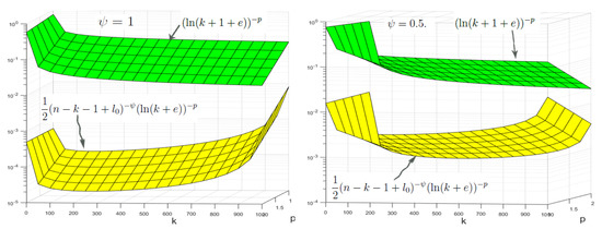
By Figure 1, we observe that

$$\frac{1}{2}{(n-k-1+l_0)}^{-\psi }{(ln(k+\mathrm{e}))}^{-p}\le {(ln(k+1+\mathrm{e}))}^{-p}.$$

Figure 1. Plot of ${(ln(k+1+\mathrm{e}))}^{-p}$ and $\frac{1}{2}{(n-k-1+l_0)}^{-\psi }{(ln(k+\mathrm{e}))}^{-p}$ with $n=1000,l_0=10$, and (left) $\psi =1$ and (right) $\psi =0.5$.

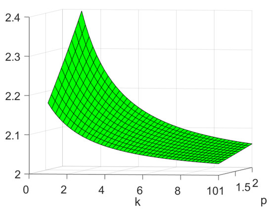
Moreover, in Figure 2, the graph of ${\left(\frac{ln(k+1+\mathrm{e})}{ln(k+\mathrm{e})}\right)}^p+1$ has a maximum at $k=1$ and $p=2$ and the maximum value is ${\left(\frac{ln(2+\mathrm{e})}{ln(1+\mathrm{e})}\right)}^2+1=2.3956$. Thus, Equation (16) becomes

$$\begin{array}{cc}& ∥\sum _{j=0}^k{\alpha }_{n-j-1}{(I-A^{*}A)}^j\prod _{i=1}^j(1-{\alpha }_{n-i})e_0∥\hfill \\ \le & max\{c,c_1\}{(ln(k+1+\mathrm{e}))}^{-p}\parallel w\parallel \left(\frac{{(ln(k+\mathrm{e}))}^{-p}}{{(ln(k+1+\mathrm{e}))}^{-p}}+1\right)\hfill \\ \le & {\tilde{c}}_1{(ln(k+1+\mathrm{e}))}^{-p}\parallel w\parallel \hfill \end{array}$$

for some constant ${\tilde{c}}_1.$ Thus, the induction is complete.

Figure 2. Plot of ${\left(\frac{ln(k+1+\mathrm{e})}{ln(k+\mathrm{e})}\right)}^p+1$.

We prove Equation (14) by induction in the same manner as Equation (13).  □

Assumption 1.

There exist positive constants $c_L$, $c_R$, and $c_r$ and linear bounded operator $R_x:Y\to Y$ such that, for $x\in$$B_{\rho }\left(x_0\right)$, the following condition holds

$$\begin{array}{cc}\hfill F^{\prime }\left(x\right)& =R_x{F}^{\prime }\left(x^{+}\right)\hfill \end{array}$$

(17)

$$\begin{array}{cc}\hfill ∥R_x-I∥& \le c_L∥x-x^{+}∥\hfill \end{array}$$

(18)

$$\begin{array}{cc}\hfill \left|∥R_x∥-∥I∥\right|& \ge c_R\hfill \end{array}$$

(19)

$$\begin{array}{cc}\hfill ∥R_x∥& \le c_r\hfill \end{array}$$

(20)

where $x^{+}$ is the exact solution of Equation (3).

Lemma 2.

Let the Assumption 1 be assumed. Then, we have

$$\begin{array}{c}\hfill ∥(1-{\alpha }_n)I-R_{x_n^{\delta }}^{*}∥\le \frac{1}{2}{K}_R∥e_n∥\end{array}$$

(21)

for some constant $K_R>0$ with $e_n=x^{+}-x_n^{\delta }$.

Proof. 

We note that the reverse triangle inequality and Equation (19) guarantee the estimates

$$\begin{array}{c}\hfill 1\le \frac{∥R_x-I∥}{\left|∥R_x∥-∥I∥\right|}\le c_R^{-1}∥R_x-I∥\end{array}$$

(22)

and

$$\begin{array}{c}\hfill ∥I+R_x^{*}∥\le \frac{1}{\left|∥R_x∥-∥I∥\right|}\times ∥I-R_x^{*}∥∥I+R_x^{*}∥\le c_R^{-1}∥I-R_x^{*}∥∥I+R_x^{*}∥.\end{array}$$

(23)

Using the estimates in Equations (18), (20), (22), and (23) and the triangle inequality, we now have

$$\begin{array}{cc}\hfill ∥(1-{\alpha }_n)I-R_{x_n^{\delta }}^{*}∥& =∥\frac{1}{2}\left[(1-(1+{\alpha }_n))(I+R_{x_n^{\delta }}^{*})\right]+\frac{1}{2}\left[(1+(1-{\alpha }_n))(I-R_{x_n^{\delta }}^{*})\right]∥\hfill \\ \hfill & \le \frac{1}{2}\left[{\alpha }_n{c}_R^{-1}∥I+R_{x_n^{\delta }}^{*}∥+\left|2-{\alpha }_n\right|\right]∥I-R_{x_n^{\delta }}^{*}∥\hfill \\ \hfill & \le \frac{1}{2}{K}_R∥e_n∥\hfill \end{array}$$

with the positive constant $K_R=\left[{\alpha }_n{c}_R^{-1}\left(∥I∥+c_r\right)+\left|2-{\alpha }_n\right|\right]c_L$.  □

Proposition 2.

Let the conditions in Equations (17) and (18) in Assumption 1 be true. Then,

$$\begin{array}{c}\hfill ∥F\left(x_n^{\delta }\right)-F\left(x^{+}\right)-F^{\prime }\left(x^{+}\right)(x_n^{\delta }-x^{+})∥\le \frac{1}{2}{c}_L∥e_n∥∥K{e}_n∥\end{array}$$

(24)

for $x\in$$B_{\rho }\left(x_0\right)$ with $K=F^{\prime }\left(x^{+}\right)$ and $e_n=x^{+}-x_n^{\delta }$.

Proof. 

Define $w_t=x^{+}+t(x_n^{\delta }-x^{+})$ as $0\le t\le 1$. Using the mean value theorem with Equations (17) and (18), we obtain

$$\begin{array}{cc}∥F\left(x_n^{\delta }\right)-F\left(x^{+}\right)-F^{\prime }\left(x^{+}\right)(x_n^{\delta }-x^{+})∥\hfill & =∥{\int }_0^1\left[F^{\prime }(x^{+}+t(x_n^{\delta }-x^{+}))-F^{\prime }\left(x^{+}\right)\right](x_n^{\delta }-x^{+})dt∥\hfill \\ \hfill & \le {\int }_0^1∥R_{w_t}-I∥∥F^{\prime }\left(x^{+}\right)(x_n^{\delta }-x^{+})∥dt\hfill \\ \hfill & \le \frac{1}{2}{c}_L∥e_n∥∥K{e}_n∥.\hfill \end{array}$$

(25)

 □

3. Convergence Analysis

To investigate the convergence rate of the modified Landweber method under the logarithmic source condition, we choose the regularization parameter n according to the generalized discrepancy principle, i.e., the iteration is stopped after N = N($y^{\delta }$,$\delta$) steps with

$$\begin{array}{c}\hfill ∥y^{\delta }-F\left(x_N^{\delta }\right)∥\le \tau \delta <∥y^{\delta }-F\left(x_n^{\delta }\right)∥,0\le n<N\end{array}$$

(26)

where $\tau >\frac{2-\eta }{1-\eta }$ is a positive number. In addition to the discrepancy principle, F satisfies the local property in the open ball $B_{\rho }\left(x_0\right)$ of radius $\rho$ around $x_0$

$$\begin{array}{c}\hfill ∥F\left(x\right)-F\left(\tilde{x}\right)-F^{\prime }\left(x\right)(x-\tilde{x})∥\le \eta ∥F\left(x\right)-F\left(\tilde{x}\right)∥,\eta <\frac{1}{2}\end{array}$$

(27)

with $x,\tilde{x}$∈$B_{\rho }\left(x_0\right)$$\subset \mathcal{D}\left(F\right)$. Utilizing the triangle inequality yields

$$\begin{array}{c}\hfill \frac{1}{1+\eta }∥F^{\prime }\left(x\right)(x-\tilde{x})∥\le ∥F\left(x\right)-F\left(\tilde{x}\right)∥\le \frac{1}{1-\eta }∥F^{\prime }\left(x\right)(x-\tilde{x})∥\end{array}$$

(28)

to ensure at least local convergence to a solution $x^{+}$ of Equation (3) in $B_{\frac{\rho }{2}}\left(x_0\right)$.

Theorem 1.

Assume that the problem in Equation (3) has a solution $x^{+}$ in $B_{\frac{\rho }{2}}\left(x_0\right)$, $y^{\delta }$ fulfills Equation (4), and F satisfies Equations (17) and (18). Assume that the Fréchet derivative of F is scaled such that $∥F^{\prime }\left(x\right)∥\le 1$ for $x\in B_{\frac{\rho }{2}}\left(x_0\right)$. Furthermore, assume that the source condition in Equations (7) and (8) is fulfilled and that the modified Landweber method is stopped according to Equation (26). If $∥w∥$ is sufficiently small, then there exists a constant $K_2$ depending only on p and $∥w∥$ with

$$\begin{array}{c}\hfill ∥e_n∥\le K_2{(lnn)}^{-p}\end{array}$$

(29)

and

$$\begin{array}{c}\hfill ∥y^{\delta }-F\left(x_n^{\delta }\right)∥\le 4K_2{(n+1)}^{-1/2}{(lnn)}^{-p}.\end{array}$$

Proof. 

We give the abbreviation $e_n$:= $x^{+}-x_n^{\delta }$ for the error of the nth iteration $x_n^{\delta }$ of Equation (6) and $K:=F^{\prime }\left(x^{+}\right)$. We can rewrite Equation ( 6) into the form

$$\begin{array}{c}\hfill x^{+}-x_{n+1}^{\delta }=(1-{\alpha }_n)(x^{+}-x_n^{\delta })+F^{\prime }{\left(x_n^{\delta }\right)}^{*}(F\left(x_n^{\delta }\right)-y^{\delta })-{\alpha }_n(x_0-x^{+}).\end{array}$$

Since $e_n$:= $x^{+}-x_n^{\delta }$ and $K:=F^{\prime }\left(x^{+}\right)$, we present $e_n$ as

$$\begin{array}{cc}\hfill e_{n+1}& =(1-{\alpha }_n)e_n+F^{\prime }{\left(x_n^{\delta }\right)}^{*}(F\left(x_n^{\delta }\right)-y^{\delta })-{\alpha }_n(x_0-x^{+})\hfill \\ \hfill & =(1-{\alpha }_n)(I-K^{*}K)e_n+(1-{\alpha }_n)K^{*}K{e}_n+F^{\prime }{\left(x_n^{\delta }\right)}^{*}(F\left(x_n^{\delta }\right)-y^{\delta })-{\alpha }_n(x_0-x^{+})\hfill \\ \hfill & =(1-{\alpha }_n)(I-K^{*}K)e_n+(1-{\alpha }_n)K^{*}\left[F\left(x_n^{\delta }\right)-F\left(x^{+}\right)-K(x_n^{\delta }-x^{+})\right]\hfill \\ \hfill & +\left[K^{*}-F^{\prime }{\left(x_n^{\delta }\right)}^{*}\right]\left(y^{\delta }-F\left(x_n^{\delta }\right)\right)-{\alpha }_n{K}^{*}(y^{\delta }-F\left(x_n^{\delta }\right))+(1-{\alpha }_n)K^{*}(y-y^{\delta })\hfill \\ \hfill & -{\alpha }_n(x_0-x^{+})\hfill \\ \hfill & =(1-{\alpha }_n)(I-K^{*}K)e_n+(1-{\alpha }_n)K^{*}\left[F\left(x_n^{\delta }\right)-F\left(x^{+}\right)-K(x_n^{\delta }-x^{+})\right]\hfill \\ \hfill & +\left[K^{*}-K^{*}{R}_{x_n^{\delta }}^{*}\right]\left(y^{\delta }-F\left(x_n^{\delta }\right)\right)-{\alpha }_n{K}^{*}(y^{\delta }-F\left(x_n^{\delta }\right))+(1-{\alpha }_n)K^{*}(y-y^{\delta })\hfill \\ \hfill & -{\alpha }_n(x_0-x^{+})\hfill \\ \hfill & =(1-{\alpha }_n)(I-K^{*}K)e_n+(1-{\alpha }_n)K^{*}\left[F\left(x_n^{\delta }\right)-F\left(x^{+}\right)-K(x_n^{\delta }-x^{+})\right]\hfill \\ \hfill & +K^{*}\left[(1-{\alpha }_n)I-R_{x_n^{\delta }}^{*}\right]\left(y^{\delta }-F\left(x_n^{\delta }\right)\right)+(1-{\alpha }_n)K^{*}(y-y^{\delta })\hfill \\ \hfill & -{\alpha }_n(x_0-x^{+}).\hfill \end{array}$$

(30)

Rewritting Equation (30), we have

$$\begin{array}{c}\hfill e_{n+1}=(1-{\alpha }_n)(I-K^{*}K)e_n+(1-{\alpha }_n)K^{*}(y-y^{\delta })-{\alpha }_n(x_0-x^{+})+K^{*}{z}_n\end{array}$$

(31)

where

$$\begin{array}{c}\hfill z_n=(1-{\alpha }_n)(F\left(x_n^{\delta }\right)-F\left(x^{+}\right)-K(x_n^{\delta }-x^{+}))+[(1-{\alpha }_n)I-R_{x_n^{\delta }}^{*}](y^{\delta }-F\left(x_n^{\delta }\right)).\end{array}$$

By recurrence and Equation (31), we obtain the closed expression for the error

$$\begin{array}{cc}\hfill e_n=& \left[\prod _{i=0}^{n-1}(1-{\alpha }_i){(I-K^{*}K)}^n+\sum _{j=0}^{n-1}{\alpha }_{n-j-1}{(I-K^{*}K)}^j\prod _{i=1}^j(1-{\alpha }_{n-i})\right]e_0\hfill \\ \hfill & +\left[\sum _{j=1}^n{(I-K^{*}K)}^{j-1}\prod _{i=1}^j(1-{\alpha }_{n-i})\right]K^{*}(y-y^{\delta })\hfill \\ \hfill & +\sum _{j=0}^{n-1}\prod _{i=n-j}^{n-1}(1-{\alpha }_i){(I-K^{*}K)}^j{K}^{*}{z}_{n-j-1}.\hfill \end{array}$$

(32)

Moreover, it holds

$$\begin{array}{cc}\hfill K{e}_n=& \left[K\prod _{i=0}^{n-1}(1-{\alpha }_i){(I-K^{*}K)}^n+K\sum _{j=0}^{n-1}{\alpha }_{n-j-1}{(I-K^{*}K)}^j\prod _{i=1}^j(1-{\alpha }_{n-i})\right]e_0\hfill \\ \hfill & +K\left[\sum _{j=1}^n{(I-K^{*}K)}^{j-1}\prod _{i=1}^j(1-{\alpha }_{n-i})\right]K^{*}(y-y^{\delta })\hfill \\ \hfill & +K\sum _{j=0}^{n-1}\prod _{i=n-j}^{n-1}(1-{\alpha }_i){(I-K^{*}K)}^j{K}^{*}{z}_{n-j-1}.\hfill \end{array}$$

(33)

Next, for $0\le n<N$, using the discrepancy principle, triangle inequality, Equation (28), and $\tau >\frac{2-\eta }{1-\eta }$, we get

$$∥y^{\delta }-F\left(x_n^{\delta }\right)∥\le 2∥y^{\delta }-F\left(x_n^{\delta }\right)∥-\tau \delta \le 2∥y-F\left(x_n^{\delta }\right)∥\le \frac{2}{1-\eta }∥K{e}_n∥.$$

(34)

Using Lemma 2, Proposition 2, and Equation (34), we obtain

$$\begin{array}{cc}\hfill ∥z_n∥& \le (1-{\alpha }_n)∥F\left(x_n^{\delta }\right)-F\left(x^{+}\right)-K(x_n^{\delta }-x^{+})∥+∥(1-{\alpha }_n)I-R_{x_n^{\delta }}^{*}∥∥y^{\delta }-F\left(x_n^{\delta }\right)∥\hfill \\ \hfill & \le \frac{1}{2}(1-{\alpha }_n)∥e_n∥∥K{e}_n∥c_L+\frac{1}{2}{K}_R∥e_n∥\left(\frac{2}{1-\eta }\right)∥K{e}_n∥\hfill \\ \hfill & \le {\widehat{c}}_1∥K{e}_n∥∥e_n∥\hfill \end{array}$$

(35)

where ${\widehat{c}}_1=\frac{c_L}{2}+\frac{K_R}{1-\eta }$, and we use the fact that $1-{\alpha }_n\le 1$.

It holds that $∥e_n∥$ is decreasing independently of the source condition for $0\le n<N$; see Proposition 2.2 in Scherzer [12].

Next, we show by induction that

$$\begin{array}{c}\hfill ∥e_n∥\le {\widehat{K}}_2{(ln(n+\mathrm{e}))}^{-p}\end{array}$$

(36)

and

$$\begin{array}{c}\hfill ∥K{e}_n∥\le {\widehat{K}}_2{(n+1)}^{-1/2}{(ln(n+\mathrm{e}))}^{-p}\end{array}$$

(37)

hold for all $0\le n<N$ with ${\widehat{K}}_2$ being a positive constant which does not depend on n. It is obvious for $n=0$. Assuming that Equations (36) and (37) are true for all k with $0\le k<n<N$, we have to show that Equations (36) and (37) are true for all $k=n$. We rewrite Equation (32) as follow

$$\begin{array}{ccc}\hfill ∥e_n∥& \le & ∥\prod _{i=0}^{n-1}(1-{\alpha }_i){(I-K^{*}K)}^n{e}_0∥\hfill \\ & & +∥\sum _{j=0}^{n-1}{\alpha }_{n-j-1}{(I-K^{*}K)}^j\prod _{i=1}^j(1-{\alpha }_{n-i})]e_0∥\hfill \\ & & +∥\sum _{j=1}^n{(I-K^{*}K)}^{j-1}\prod _{i=1}^j(1-{\alpha }_{n-i})K^{*}(y-y^{\delta })∥\hfill \\ & & +∥\sum _{j=0}^{n-1}\prod _{i=n-j}^{n-1}(1-{\alpha }_i){(I-K^{*}K)}^j{K}^{*}{z}_{n-j-1}∥.\hfill \end{array}$$

(38)

By assumption $∥K∥\le 1$ (see, e.g., Louis [18] or Vainikko and Veterennikov [19] cited in Hanke et al. [20]), we have

$$\begin{array}{c}\hfill ∥\sum _{k=0}^{n-1}{(I-K^{*}K)}^k{K}^{*}∥\le \sqrt{n},\end{array}$$

and

$$\begin{array}{c}\hfill ∥{(I-K^{*}K)}^j{K}^{*}∥\le {(j+1)}^{-1/2},j\ge 1.\end{array}$$

Consequently,

$$\begin{array}{ccc}\hfill ∥\sum _{j=1}^n{(I-K^{*}K)}^{j-1}\prod _{i=1}^j(1-{\alpha }_{n-i})K^{*}(y-y^{\delta })∥& \le & ∥\sum _{j=1}^n{(I-K^{*}K)}^{j-1}{K}^{*}∥∥y-y^{\delta }∥\hfill \\ & \le & \sqrt{n}\delta \hfill \end{array}$$

(39)

and

$$\begin{array}{ccc}\hfill ∥\sum _{j=0}^{n-1}\prod _{i=n-j}^{n-1}(1-{\alpha }_i){(I-K^{*}K)}^j{K}^{*}{z}_{n-j-1}∥& \le & \sum _{j=0}^{n-1}∥{(I-K^{*}K)}^j{K}^{*}∥∥z_{n-j-1}∥\hfill \\ & \le & \sum _{j=0}^{n-1}{(j+1)}^{-1/2}\parallel ∥z_{n-j-1}∥.\hfill \end{array}$$

(40)

Using Lemma 1 for $n>1$, Proposition 1, and Equations (39) and (40) to Equation (38), we obtain

$$\begin{array}{ccc}\hfill ∥e_n∥& \le & c_1{(ln(n+e))}^{-p}\parallel w\parallel +{\tilde{c}}_1{(ln(n+e))}^{-p}\parallel w\parallel +\sqrt{n}\delta \hfill \\ & & +\sum _{j=0}^{n-1}{(j+1)}^{-1/2}∥z_{n-j-1}∥.\hfill \end{array}$$

(41)

Then, using Equation (35) to estimate the last term of Equation (41), we obtain

$$\begin{array}{c}\hfill \sum _{j=0}^{n-1}{(j+1)}^{-1/2}∥z_{n-j-1}∥\le {\widehat{c}}_1\sum _{j=0}^{n-1}{(j+1)}^{-1/2}∥K{e}_{n-j-1}∥∥e_{n-j-1}∥.\end{array}$$

(42)

We apply the assumption of the induction in Equations (36) and (37) into Equation (42):

$$\begin{array}{cc}\hfill & \sum _{j=0}^{n-1}{(j+1)}^{-1/2}∥z_{n-j-1}∥\hfill \\ \hfill & \le {\widehat{c}}_1\sum _{j=0}^{n-1}{(j+1)}^{-1/2}∥K{e}_{n-j-1}∥∥e_{n-j-1}∥\hfill \\ \hfill & \le {\widehat{c}}_1{\widehat{K}}_2^2\sum _{j=0}^{n-1}{(j+1)}^{-1/2}{(n-j)}^{-1/2}{(ln(n-j-1+\mathrm{e}))}^{-2p}\hfill \\ \hfill & ={\widehat{c}}_1{\widehat{K}}_2^2\sum _{j=0}^{n-1}{\left(\frac{j+1}{n+1}\right)}^{-1/2}{\left(\frac{n-j}{n+1}\right)}^{-1/2}{(ln(n-j-1+\mathrm{e}))}^{-2p}\left(\frac{1}{n+1}\right).\hfill \end{array}$$

(43)

Rewritting Equation (43), we have

$$\begin{array}{cc}\hfill & \sum _{j=0}^{n-1}{(j+1)}^{-1/2}∥z_{n-j-1}∥\hfill \\ \hfill & ={\widehat{c}}_1{\widehat{K}}_2^2{(ln(n+\mathrm{e}))}^{-2p}\sum _{j=0}^{n-1}{\left(\frac{j+1}{n+1}\right)}^{-1/2}{\left(\frac{n-j}{n+1}\right)}^{-1/2}\left(\frac{1}{n+1}\right){\left[\frac{ln(n+\mathrm{e})}{ln(n-j-1+\mathrm{e})}\right]}^{2p}\hfill \\ \hfill & \le {\widehat{c}}_1{\widehat{K}}_2^2{(ln(n+\mathrm{e}))}^{-p}\sum _{j=0}^{n-1}{\left(\frac{j+1}{n+1}\right)}^{-1/2}{\left(\frac{n-j}{n+1}\right)}^{-1/2}\left(\frac{1}{n+1}\right){\left[\frac{ln(n+\mathrm{e})}{ln(n-j-1+\mathrm{e})}\right]}^{2p}.\hfill \end{array}$$

(44)

The next idea is similar to the proof of Lemma A.5 in Deuflhard et al. [13]. Firstly, $n-j\ge 1$ provides

$$ln\left(\frac{n+1}{n-j-1+\mathrm{e}}\right)ln(n-j-1+\mathrm{e})\ge ln\left(\frac{n+1}{n-j-1+\mathrm{e}}\right).$$

For $0\le j\le n-1$, the properties of the logarithm provide

$$\begin{array}{ccc}\hfill \frac{ln(n+\mathrm{e})}{ln(n-j-1+\mathrm{e})}& =& \frac{ln(n+\mathrm{e})}{ln(n+1)}\left(1+\frac{ln\left(\frac{n+1}{n-j-1+\mathrm{e}}\right)}{ln(n-j-1+\mathrm{e})}\right)\hfill \\ & \le & E\left(1+ln\left(\frac{n+1}{n-j-1+\mathrm{e}}\right)\right)\hfill \end{array}$$

(45)

with a generic constant $E<2$ which does not depend on $n\ge 1$.

Accordingly, Equation (44) can be estimated as follows:

$$\begin{array}{cc}\hfill & \sum _{j=0}^{n-1}{(j+1)}^{-1/2}∥z_{n-j-1}∥\hfill \\ \hfill & \le {\widehat{c}}_1{E}^{2p}{\widehat{K}}_2^2{(ln(n+\mathrm{e}))}^{-p}\sum _{j=0}^{n-1}{\left(\frac{j+1}{n+1}\right)}^{-1/2}{\left(\frac{n-j}{n+1}\right)}^{-1/2}\left(\frac{1}{n+1}\right){\left[1+ln\left(\frac{n+1}{n-j-1+\mathrm{e}}\right)\right]}^{2p}\hfill \\ \hfill & \le {\widehat{c}}_1{E}^{2p}{\widehat{K}}_2^2{(ln(n+\mathrm{e}))}^{-p}\sum _{j=0}^{n-1}{\left(\frac{j+1}{n+1}\right)}^{-1/2}{\left(\frac{n-j}{n+1}\right)}^{-1/2}\left(\frac{1}{n+1}\right){\left[1-ln\left(\frac{n-j}{n+1}\right)\right]}^{2p}.\hfill \end{array}$$

(46)

The last summation is bounded since, with $s:=\frac{1}{2(n+1)}$, the integral

$$\begin{array}{c}\hfill {\int }_s^{1-s}{x}^{-1/2}{(1-x)}^{-1/2}{(1-ln(1-x))}^{2p}dx\end{array}$$

is bounded from above by a positive constant $E_p$ independently of n. Substituting the above estimation into Equation (41) yields

$$\begin{array}{ccc}\hfill ∥e_n∥& \le & c_1{(ln(n+\mathrm{e}))}^{-p}\parallel w\parallel +{\tilde{c}}_1{(ln(n+\mathrm{e}))}^{-p}\parallel w\parallel +\sqrt{n}\delta \hfill \\ & & +c_p{\widehat{K}}_2^2{(ln(n+\mathrm{e}))}^{-p}\hfill \\ & =& [(c_1+{\tilde{c}}_1)\parallel w\parallel +c_p{\widehat{K}}_2^2]{(ln(n+\mathrm{e}))}^{-p}+\sqrt{n}\delta \hfill \end{array}$$

(47)

with $c_p={\widehat{c}}_1{E}^{2p}{E}_p$.

Similarly, Equation (33) can be rewritten as

$$\begin{array}{ccc}\hfill ∥K{e}_n∥& \le & ∥K\prod _{i=0}^{n-1}(1-{\alpha }_i){(I-K^{*}K)}^n{e}_0∥+∥K\sum _{j=0}^{n-1}{\alpha }_{n-j-1}{(I-K^{*}K)}^j\prod _{i=1}^j(1-{\alpha }_{n-i})e_0∥\hfill \\ & & +∥K\sum _{j=1}^n{(I-K^{*}K)}^{j-1}\prod _{i=1}^j(1-{\alpha }_{n-i})K^{*}(y-y^{\delta })∥\hfill \\ & & +∥K\sum _{j=0}^{n-1}\prod _{i=n-j}^{n-1}(1-{\alpha }_i){(I-K^{*}K)}^j{K}^{*}{z}_{n-j-1}∥.\hfill \end{array}$$

(48)

By assumption $∥K∥\le 1$ (see, e.g., Louis [18] or Vainikko and Veterennikov [19] cited in Hanke et al. [20]), we have

$$\begin{array}{c}\hfill ∥{(I-K{K}^{*})}^{j}K{K}^{*}∥\le {(j+1)}^{-1}\end{array}$$

and

$$\begin{array}{c}\hfill ∥K\sum _{k=0}^{n-1}{(I-K^{*}K)}^k{K}^{*}∥\le ∥I-{(I-K{K}^{*})}^n∥\le 1.\end{array}$$

Consequently,

$$∥K\sum _{j=1}^n{(I-K^{*}K)}^{j-1}\prod _{i=1}^j(1-{\alpha }_{n-i})K^{*}(y-y^{\delta })∥\le ∥I-{(I-K{K}^{*})}^k∥\delta \le \delta$$

(49)

and

$$∥K\sum _{j=0}^{n-1}\prod _{i=n-j}^{n-1}(1-{\alpha }_i){(I-K^{*}K)}^j{K}^{*}{z}_{n-j-1}∥\le \sum _{j=0}^{n-1}{(j+1)}^{-1}∥z_{n-j-1}∥.$$

(50)

Using Lemma 1 for $n>1$ and Proposition 1 and applying Equations (49) and (50) to Equation (48), we get

$$\begin{array}{ccc}\hfill ∥K{e}_n∥& \le & c_2{(n+1)}^{-1/2}{(ln(n+\mathrm{e}))}^{-p}\parallel w\parallel +{\tilde{c}}_2{(n+1)}^{-1/2}{(ln(n+\mathrm{e}))}^{-p}\parallel w\parallel \hfill \\ & & +\delta +\sum _{j=0}^{n-1}{(j+1)}^{-1}∥z_{n-j-1}∥.\hfill \end{array}$$

(51)

We may estimate the last term of Equation (51) by using Equations (35) and (45) and the fact that ${(ln(n+\mathrm{e}))}^{-p}\le 1$ as follows:

$$\begin{array}{cc}& \sum _{j=0}^{n-1}{(j+1)}^{-1}∥z_{n-j-1}∥\hfill \\ \le & {\widehat{c}}_1\sum _{j=0}^{n-1}{(j+1)}^{-1}∥K{e}_{n-j-1}∥∥e_{n-j-1}∥\hfill \\ \le & {\widehat{c}}_1{\widehat{K}}_2^2\sum _{j=0}^{n-1}{(j+1)}^{-1}{(n-j)}^{-1/2}{(ln(n-j-1+\mathrm{e}))}^{-2p}\hfill \\ =& {\widehat{c}}_1{\widehat{K}}_2^2{(n+1)}^{-1/2}{(ln(n+\mathrm{e}))}^{-p}\hfill \\ & \times \sum _{j=0}^{n-1}{\left(\frac{j+1}{n+1}\right)}^{-1}{\left(\frac{n-j}{n+1}\right)}^{-1/2}{\left(\frac{ln(n+\mathrm{e})}{ln(n-j-1+\mathrm{e})}\right)}^{2p}{(ln(n+\mathrm{e}))}^{-p}\frac{1}{n+1}\hfill \\ \le & {\widehat{c}}_{1}E{\widehat{K}}_2^2{(n+1)}^{-1/2}{(ln(n+\mathrm{e}))}^{-p}\hfill \\ & \times \sum _{j=0}^{n-1}{\left(\frac{j+1}{n+1}\right)}^{-1}{\left(\frac{n-j}{n+1}\right)}^{-1/2}{\left(1-ln\left(\frac{n-j}{n+1}\right)\right)}^{2p}\frac{1}{n+1}.\hfill \end{array}$$

(52)

The last summation is bounded because, with $s:=\frac{1}{2(n+1)}$, the integral

$$\begin{array}{c}\hfill {\int }_s^{1-s}{x}^{-1}{(1-x)}^{-1/2}{(1-ln(1-x))}^{2p}dx\le {\tilde{E}}_p\end{array}$$

(53)

with a positive constant ${\tilde{E}}_p$ independently of n. Substituting above information into (51) yields

$$\begin{array}{ccc}\hfill ∥K{e}_n∥& \le & c_2{(n+1)}^{-1/2}{(ln(n+\mathrm{e}))}^{-p}\parallel w\parallel +{\tilde{c}}_2{(n+1)}^{-1/2}{(ln(n+\mathrm{e}))}^{-p}\parallel w\parallel \hfill \\ & & +\delta +{\tilde{c}}_p{\widehat{K}}_2^2{(n+1)}^{-1/2}{(ln(n+\mathrm{e}))}^{-p}\hfill \\ & \le & \left[\left(c_2+{\tilde{c}}_2\right)∥w∥+{\tilde{c}}_p{\widehat{K}}_2^2\right]{(n+1)}^{-1/2}{(ln(n+\mathrm{e}))}^{-p}+\delta \hfill \end{array}$$

(54)

with ${\tilde{c}}_p={\widehat{c}}_1{E}^{2p}{\tilde{E}}_p.$

Setting $c_{*}:=max\{c_1+{\tilde{c}}_1,c_2+{\tilde{c}}_2\}$, Equations (47) and (54) become

$$\begin{array}{ccc}\hfill ∥e_n∥& \le & \left[c_{*}\parallel w\parallel +c_p{\widehat{K}}_2^2\right]{(ln(n+\mathrm{e}))}^{-p}+\sqrt{n}\delta \hfill \end{array}$$

(55)

and

$$\begin{array}{ccc}\hfill ∥K{e}_n∥& \le & \left[c_{*}∥w∥+{\tilde{c}}_p{\widehat{K}}_2^2\right]{(n+1)}^{-1/2}{(ln(n+\mathrm{e}))}^{-p}+\delta .\hfill \end{array}$$

(56)

Because of Equations (26) and (28) we have

$$\tau \delta \le ∥y^{\delta }-F\left(x_n^{\delta }\right)∥\le \delta +\frac{1}{1-\eta }∥K{e}_n∥$$

Moreover,

$$\begin{array}{c}\hfill (1-\eta )(\tau -1)\delta \le ∥K{e}_n∥\le \left[c_{*}∥w∥+{\tilde{c}}_p{\widehat{K}}_2^2\right]{(n+1)}^{-1/2}{(ln(n+\mathrm{e}))}^{-p}+\delta .\end{array}$$

(57)

Due to $\tau >\frac{2-\eta }{1-\eta }$, we have $\Theta =(1-\eta )(\tau -1)-1>0$. We can rewrite Equation (57) as follows:

$$\begin{array}{c}\hfill \delta \le \frac{1}{\Theta }\left[c_{*}∥w∥+{\tilde{c}}_p{\widehat{K}}_2^2\right]{(n+1)}^{-1/2}{(ln(n+\mathrm{e}))}^{-p}.\end{array}$$

(58)

Applying Equation (58) to Equation (55), we get

$$\begin{array}{ccc}\hfill ∥e_n∥& \le & \left(1+\frac{1}{\Theta }\right)\left[c_{*}\parallel w\parallel +{\widehat{c}}_p{\widehat{K}}_2^2\right]{(ln(n+\mathrm{e}))}^{-p}\hfill \end{array}$$

(59)

with ${\widehat{c}}_p=max\{c_p,{\tilde{c}}_p\}$.

In similar manner, Equation (56) can be written as

$$\begin{array}{ccc}\hfill ∥K{e}_n∥& \le & \left(1+\frac{1}{\Theta }\right)\left[c_{*}∥w∥+{\tilde{c}}_p{\widehat{K}}_2^2\right]{(n+1)}^{-1/2}{(ln(n+\mathrm{e}))}^{-p}.\hfill \end{array}$$

(60)

Finally, we select $∥w∥$ such that $\left(1+\frac{1}{\Theta }\right)\left[c_{*}∥w∥+{\tilde{c}}_p{\widehat{K}}_2^2\right]\le K_2$. This is always possible for sufficiently small $∥w∥$,13]. Therefore, the induction is completed. Using Equation (36), we have

$$\begin{array}{c}\hfill ∥e_n∥\le {\widehat{K}}_2{\left(\frac{lnn}{ln(n+\mathrm{e})}\right)}^p{(lnn)}^{-p}\le K_2{(lnn)}^{-p}\end{array}$$

(61)

and similarly, by using Equation (34), we have

$$∥y^{\delta }-F\left(x_n^{\delta }\right)∥\le \frac{2}{1-\eta }{K}_2{(n+1)}^{-1/2}{\left(\frac{lnn}{ln(n+\mathrm{e})}\right)}^p{(lnn)}^{-p}\le 4K_2{(n+1)}^{-1/2}{(lnn)}^{-p}.$$

Thus, the assertion is obtained. □

Theorem 2.

Under the assumptions of Theorem 1 and $1\le p\le 2$, we have

$$\begin{array}{c}\hfill N^{1/2}{(lnN)}^p\le \frac{c}{\delta }\end{array}$$

and

$$\begin{array}{c}\hfill ∥x^{+}-x_N^{\delta }∥\le C{(-ln\delta )}^{-p}\end{array}$$

with some constant c, $C>0$.

Proof. 

We recall Equation (32) and $e_0=x^{+}-x_0=f\left(K^{*}K\right)w$ selected from a source condition in Equation (7). Therefore,

$$\begin{array}{cc}\hfill e_n=& \left[\prod _{i=0}^{n-1}(1-{\alpha }_i){(I-K^{*}K)}^n+\sum _{j=0}^{n-1}{\alpha }_{n-j-1}{(I-K^{*}K)}^j\prod _{i=1}^j(1-{\alpha }_{n-i})\right]f\left(K^{*}K\right)w\hfill \\ \hfill & +\sum _{j=1}^n{(I-K^{*}K)}^{j-1}\prod _{i=1}^j(1-{\alpha }_{n-i})K^{*}(y-y^{\delta })\hfill \\ \hfill & +\sum _{j=0}^{n-1}\prod _{i=n-j}^{n-1}(1-{\alpha }_i){(I-K^{*}K)}^j{K}^{*}{z}_{n-j-1}.\hfill \end{array}$$

Then,

$$\begin{array}{c}\hfill e_N=f\left(K^{*}K\right)w_N+\left[\sum _{j=1}^N{(I-K^{*}K)}^{j-1}\prod _{i=1}^j(1-{\alpha }_{N-i})K^{*}\right](y-y^{\delta })\end{array}$$

(62)

where

$$\begin{array}{cc}\hfill w_N=& \left[\prod _{i=0}^{N-1}(1-{\alpha }_i){(I-K^{*}K)}^N+\sum _{j=0}^{N-1}{\alpha }_{N-j-1}{(I-K^{*}K)}^j\prod _{i=1}^j(1-{\alpha }_{N-i})\right]w\hfill \\ & +\sum _{j=0}^{N-1}\prod _{i=N-j}^{N-1}(1-{\alpha }_i){(I-K^{*}K)}^j\tilde{f}\left(K^{*}K\right){\tilde{z}}_{N-j-1}\hfill \end{array}$$

with $∥{\tilde{z}}_{N-j-1}∥=∥z_{N-j-1}∥,j=0,1,2,\cdots ,N-1$

and $\tilde{f}\left(K^{*}K\right):={\int }_0^1{\lambda }^{1/2}{(1-ln\lambda )}^{p}d{E}_{\lambda }$.

Applying Equation (A4) with $q=-p$, we have

$$\begin{array}{ccc}\hfill ∥{(I-K^{*}K)}^j\tilde{f}\left(K^{*}K\right)∥& \le & c_3{(j+1)}^{-1/2}{(ln(j+1))}^p\hfill \end{array}$$

(63)

for some constant $c_3>0$. Using Equation (A9) by setting $N-1=k$, we have

$$\begin{array}{cc}& \sum _{j=0}^{N-1}{(j+1)}^{-1/2}{(ln(j+1))}^p{(N-j)}^{-1/2}{(ln(N-j-1+\mathrm{e}))}^{-2p}\hfill \\ =& \sum _{j=0}^{k-1}{(j+1)}^{-1/2}{(ln(j+1))}^p{(k+1-j)}^{-1/2}{(ln(k-j+\mathrm{e}))}^{-2p}\hfill \\ & +{(k+1)}^{-1/2}{(ln(k+1))}^p\hfill \\ \le & D+{\left(N\right)}^{-1/2}{(lnN)}^p.\hfill \end{array}$$

(64)

From Equations (35), (36), (37), (63), and (64), we obtain

$$\begin{array}{ccc}\hfill ∥w_N∥& \le & ∥\prod _{i=0}^{N-1}(1-{\alpha }_i){(I-K^{*}K)}^{N}w∥+\sum _{j=0}^{N-1}{\alpha }_{N-j-1}\prod _{i=1}^j(1-{\alpha }_{N-i})∥{(I-K^{*}K)}^{j}w∥\hfill \\ & & +\sum _{j=0}^{N-1}\prod _{i=N-j}^{N-1}(1-{\alpha }_i)∥{(I-K^{*}K)}^j\tilde{f}\left(K^{*}K\right)∥∥{\tilde{z}}_{N-j-1}∥\hfill \\ & \le & (N+1)∥w∥+c_2\sum _{j=0}^{N-1}{(j+1)}^{-1/2}{(ln(j+1))}^p∥{\tilde{z}}_{N-j-1}∥\hfill \\ & \le & (N+1)∥w∥+{\widehat{c}}_1{c}_2\sum _{j=0}^{N-1}{(j+1)}^{-1/2}{(ln(j+1))}^p∥K{e}_{N-j-1}∥∥e_{N-j-1}∥\hfill \\ & \le & (N+1)∥w∥\hfill \\ & & +c_2{\widehat{c}}_1{\widehat{K}}_2^2\sum _{j=0}^{N-1}{(j+1)}^{-1/2}{(ln(j+1))}^p{(N-j)}^{-1/2}{(ln(N-j-1+\mathrm{e}))}^{-2p}\hfill \\ & \le & (N+1)∥w∥+D+{\left(N\right)}^{-1/2}{(lnN)}^p.\hfill \end{array}$$

(65)

From Equation (62) we conclude that

$$\begin{array}{c}\hfill ∥e_N∥\le ∥f\left(K^{*}K\right)w_N∥+∥\sum _{k=0}^{N-1}{(I-K^{*}K)}^k{K}^{*}∥\delta \le ∥f\left(K^{*}K\right)w_N∥+\sqrt{N}\delta .\end{array}$$

From Equation (A8) in Lemma A2 and Equation (29) for some $c_4>0$, we have

$$\begin{array}{ccc}\hfill \parallel f\left(K^{*}K\right)w_N\parallel & \le & c_4{(-ln\delta )}^{-p}\left[(N+1)∥w∥+D+{\left(N\right)}^{-1/2}{(lnN)}^p\right].\hfill \end{array}$$

Thus,

$$\begin{array}{ccc}\hfill ∥e_N∥& \le & c_4{(-ln\delta )}^{-p}\left[(N+1)∥w∥+D+{\left(N\right)}^{-1/2}{(lnN)}^p\right]+\sqrt{N}\delta .\hfill \end{array}$$

(66)

We apply Equation (58); then,

$$\begin{array}{c}\hfill {(N+1)}^{1/2}{(ln(N+\mathrm{e}))}^p\le \frac{1}{\Theta \delta }\left[c_{*}∥w∥+{\tilde{c}}_p{\widehat{K}}_2^2\right]=\frac{c_5}{\delta }\end{array}$$

or

$$\begin{array}{c}\hfill (N+1){(ln(N+\mathrm{e}))}^{2p}\le \frac{c_5^2}{{\delta }^2}\end{array}$$

for some positive $c_5$. By the fact that

$$\begin{array}{c}\hfill N{(lnN)}^{2p}\le (N+1){(ln(N+\mathrm{e}))}^{2p}\le \frac{c_5^2}{{\delta }^2}\end{array}$$

(67)

we have

$$\begin{array}{c}\hfill N{(lnN)}^{2p}\le \frac{c_5^2}{{\delta }^2}.\end{array}$$

By Lemma A4, we have

$$\begin{array}{c}\hfill N=\frac{c_6^2{(-ln\delta )}^{-2p}}{{\delta }^2}\end{array}$$

(68)

Applying Equation (68) to Equation (66), we get

$$\begin{array}{ccc}\hfill ∥e_N∥& \le & c_4{(-ln\delta )}^{-p}\left[(N+1)∥w∥+D+{\left(N\right)}^{-1/2}{(lnN)}^p\right]\hfill \\ & & +c_6{(-ln\delta )}^{-p}\hfill \\ & =& {(-ln\delta )}^{-p}\left(c_4\left[(N+1)∥w∥+D+{\left(N\right)}^{-1/2}{(lnN)}^p\right]+c_6\right).\hfill \end{array}$$

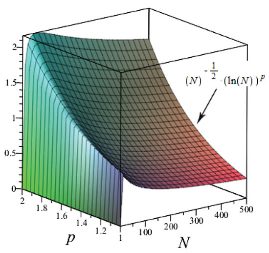
For $1\le p\le 2$, we know that $N^{-1/2}{(lnN)}^p\le c_7$ for some $c_7>0$; see Figure 3.

Figure 3. Graph of $y=N^{-1/2}{(lnN)}^p$ for $1\le p\le 2$.

Thus, the assertion can be obtained. □

4. Application to an Inverse Potential Problem

It is well known that an inverse potential problem is severely ill-posed. It is the problem of determining the shape of an unknown domain D from measurements of the Neumann boundary values of u on $\partial {\Omega }_R$ where the solution u fulfills Equations (1) and (2). In this work, Assumption 2.1 for the inverse potential problem cannot be presented. It fails even in the case of two concentric circles [2]. However, if we implement the method by representing the curve with a collocation basis, as will be seen in Proposition 3, the Fréchet derivative is reformulated. Without the verification of Assumption 1, we show a quite good performance of an approximated potential.

The nonlinear operator for an inverse potential problem is defined in the following form:

$$\begin{array}{cc}\hfill \left[F\left(x\right)\right]\left(t\right)& =\frac{1}{4\pi R}{\int }_0^{2\pi }{x}^2\left(s\right)\mathrm{ds}+\sum _{i=1}^{\infty }\frac{1}{\pi R^{i+1}(i+2)}{\int }_0^{2\pi }{x}^{i+2}\left(s\right)cos\left(is\right)\mathrm{ds}cos\left(it\right)\hfill \\ \hfill & +\sum _{i=1}^{\infty }\frac{1}{\pi R^{i+1}(i+2)}{\int }_0^{2\pi }{x}^{i+2}\left(s\right)sin\left(is\right)\mathrm{ds}sin\left(it\right)\hfill \end{array}$$

(69)

where $F:$$L^2[0,2\pi ]\to L^2[0,2\pi ]$. Moreover, the Fréchet derivative of the operator F is

$$\begin{array}{cc}\hfill \left[F^{\prime }\left(x\right)h\right]\left(t\right)& =\frac{1}{2\pi R}{\int }_0^{2\pi }x\left(s\right)h\left(s\right)\mathrm{ds}\hfill \\ & +\sum _{i=1}^{\infty }\frac{1}{\pi R^{i+1}}\left({\int }_0^{2\pi }{x}^{i+1}\left(s\right)h\left(s\right)cos\left(is\right)\mathrm{ds}cos\left(it\right)\right.\hfill \\ & \left.+{\int }_0^{2\pi }{x}^{i+1}\left(s\right)h\left(s\right)sin\left(is\right)\mathrm{ds}sin\left(it\right)\right),\hfill \end{array}$$

(70)

See Reference [1] for more details. In the presented work, we use $R=1$ and $x_0=\delta x^{+}\left(s\right)$. Since $X=L^2[0,2\pi ]$ and $Y=L^2[0,2\pi ]$, we discretized $[0,2\pi ]$ into m intervals with the grid points $0=t_0,t_1,\cdots ,t_m=2\pi$ and $0=s_0,s_1,\cdots ,s_m=2\pi$. Note that $X_m=\mathrm{span}\left\{{\phi }_j^{\left(m\right)}\right\}$ and $Y_m=\mathrm{span}\left\{{\psi }_j^{\left(m\right)}\right\}$, where the sets $\left\{{\phi }_1^{\left(m\right)}\cdots {\phi }_m^{\left(m\right)}\right\}$ and $\left\{{\psi }_1^{\left(m\right)}\cdots {\psi }_m^{\left(m\right)}\right\}$ are orthogonal bases. The orthogonal bases are defined with respect to the step length $h^{\left(m\right)}:=2\pi /m,m\in \mathbb{N}$ by the piecewise continuous function with ${\phi }_j^{\left(m\right)}\left(s\right)=1$ for $s\in [s_{j-1},s_j]$, ${\psi }_j^{\left(m\right)}\left(t\right)=1$ for $t\in [t_{j-1},t_j]$, and with ${\phi }_j^{\left(m\right)}\left(s\right)=0$, ${\psi }_j^{\left(m\right)}\left(t\right)=0$ otherwise. The result in the next proposition provides the formula for the calculation of $x_{n+1}^{\delta }$.

Proposition 3.

Let $x_n^{\delta }\left(s\right)={\sum }_{j=1}^m{u}_j^{\left(m\right)}{\phi }_j^{\left(m\right)}\left(s\right),x_{n+1}^{\delta }\left(s\right)={\sum }_{j=1}^m{v}_j^{\left(m\right)}{\phi }_j^{\left(m\right)}\left(s\right),$$x_0={\sum }_{j=1}^m{z}_j^{\left(m\right)}{\phi }_j^{\left(m\right)}\left(s\right)$ The coefficient vector $V^{\left(m\right)}$ is given by

$$\begin{array}{c}\hfill v_r^{\left(m\right)}=(1-{\alpha }_n)u_r^{\left(m\right)}+\frac{1}{h^{\left(m\right)}}{q}_r+{\alpha }_n{z}_r^{\left(m\right)}\end{array}$$

(71)

for $r=1,\dots ,m$, where

$$\begin{array}{cc}\hfill q_r& =h^{\left(m\right)}\sum _{k=1}^m\left[y_k^{\delta }\left(t_k\right)-C-\sum _{i=1}^{\infty }(D_{ki}+E_{ki})\right]\left[\frac{h^{\left(m\right)}}{4\pi }(x_n^{\delta }\left(s_{r-1}\right)+x_n^{\delta }\left(s_r\right))\right.\hfill \\ \hfill & +\sum _{i=1}^{\infty }\left(\frac{h^{\left(m\right)}}{2\pi }{A}_{ir}cos\left(i{t}_k\right)+\left.\frac{h^{\left(m\right)}}{2\pi }{B}_{ir}sin\left(i{t}_k\right)\right)\right],\hfill \end{array}$$

$$\begin{array}{cc}\hfill A_{ir}& ={\left(x_n^{\delta }\left(s_{r-1}\right)\right)}^{i+1}cos\left(s_{r-1}\right)+{\left(x_n^{\delta }\left(s_r\right)\right)}^{i+1}cos\left(i{s}_r\right),\hfill \\ \hfill B_{ir}& ={\left(x_n^{\delta }\left(s_{r-1}\right)\right)}^{i+1}sin\left(s_{r-1}\right)+{\left(x_n^{\delta }\left(s_r\right)\right)}^{i+1}sin\left(i{s}_r\right),\hfill \\ \hfill C& =\frac{h}{4\pi }\sum _{l=1}^m{\left(u_l^{\left(m\right)}\right)}^2,\hfill \\ \hfill D_{ki}& =\frac{h^{\left(m\right)}}{\pi (i+2)}\sum _{l=1}^m{\left(u_l^{\left(m\right)}\right)}^{i+2}cos\left(i{s}_l\right)cos\left(i{t}_k\right)\hfill \\ \hfill E_{ki}& =\frac{h^{\left(m\right)}}{\pi (i+2)}\sum _{l=1}^m{\left(u_l^{\left(m\right)}\right)}^{i+2}sin\left(i{s}_l\right)sin\left(i{t}_k\right).\hfill \end{array}$$

and

$$\begin{array}{c}\hfill z_r^{\left(m\right)}=\frac{h}{2}\left(x_0\left(s_{r-1}\right)+x_0\left(s_r\right)\right).\end{array}$$

Proof. 

The idea of the proof is analogous to Proposition 5 in Reference [21].  □

The numerical examples for recovering the potential $x^{+}$ are demonstrated in Figure 4, Figure 5 and Figure 6. We obtain data $y^{\delta }$ by solving the direct problem for the test curves. The program was written in MATLAB2018a. The results are demonstrated in Figure 4 and Figure 5 for the first test curve $x^{+}=\frac{5+sin\left(3s\right)}{6}$ and in Figure 6 for the second test curve $x^{+}=1-sin\left(s\right)$. For both examples, the number of basis functions is 65 and the number of equidistant grid points is 200. In Figure 4, ${\alpha }_n=\frac{1}{2}{(100+n)}^{-0.9},$$\delta =0.01$, and $\tau =120$ provide the error $0.4197$ with the residual norm $1.0792$ after 8 iterations for $i_{max}=3$ and the error $0.3911$ with the residual norm $1.1171$ after 8 iterations for $i_{max}=6$. In Figure 5, ${\alpha }_n=\frac{1}{2}{(100+n)}^{-0.9},\delta =0.001$, and $\tau =1100$ provide the error $0.6282$ with the residual error $1.0607$ after 8 iterations for $i_{max}=3$ and the error $0.5869$ with the residual norm $1.0993$ after 8 iterations for $i_{max}=6$. For the second example, ${\alpha }_n=\frac{1}{2}{(1000+n)}^{-0.9},\delta =0.01$, and $\tau =3000$ provide the error $0.5720$ with the residual norm $28.2597$ after 13 iterations and ${\alpha }_n=\frac{1}{2}{(1000+n)}^{-0.9},\delta =0.001$, and $\tau =1700$ provide the error $0.5925$ with the residual norm $15.4140$ after 14 iterations. Figure 4, Figure 5b,d, and Figure 6b show that the curve of $ln∥x^{+}-x_n^{\delta }∥$ lies below a straight line with slope $-p$ as suggested by Equation (29).

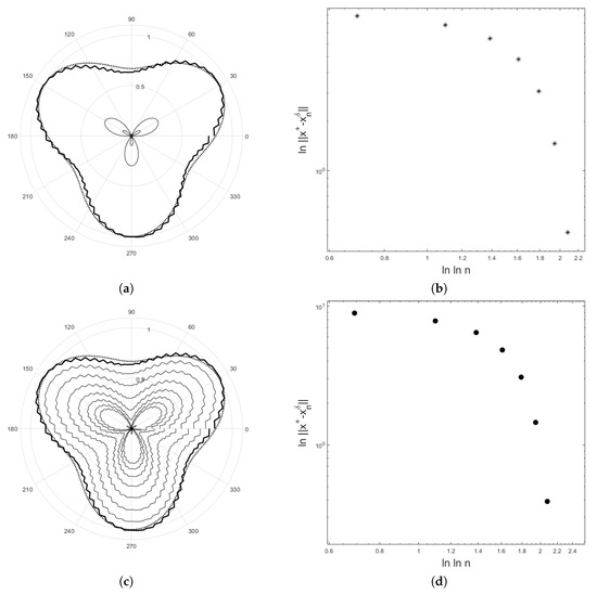
Figure 4. The polar plot shows the exact solution (dot line) and the computed solution (solid line) for (a) $i_{\max }=3$ and (c) $i_{\max }=6$ with $\delta =0.01$. In (a) the thin curve is an initial value. In (c) the thin curves are the curve of $x_n^{\delta }$ for $n=1,\dots ,8$. The error $\parallel x^{+}-x_n^{\delta }\parallel$ versus the logarithm of the number of iteration step using a double logarithm scale for (b) $i_{\max }=3$ and (d) $i_{\max }=6$ are shown. The initial value is $x_0$= $0.1+\frac{1}{5}sin\left(3s\right)$. The parameter ${\alpha }_n$ in Equation (71) is $\frac{1}{2}{(100+n)}^{-0.9}$.

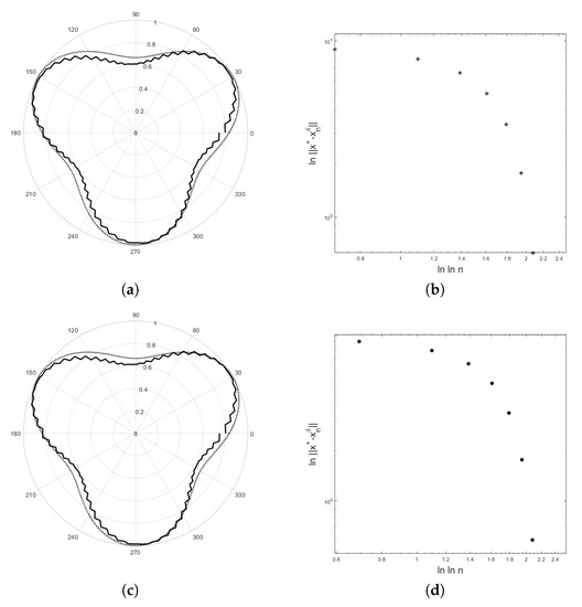
Figure 5. The polar plot shows the exact solution (dot line) and the computed solution (solid line) for (a) $i_{\max }=3$ and (c) $i_{\max }=6$ with $\delta =0.001$. The error $\parallel x^{+}-x_n^{\delta }\parallel$ versus the logarithm of the number of iteration step using a double logarithm scale for (b) $i_{\max }=3$ and (d) $i_{\max }=6$ are shown. The initial value is $x_0$= $0.1+\frac{1}{5}sin\left(3s\right)$. The parameter ${\alpha }_n$ in Equation (71) is $\frac{1}{2}{(100+n)}^{-0.9}$.

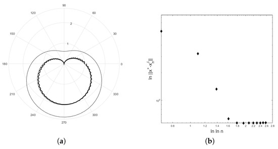
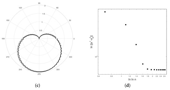
Figure 6. (a) The polar plot shows the exact solution (dot line) and the computed solution (solid line) for example 2 with (a,b) $\delta =0.01$ and (c,d) $0.001$. In (a), the thin curve is an initial value. The error $\parallel x^{+}-x_n^{\delta }\parallel$ versus the logarithm of the number of iteration step using a double logarithm scale is shown in (b) and (d). The initial value is $x_0$= $1.6-sin\left(s\right)$. The parameter ${\alpha }_n$ in Equation (71) is $\frac{1}{2}{(1000+n)}^{-0.9}$.

5. Conclusions

In this article, we show that the rate $O\left({(-ln\delta )}^{-p}\right)$ of the modified Landweber method in Equation (6) under the logarithmic source condition in Equation (7) with $1\le p\le 2$ is obtained. The regularization parameter was chosen according to the discrepancy principle. The linearity properties in Equations (17) and (18) of the nonlinear operator are needed although the verification for the inverse potential problem is not possible [2]. The test examples are used to illustrate the results in Theorem 1. For the modified Landweber regularization, the initial guess $x_0$ is an important information. With a good choice of initial guess, the shapes of the unknown domains D are quite good reconstructions. The curves in Figure 4, Figure 5b,d, and Figure 6b confirm the result in Theorem 1, where the curve of $ln∥x^{+}-x_n^{\delta }∥$ lies below a straight line with slope $-p$.

References

- Böckmann, C.; Kammanee, A.; Braunß, A. Logarithmic convergence rate of Levenberg–Marquardt method with application to an inverse potential problem. J. Inv. Ill-Posed Probl. 2011, 19, 345–367. [Google Scholar] [CrossRef]
- Hettlich, F.; Rundell, W. Iterative methods for the reconstruction of an inverse potential problem. Inverse Probl. 1996, 12, 251–266. [Google Scholar] [CrossRef]
- Hettlich, F.; Rundell, W. A second degree method for nonlinear inverse problems. SIAM J. Numer. Anal. 1999, 37, 587–620. [Google Scholar] [CrossRef]
- Van den Doel, K.; Ascher, U. On level set regularization for highly ill-posed distributed parameter estimation problems. J. Comput. Phys. 2006, 216, 707–723. [Google Scholar] [CrossRef][Green Version]
- Hohage, T. Logarithmic convergence rates of the iteratively regularized Gauss—Newton method for an inverse potential and an inverse scattering problem. Inverse Probl. 1997, 13, 1279. [Google Scholar] [CrossRef]
- Pornsawad, P.; Sapsakul, N.; Böckmann, C. A modified asymptotical regularization of nonlinear ill-posed problems. Mathematics 2019, 7, 419. [Google Scholar] [CrossRef]
- Tautenhahn, U. On the asymptotical regularization of nonlinear ill-posed problems. Inverse Probl. 1994, 10, 1405–1418. [Google Scholar] [CrossRef]
- Zhang, Y.; Hofmann, B. On the second order asymptotical regularization of linear ill-posed inverse problems. Appl. Anal. 2018. [Google Scholar] [CrossRef]
- Pornsawad, P.; Böckmann, C. Modified iterative Runge-Kutta-type methods for nonlinear ill-posed problems. Numer. Funct. Anal. Optim. 2016, 37, 1562–1589. [Google Scholar] [CrossRef]
- Mahale, P.; Nair, M. Tikhonov regularization of nonlinear ill-posed equations under general source condition. J. Inv. Ill-Posed Probl. 2007, 15, 813–829. [Google Scholar] [CrossRef]
- Romanov, V.; Kabanikhin, S.; Anikonov, Y.; Bukhgeim, A. Ill-Posed and Inverse Problems: Dedicated to Academician Mikhail Mikhailovich Lavrentiev on the Occasion of his 70th Birthday; De Gruyter: Berlin, Germany, 2018. [Google Scholar]
- Scherzer, O. A modified Landweber iteration for solving parameter estimation problems. Appl. Math. Optim. 1998, 38, 45–68. [Google Scholar] [CrossRef]
- Deuflhard, P.; Engl, W.; Scherzer, O. A convergence analysis of iterative methods for the solution of nonlinear ill-posed problems under affinely invariant conditions. Inverse Probl. 1998, 14, 1081–1106. [Google Scholar] [CrossRef]
- Bakushinsky, A.; Kokurin, M.; Kokurin, M. Regularization Algorithms for Ill-Posed Problems; Inverse and Ill-Posed Problems Series; De Gruyter: Berlin, Germany, 2018. [Google Scholar]
- Schuster, T.; Kaltenbacher, B.; Hofmann, B.; Kazimierski, K. Regularization Methods in Banach Spaces; Radon Series on Computational and Applied Mathematics; De Gruyter: Berlin, Germany, 2012. [Google Scholar]
- Albani, V.; Elbau, P.; de Hoop, M.V.; Scherzer, O. Optimal convergence rates results for linear inverseproblems in Hilbert spaces. Numer. Funct. Anal. Optim. 2016, 37, 521–540. [Google Scholar] [CrossRef] [PubMed][Green Version]
- Kaltenbacher, B.; Neubauer, A.; Scherzer, O. Iterative Regularization Methods for Nonlinear Ill-Posed Problems; De Gruyter: Berlin, Germany; Boston, MA, USA, 2008. [Google Scholar]
- Louis, A.K. Inverse und Schlecht Gestellte Probleme; Teubner Studienbücher Mathematik, B. G. Teubner: Stuttgart, Germany, 1989. [Google Scholar]
- Vainikko, G.; Veterennikov, A.Y. Iteration Procedures in Ill-Posed Problems; Nauka: Moscow, Russia, 1986. [Google Scholar]
- Hanke, M.; Neubauer, A.; Scherzer, O. A convergence analysis of the Landweber iteration for nonlinear ill-posed problems. Numer. Math. 1995, 72, 21–37. [Google Scholar] [CrossRef]
- Böckmann, C.; Pornsawad, P. Iterative Runge-Kutta-type methods for nonlinear ill-posed problems. Inverse Probl. 2008, 24, 025002. [Google Scholar] [CrossRef][Green Version]
© 2020 by the authors. Licensee MDPI, Basel, Switzerland. This article is an open access article distributed under the terms and conditions of the Creative Commons Attribution (CC BY) license (http://creativecommons.org/licenses/by/4.0/).