Dynamic Pricing and Optimal Control for a Stochastic Inventory System with Non-Instantaneous Deteriorating Items and Partial Backlogging

Abstract

In this paper, we consider a problem of the dynamic pricing and inventory control for non-instantaneous deteriorating items with uncertain demand, in which the demand is price-sensitive and governed by a diffusion process. Shortages and remains are permitted, and the backlogging rate is variable and dependent on the waiting time for the next replenishment. In order to maximize the expected total profit, the problem of dynamic pricing and inventory control is described as a stochastic optimal control problem. Based on the dynamic programming principle, the stochastic control model is transformed into a Hamilton-Jacobi-Bellman (HJB) equation. Then, an exact expression for the optimal dynamic pricing strategy is obtained via solving the HJB equation. Moreover, the optimal initial inventory level, the optimal selling pricing, the optimal replenishment cycle and the optimal expected total profit are achieved when the replenishment cycle starts at time 0. Finally, some numerical simulations are presented to demonstrate the analytical results, and the sensitivities analysis on system parameters are carried out to provide some suggestions for managers.

1. Introduction

The deterioration, including the spoilage, damage, dryness, loss of utility, is commonly observed in physical goods, for example food stuffs, electronic products, medicine, and so on. It’s essential and critical for the business manager to achieve well-managed inventory of deteriorating items, and this has come to the attention of many researchers.

Ghare and Schrader (1963) [1] first developed an optimal ordering policy for deteriorating items and proposed an Economic Order Quantity (EOQ) model with a negative exponentially decaying inventory. Covert and Philip (1973) [2] studied an inventory model with the assumption that the deterioration time follows a two-parameter Weibull distribution. Shah (1977) [3] considered a deterministic inventory model with the condition that shortage is permitted. Recently, Goyal and Giri (2001) [4] offered a detailed review of reported literatures about deteriorating inventory. Bakker, Riezebos and Teunter (2012) [5] conducted a survey on work reported about inventory systems with deterioration.

The problem lies in the above mentioned literatures is that, almost all researchers assume that the deterioration starts upon arrival at the inventory. However, in reality, this does not always apply and this misconception may lead the retailer to make inappropriate replenishment policies. For example, some goods, such as firsthand fruits and vegetables, can keep their original quality or condition for some time. In other words, deterioration does not occur during this period. The concept of “non-instantaneous deterioration” was brought up by Wu, Ouyang and Yang (2006) [6]. They considered a problem of optimal replenishment policy for non-instantaneous deteriorating items with stock-dependent demand. Ouyang, Wu and Yang (2006) [7] established an appropriate inventory model for non-instantaneous deteriorating items with permissible delay in payments. Chang and Lin (2010) [8] derived an inventory model for non-instantaneous deteriorating items with stock-dependent demand rate under inflation over a finite planning horizon.

The price fluctuates as the time goes and has an impact on the demand, incorporating the variable of selling price into the inventory policies have been widely adopted in some recent research. Whitin (1955) [9] first considered the selling price as the decision variable in the basic EOQ model. Wee (1997) [10] raised an optimal replenishment policy for deterioration inventory in which the demand is a linear function of price. Moreover, Wu, Ouyang and Yang (2009) [11] established an applicable inventory system exposed to the price-sensitive demand, and obtained the optimal selling price and the length of replenishment cycle. Soni and Patel (2013) [12] studied a model for non-instantaneous deteriorating items with imprecise deterioration free time and credibility constraint, which assumes that time and price are dependent on demand when deterioration occurs. Zhang et al. (2015) [13] considered the optimal dynamic pricing strategy and replenishment cycle for non-instantaneous items, in which the demand depends on the sale price and the items’ quantity. Duan, Cao and Huo (2018) [14] studied a joint dynamic pricing and production decisions for deteriorating items with price-dependent stochastic demand, and achieved the closed-form solutions by dynamic programming principle. Li, Zhang and Han(2017) [15] considered the dynamic pricing and periodic ordering for deteriorating items with uncertain demand dependent on the selling price and the inventory level, in which the stochastic control model is transformed into a HJB equation. Other researchers in the related domain area include Geetha and Udayakumar (2016) [16], Das et al. (2020) [17], Debata and Acharya (2017) [18], and Agi and Soni (2020) [19], etc.

In addition, shortage is another significant factor for business managers to consider in making the optimal inventory control policy. When shortages occur, some customers would like to wait for backlogging while the others may give up waiting and turn to alternatives. The willingness to accept backlogging is determined by the length of waiting time for the next replenishment. In other words, the backlogging rate depends on the waiting time. Chang and Dye (1999) [20] considered an EOQ model which allows shortage and partially backlogged. The backlogging rate is assumed to be a decreasing function of the waiting time for the next replenishment. Maihami and Kamalabadi (2012) [21] studied a joint pricing and inventory control for non-instantaneous deteriorating items allowing shortages and partially backlogged. Furthermore, Soni and Suthar (2018) [22] investigated an inventory system for non-instantaneous deteriorating items with partially backlogged wherein the demand is stochastic in nature and price-dependent. The other works on inventory systems with partially backlogged have been reported by Abad (2001) [23], Wang (2002) [24], Dye, Ouyang and Hsieh (2007) [25], Papachristos and Skouri (2003) [26], and Farughi, Khanlarzade and Yegane (2014) [27], etc.

It is noted that the demand of inventory system with non-instantaneous deteriorating items is almost assumed to a deterministic function in the previous works. However, in practice, the demand is stochastic because of the volatility of the market. Therefore, in order to give a better description of realistic circumstances, a problem of the dynamic pricing and optimal control for a stochastic inventory system with non-instantaneous deteriorating items is considered in this study. The demand is price-sensitive and governed by a diffusion process. Note that the cumulative demand process is quite different from [22] in which the stochastic component of the cumulative demand is a non-negative, continuous random variable independent of time. Shortages and surplus are allowed, and the backlogging rate is variable and dependent on the waiting time for the next replenishment. Then, the problem of achieving the optimal pricing is transformed to solve a HJB equation according to the dynamic programming principle. And, an exact expression of the optimal pricing strategy is obtained. Furthermore, the influence of volatility of the potential demand on profit is analysed. The optimal initial inventory level, the optimal selling price, the optimal replenishment cycle and the optimal total expected profit are achieved when the replenishment starts at time 0. Finally, some numerical experiments are presented to illustrate the developed model. The sensitivities analysis of the optimal solutions with respect to the system parameters are performed to give more managerial insights.

The rest of this paper is organized as follows. In Section 2, the notations and assumptions are presented. In Section 3, we formulate the model by considering the possible costs and revenues, and present a problem of stochastic optimal control. In Section 4, the optimal selling pricing, the optimal initial inventory level, the optimal replenishment cycle and the optimal expected total profit are obtained based on the stochastic optimal control method. In Section 5, we provide some numerical experiments and sensitivities analysis on some major system parameters to demonstrate the effectiveness of the achieved analytical solutions. In Section 6, the conclusions are presented.

2. Notations and Assumptions

The following notations and assumptions are used in this paper:

Notations:

• c: the constant purchasing cost per unit, $c>0$.
• h: the holding cost per unit per unit time, $h>0$.
• C: the ordering cost per replenishment cycle, which is independent of the order quantity, $C>0$.
• $\theta$: the deterioration rate, $\theta >0$.
• T: the duration of a replenishment cycle, such as one week, one month, one quarter, $T<\infty$.
• $t_d$: the length of time where items exhibit no deterioration.
• $x_0$: the initial inventory level, $x_0\ge 0$.
• $X(t)$: the inventory level at time t.
• $p(t)$: the selling price per unit at time t.
• $\alpha$: the demand sensitivity to the selling price, $\alpha <0$.
• b: the fixed term of demand rate determined by the market size, $b>0$.
• $dW$: the increment of standard Brownian process.
• $\sigma$: the volatility of the potential demand, $\sigma >0$.
• $\gamma$: punishment coefficient when stock-out, $\gamma >0$.
• S: the maximum inventory level, $S>0$.
• $\mathsf{\Omega }$: the admissible control set.
• $F(p(·))$: the profit function.
• $V(t,X(t);T)$: the value function.
• $p^{*}(t)$: the optimal selling price at time t.
• $T^{*}$: the optimal replenishment cycle.
• $x_0^{*}$: the optimal initial inventory level.
• $V^{*}$: the optimal expected total profit.

Assumptions:

• A single non-instantaneous deteriorating item is assumed.
• The selling price changes over time and needs to be determined by the retailer.
• The lead time is zero and the replenishment rate is infinite.
• The cumulative demand $D(t)$ is a stochastic process governed by a diffusion process

  $$\begin{array}{c}\hfill dD(t)=(b+\alpha p(t))dt+\sigma dW(t),\end{array}$$

  (1)

  which is dependent on the selling price $p(t)$. The mean market potential b can be understood as the maximum sales when the items are free. The term $\sigma dW(t)$ represents the fluctuation of the demand due to the uncertainty of the environment. Note that the notion of “demand” is in a rather broad sense: Any withdrawal from or addition to the inventory can be regarded as an action of the demand. Therefore, it may cover those processes such as inventory spoilage and sales return, which are in general quite random. Moreover, we always assume that $b+\alpha c>0$ holds, otherwise there is no market for this item.
• The inventory level is influenced by the deterioration rate and demand. If $t\in [0,t_d]$, the items exhibit no deterioration. If $t\in [t_d,T]$, we assume the deterioration rate is a constant and the amount of deteriorating items at time t are $\theta X(t)$.
• Shortages are allowed. We assume that during the period of shortages, the retailer will not lose his customers completely who are not satisfied with the retailer. Besides, when $X(t)=0$ $(t<T)$, the backlogging rate depends on the delay between the confirmation of the customer order and the next replenishment. Thus, the demand is partially backlogged according to the fraction $e^{-\gamma (T-t)}$.
• Remains are allowed. We assume that when $X(T)>0$, the retailer should pay the penalties $r{X}^2(T)$ at the end of the replenishment cycle T. It should be noted that the quadratic convex function of surplus cost captures the increasing marginal cost, which is in accord with reported articles (see, e.g., [14,28]). In fact, numerous greengrocers may discard substandard items when the next replenishment cycle arrives. Thus, it is reasonable to assume that the penalties should be paid if there are remains.
• There is no replacement or repair of the deterioration items.
• In real life, the shelf space is limited in many retail outlets. Thus, we impose a maximum inventory level S, that is, $X(t)\le S$, for all $t\in [0,T]$.

3. The Model Formulation

The stochastic inventory system is described as follows: The replenishment cycle starts at time 0 and ends at time T, during which there is no other replenishment. At the beginning of a cycle, there are $x_0$ units of item arriving at the system. When the items exhibit on deterioration, the inventory level $X(t)$ decreases only due to the uncertainty of demand. When the items start to deteriorate, the inventory level $X(t)$ falls resulting from the uncertain demand and the deterioration rate. Shortages occur if $X(t)=0$ for $t<T$ and remains occur if $X(T)>0$.

On the basis of above discuss, the status of inventory level at any time t is governed by the following stochastic differential equation:

$$\begin{array}{c}\hfill \left\{\begin{array}{cc}dX(t)\hfill & =-\theta X(t)I_{t\ge t_d}-dD(t)\hfill \\ & =(-\theta X(t)I_{t\ge t_d}-(b+\alpha p(t)))dt+\sigma dW(t),\hfill \\ X(0)\hfill & =x_0,\hfill \end{array}\right.\end{array}$$

(2)

where $x_0$ is the initial inventory level. For all $t\in [0,T]$, $I_{t\ge t_d}=1$ if $t\ge t_d$, otherwise, $I_{t\ge t_d}=0$.

During the time interval $[t,t+dt)$, the instantaneous change of the inventory level $dX(t)$ is divided into two parts. The stochastic component $\sigma dW(t)$ describes the potential market demand. The deterministic component $(-\theta X(t)I_{t\ge t_d}-(b+\alpha p(t)))dt$ represents the expected change in inventory level. After the current time t, the moment of items sold out before next replenishment is denoted by $\tau$ ([15]), that is, $X(\tau )=0$, $\tau <T$, otherwise $\tau =T$, indicating that there has remaining stock. Therefore, it can be described as:

$$\begin{array}{c}\hfill \tau =inf\left\{s>t:(s,X(s))\notin (0,T)\times (0,S)\right\}.\end{array}$$

Now, we can obtain all the relevant costs and sales revenues per replenishment cycle, which consists of the following components:

• The ordering cost per cycle is represented by C.
• The inventory holding cost is presented by

  $$\begin{array}{c}\hfill h{\int }_0^{\tau }X(t)dt.\end{array}$$
• The surplus cost is $r{X}^2(T)$, where $X(T)>0$.
• The profit on sale is presented by

  $$\begin{array}{c}\hfill {\int }_0^{\tau }(p(t)-c)dD(t)={\int }_0^{\tau }[p(t)-c][b+\alpha p(t)]dt+{\int }_0^{\tau }[p(t)-c]\sigma dW(t).\end{array}$$
• During the shortage period $[\tau ,T]$, i.e., $X(\tau )=0$, the profit is represented by

  $$\begin{array}{c}\hfill {\int }_{\tau }^T[p(t)-c]e^{-\gamma (T-t)}dD(t)={\int }_{\tau }^T[p(t)-c][b+\alpha p(t)]e^{-\gamma (T-t)}dt+{\int }_{\tau }^T[p(t)-c]e^{-\gamma (T-t)}\sigma dW(t).\end{array}$$
  In this period, the retailer can make orders, but cannot make delivery at once. Since the delivery is delayed, the demand rate is

  $$\begin{array}{c}\hfill e^{-\gamma (T-t)}dD(t),\end{array}$$

  which depends on the delay time length $T-t$.

According to the above components, the profit function is then specified as

$$\begin{array}{c}\hfill \begin{array}{cc}\hfill F(p(·))& =E\{{\int }_0^{\tau }[p(t)-c][b+\alpha p(t)]dt\hfill \\ & -{\int }_0^{\tau }hX(t)dt+{\int }_{\tau }^T[p(t)-c][b+\alpha p(t)]e^{-\gamma (T-t)}dt-r{X}^2(T)\}-C.\hfill \end{array}\end{array}$$

(3)

Without loss of generality, we assume that there is no discounting in (3). It is noted that the selling price $p(t)$ satisfies $0\le p(t)\le \frac{b}{-\alpha }$, whose upper bound origins from the fact that the demand rate should remain non-negative. Thus, the admissible control set is

$$\begin{array}{c}\hfill \mathsf{\Omega }=\left\{p(t)|p(t)\in [0,\frac{b}{-\alpha }]\right\}.\end{array}$$

In order to maximize the total expected net profit over the replenishment cycle T, the retailer should find an optimal selling price. Let $J_p(t,x)$ be the expected profit function from t to T without ordering cost

$$\begin{array}{ccc}\hfill J_p(t,x)& =& E\left[{\int }_t^{\tau }(p(s)-c)(b+\alpha p(s))ds-{\int }_t^{\tau }hX(s)ds\right.\hfill \\ & & \left.+{\int }_{\tau }^T(p(s)-c)(b+\alpha p(s))e^{-\gamma (T-s)}ds-r{X}^2(T)|X(t)=x\right].\hfill \end{array}$$

The stochastic optimal control problem is to maximize $J_p(t,x)$ over all $p(·)\in \mathsf{\Omega }$, i.e., we need to seek $p^{*}(·)\in \mathsf{\Omega }$ such that

$$\begin{array}{c}\hfill J_{p^{*}}(t,x)=\underset{p\in \mathsf{\Omega }}{sup}{J}_p(t,x).\end{array}$$

(4)

4. Optimal Control Analysis

We define the value function $V(t,x;T)$ of the stochastic optimal control problem (4) by

$$\begin{array}{c}\hfill V(t,x;T)=J_{p^{*}}(t,x).\end{array}$$

(5)

Then, we analyze the boundary conditions of $V(t,x;T)$. When $X(t)=0$ for $t\in [0,T]$, the shortages occur, and the retailer should make the optimal selling price $\overline{p}$ in order to maximize the expected profit. By maximizing the profit during the shortage period, the optimal selling price is given by

$$\begin{array}{c}\hfill \overline{p}=\frac{b-\alpha c}{-2\alpha }\end{array}$$

and the profit $V(t,0;T)$ is presented by

$$\begin{array}{c}\hfill V(t,0;T)={\int }_{\tau }^T(\overline{p}-c)(b+\alpha \overline{p})e^{-\gamma (T-t)}dt=\frac{{(b+\alpha c)}^2}{-4\alpha }\frac{1-e^{-\gamma (T-\tau )}}{\gamma }.\end{array}$$

(6)

When $X(T)>0$, the remains occur, and the retailer should pay the surplus cost $r{X}^2(T)$. Thus, we have

$$\begin{array}{c}\hfill V(T,x;T)=-r{x}^2.\end{array}$$

(7)

Let $f:\mathbb{R}\times \mathbb{R}\times \mathsf{\Omega }\mapsto \mathbb{R}$ be a given continuous function called “profit rate” function defined as follows:

$$\begin{array}{c}\hfill f(t,x,p)=(p-c)(b+\alpha p)-hx-c\theta I_{t\ge t_d}x.\end{array}$$

(8)

By the dynamic programming principle, we have the following HJB equation

$$\begin{array}{c}\hfill -V_t=\underset{p\in \mathsf{\Omega }}{max}[f(t,x,p)+(-\theta x{I}_{t\ge t_d}-(b+\alpha p))V_x+\frac{{\sigma }^2}{2}{V}_{xx}]\end{array}$$

(9)

with the boundary condition (6) and (7) on $(0,T)\times \left\{0\right\}$ and $\left\{T\right\}\times (0,S)$, respectively, where $V_x=\partial V/\partial x$, $V_{xx}={\partial }^{2}V/\partial x^2$, $V_t=\partial V/\partial t$.

Maximizing of (9) with respect to the selling price p results in an optimal control

$$\begin{array}{c}\hfill p^{*}(t)=\left\{\begin{array}{cc}0,\hfill & \mathrm{if}{V}_x<-\frac{b-\alpha c}{-\alpha },\hfill \\ \frac{b-\alpha c}{-2\alpha }+\frac{V_x}{2},\hfill & \mathrm{if}{V}_x\ge -\frac{b-\alpha c}{-\alpha }.\hfill \end{array}\right.\end{array}$$

(10)

The optimal selling price $p^{*}(t)$ is an interior solution if $V_x\ge -\frac{b-\alpha c}{-\alpha }$. Otherwise, $p^{*}(t)=0$, which is a boundary solution. To determine an interior solution, we substitute $p^{*}(t)=\frac{b-\alpha c}{-2\alpha }+\frac{V_x}{2}$ into (9), which leads to

$$\begin{array}{c}\hfill a_1{(V_x)}^2+(-\theta x{I}_{t\ge t_d}-\frac{b+\alpha c}{2})V_x+a_2{V}_{xx}+V_t-(h+c\theta I_{t\ge t_d})x+a_3=0\end{array}$$

(11)

where

$$\begin{array}{c}\hfill a_1=\frac{-\alpha }{4},a_2=\frac{{\sigma }^2}{2},a_3=-\frac{{(b-\alpha c)}^2}{4\alpha }-bc.\end{array}$$

To solve the above (11), we set

$$\begin{array}{c}\hfill V(t,x;T)=A(t)x^2+B(t)x+C(t).\end{array}$$

(12)

According to the final condition $V(T,x;T)=-r{x}^2$, we have that

$$\begin{array}{c}\hfill A(T)=-r,B(T)=0,C(T)=0.\end{array}$$

(13)

Taking the partial derivatives of t and x in (12), we get

$$\begin{array}{c}{V}_x=2A(t)x+B(t),\hfill \end{array}$$

(14)

$$\begin{array}{c}{V}_{xx}=2A(t),\hfill \end{array}$$

(15)

$$\begin{array}{c}{V}_t=\dot{A}(t)x^2+\dot{B}(t)x+\dot{C}(t),\hfill \end{array}$$

(16)

where $\dot{A}(t)=dA(t)/dt$, $\dot{B}(t)=dB(t)/dt$, $\dot{C}(t)=dC(t)/dt$. Substituting (14)–(16) into the left-hand side of (11), we have

$$\begin{array}{c}\hfill (4a_1{A}^2-2\theta I_{t\ge t_d}A+\dot{A})x^2+(4a_{1}AB-\theta I_{t\ge t_d}B-(b+\alpha c)A\\ \hfill +\dot{B})x-(h+c\theta I_{t\ge t_d})x+a_1{B}^2-\frac{b+\alpha c}{2}B+\dot{C}+2a_{2}A+a_3=0,\end{array}$$

which should hold for any x.

If $t\in [t_d,T]$, i.e., $dX(t)=(-\theta X(t)-(b+\alpha p(t)))dt+\sigma dW(t)$, using the boundary condition (13), we achieve the following differential equations:

$$\begin{array}{c}\dot{A}=2\theta A-4a_1{A}^2,A(T)=-r,\hfill \end{array}$$

(17)

$$\begin{array}{c}\dot{B}=\theta B+(b+\alpha c)A+(h+c\theta )-4a_{1}AB,B(T)=0,\hfill \end{array}$$

(18)

$$\begin{array}{c}\dot{C}=\frac{b+\alpha c}{2}-a_1{B}^2-2a_{2}A-a_3,C(T)=0.\hfill \end{array}$$

(19)

Solving (17) (See Appendix A for details), we obtain

$$\begin{array}{c}\hfill A(t)=\frac{\theta }{-\alpha }+\frac{\theta }{-\alpha }\frac{k{e}^{2\theta (t-T)}-1}{k{e}^{2\theta (t-T)}+1},\end{array}$$

(20)

where $m=-r-\frac{\theta }{-\alpha }$ and $k=\frac{\theta -\alpha m}{\theta +\alpha m}<0$.

Substituting (20) into (18) and solving (18) (See Appendix B for details), yield

$$\begin{array}{c}\hfill B(t)=\frac{e^{\theta t}}{k{e}^{2\theta (t-T)}+1}\tilde{c}+(\frac{2(b+\alpha c)}{-\alpha }+\frac{h+c\theta }{\theta })\frac{k{e}^{2\theta (t-T)}}{k{e}^{2\theta (t-T)}+1}-\frac{h+c\theta }{\theta }\frac{1}{k{e}^{2\theta (t-T)}+1}\end{array}$$

(21)

where

$$\begin{array}{c}\hfill \tilde{c}=-k(\frac{2(b+\alpha c)}{-\alpha }+\frac{h+c\theta }{\theta })e^{-\theta T}+\frac{h+c\theta }{\theta }{e}^{-\theta T}.\end{array}$$

Based on the solution $A(t)$ and $B(t)$, we obtain the general solution of (19)

$$\begin{array}{c}\hfill C(t)=-{\int }_t^T(\frac{b+\alpha c}{2}B(t)-a_1{B}^2(t)-2a_{2}A(t)-a_3)dt.\end{array}$$

Substituting coefficients (20) and (21) in the derivative of the value function $V_x=2A(t)x+B(t)$, the interior optimal solution defined by (10) is obtained.

Similarly, if $t\in [0,t_d]$, that is, $dX(t)=(-(b+\alpha p(t)))dt+\sigma dW(t)$, setting $V=A_1{x}^2+B_{1}x+C_1$, we have

$$\begin{array}{c}{\dot{A}}_1=-4a_1{A}_1^2,A_1(T)=-r,\hfill \\ {\dot{B}}_1=(b+\alpha c)A_1+h-4a_1{A}_1{B}_1,B_1(T)=0,\hfill \\ {\dot{C}}_1=\frac{b+\alpha c}{2}-a_1{B}_1^2-2a_2{A}_1-a_3,C_1(T)=0.\hfill \end{array}$$

The solutions to this system (see Appendix C for details) are given by

$$\begin{array}{c}{A}_1(t)=\frac{r}{-\alpha r(t-T)-1},\hfill \\ B_1(t)=\frac{1}{-\alpha r(t-T)-1}\widetilde{c_1}+(b+\alpha c)\frac{rt}{-\alpha r(t-T)-1}+h\frac{-\alpha r{t}^2+2\alpha rtT-2t}{2(-\alpha r(t-T)-1)},\hfill \\ C_1(t)=-{\int }_t^T(\frac{b+\alpha c}{2}{B}_1(t)-a_1{B}_1^2(t)-2a_2{A}_1(t)-a_3)dt,\hfill \end{array}$$

where

$$\begin{array}{c}\hfill \widetilde{c_1}=-(b+\alpha c)rT+h(\frac{-\alpha }{2}r{T}^2+T).\end{array}$$

Similarly, substituting coefficients $A_1(t)$ and $B_1(t)$ in the derivative of the value function $V_x=2A_1(t)+B_1(t)$, the interior optimal solution defined by (10) is achieved.

According to the above analysis, the following proposition can be obtained.

Proposition 1.

For the given parameters r, θ, α,

(1) 

$A(t)$ and $A_1(t)$ are decreasing with respect to t strictly. Moreover, when $0\le t<T$, $A(t)$ and $A_1(t)$ are negative;

(2) 

As the increasing in the volatility of the potential demand σ, V is decreasing.

Proof of Proposition 1.

For case (1), it is obviously that when $0\le t<T$, $A(t)$ and $A_1(t)$ are negative from the expressions of the solution $A(t)$ and $A_1(t)$. Calculating the first order derivative of $A(t)$ and $A_1(t)$, we have

$$\begin{array}{c}\dot{A}(t)=\frac{{\theta }^2}{a_1}\frac{k{e}^{2\theta (t-T)}}{{(k{e}^{2\theta (t-T)}+1)}^2}<0,\hfill \\ \dot{A_1}(t)=-4a_1{(\frac{r}{4a_{1}r(t-T)-1})}^2<0.\hfill \end{array}$$

Thus, $A(t)$ and $A_1(t)$ are strictly decreasing in t.

For case (2), taking the first-order derivative of V with respect to $\sigma$, we have

$$\begin{array}{c}\frac{dV}{d\sigma }=2\sigma {\int }_t^{T}A(s)ds<0,ift\in [t_d,T),\hfill \\ \frac{dV}{d\sigma }=2\sigma {\int }_t^T{A}_1(s)ds<0,ift\in [0,t_d].\hfill \end{array}$$

Therefore, V is decreasing as the increasing in the volatility of the potential demand $\sigma$. The proof is completed. □

Proposition 1.(1) shows $A(t)$ and $A_1(t)$ are monotonically decreasing. $V(t,x;T)$ is concave and the optimal expected profit is existing based on the negativity of both $A(t)$ and $A_1(t)$. Furthermore, it can be seen from Proposition 1.(2) that $V(t,x;T)$ decreases with respect to the volatility of the potential demand, that is, a higher volatility of the potential demand always results in a lower expected total profit. This is in line with the actual situation.

Substituting the obtained polynomial solution into (10), the optimal pricing $p^{*}(t)$ for the stochastic control problem (4) without constraints are given in the following lemma.

Lemma 1.

If the control process $p(·)$ has no constraint,

(1) 

for $t_d\le t<T$, the optimal selling price $p^{*}(t,X(t))$ is presented by

$$\begin{array}{c}\hfill p^{*}(t,X(t))=\left\{\begin{array}{cc}\frac{2\theta }{-\alpha }\frac{k{e}^{2\theta (t-T)}}{k{e}^{2\theta (t-T)}+1}X(t)+\frac{(k{k}_1{e}^{\theta (t-T)}+k_2)(e^{\theta (t-T)}-1)}{2(k{e}^{2\theta (t-T)}+1)}+\frac{b-\alpha c}{-2\alpha },\hfill & \mathit{if}X(t)>0,\hfill \\ \frac{b-\alpha c}{-2\alpha },\hfill & \mathit{if}X(t)=0,\hfill \end{array}\right.\end{array}$$

(22)

where $k_1=\frac{2(b+\alpha c)}{-\alpha }+\frac{h+c\theta }{\theta }>0$, $k_2=\frac{h+c\theta }{\theta }>0$.

(2) 

for $0\le t\le t_d$, the optimal selling price $p^{*}(t,X(t))$ is given by

$$\begin{array}{c}\hfill p^{*}(t,X(t))=\left\{\begin{array}{cc}\frac{r}{-\alpha r(t-T)-1}X(t)+\frac{(2k_{3}r+h(-\alpha r(t-T)-2))(t-T)}{4(-\alpha r(t-T)-1)}+\frac{b-\alpha c}{-2\alpha },\hfill & \mathit{if}X(t)>0,\hfill \\ \frac{b-\alpha c}{-2\alpha },\hfill & \mathit{if}X(t)=0,\hfill \end{array}\right.\end{array}$$

(23)

where $k_3=b+\alpha c>0$.

In practice, the selling price $p(t)$ and the demand rate should be non-negative, resulting in $0\le p^{*}(t,X(t))\le \frac{b}{-\alpha }$. Based on Lemma 1, the optimal selling price $p^{*}(t,X(t))$ for the stochastic control problem (4) under above constraint is presented in the following theorem.

Theorem 1.

For the joint dynamic pricing and inventory control problem (4),

(1) 

if $0\le t<t_d$, then the optimal selling price $p^{*}(t,X(t))$ is given by

$$\begin{array}{c}\hfill \begin{array}{c}\hfill p^{*}(t,X(t))=\left\{\begin{array}{cc}\frac{b-\alpha c}{-2\alpha },\hfill & ifX(t)=0,\hfill \\ \frac{b}{-\alpha },\hfill & ifX(t)\le X_{min,1},\hfill \\ 0,\hfill & ifX(t)\ge X_{max,1},\hfill \\ \frac{r}{-\alpha r(t-T)-1}X(t)+\frac{(2k_{3}r+h(-\alpha r(t-T)-2))(t-T)}{4(-\alpha r(t-T)-1)}+\frac{b-\alpha c}{-2\alpha },\hfill & if{X}_{min,1}<X(t)<X_{max,1},\hfill \end{array}\right.\end{array}\end{array}$$

(24)

where $X_{min,1}=\frac{-1}{A_1}(\frac{B_1}{2}-\frac{b+\alpha c}{-2\alpha })$, $X_{max,1}=\frac{-1}{A_1}(\frac{B_1}{2}+\frac{b-\alpha c}{-2\alpha })$;

(2) 

if $t_d\le t<T$, then the optimal selling price $p^{*}(t,X(t))$ is given by

$$\begin{array}{c}\hfill \begin{array}{c}\hfill p^{*}(t,X(t))=\left\{\begin{array}{cc}\frac{b-\alpha c}{-2\alpha },\hfill & ifX(t)=0,\hfill \\ \frac{b}{-\alpha },\hfill & ifX(t)\le X_{min,2},\hfill \\ 0,\hfill & ifX(t)\ge X_{max,2},\hfill \\ \frac{2\theta }{-\alpha }\frac{k{e}^{2\theta (t-T)}}{k{e}^{2\theta (t-T)}+1}X(t)+\frac{(k{k}_1{e}^{\theta (t-T)}+k_2)(e^{\theta (t-T)}-1)}{2(k{e}^{2\theta (t-T)}+1)}+\frac{b-\alpha c}{-2\alpha },\hfill & if{X}_{min,2}<X(t)<X_{max,2},\hfill \end{array}\right.\end{array}\end{array}$$

(25)

where $X_{min,2}=\frac{-1}{A}(\frac{B}{2}-\frac{b+\alpha c}{-2\alpha })$, $X_{max,2}=\frac{-1}{A}(\frac{B}{2}+\frac{b-\alpha c}{-2\alpha })$.

Proof of Theorem 1.

According to (22)–(23) of Lemma 1 and $0\le p^{*}(t,X(t))\le \frac{b}{-\alpha }$, we obtain the above theorem. □

Theorem 1 indicates the optimal selling price $p^{*}(t,X(t))$ is a linear decreasing function of $X(t)$, providing the relationships of qualitative and quantitative between decision variable and system parameters. It is worth noting that the inventory system we construct is stochastic, however, when given $X(t)$, the optimal selling price $p^{*}(t,X(t))$ is deterministic. This closed-loop control decision is common, which can be found in most of the operation management systems. The managers can make pricing decision and adjust his strategy immediately according to the on-hand inventory level $X(t)$. Moreover, the optimal selling price $p^{*}(t,X(t))$ is decreasing with respect to $X(t)$ at any given time. This means the managers should reduce the selling price when the inventory level increases, which can be used to reduce storage cost and residual cost as well as promote more demand, so as to obtain more profit.

In our assumptions, the replenishment cycle starts at time 0 and ends at time T, during which there is no other replenishment. After the determination of the optimal selling price $p^{*}(t,X(t))$, we obtain the value function $V(0,·;T)$ at time 0 with respect to the inventory level, from which the optimal initial inventory level $X^{*}(0;T)=x_0^{*}$ can be achieved. Then, the optimal replenishment cycle can also be derived by maximizing the value function $V(0,X^{*}(0;T);T)$. Finally, we have the following theorem.

Theorem 2.

For the joint dynamic pricing and inventory control problem (4), the replenishment cycle starts at time 0 and ends at time T,

(1) 

if $T<t_d$, the optimal initial inventory level $X^{*}(0;T)$ is

$$\begin{array}{c}\hfill X^{*}(0;T)=\frac{h{(2rT-1)}^2}{2\alpha r^2}+\frac{(2k_{3}r+h(\alpha rT-2))T}{4r},\end{array}$$

and the optimal selling price $p^{*}(0,X^{*}(0;T))$ is

$$\begin{array}{c}\hfill p^{*}(0,X^{*}(0;T))=\left\{\begin{array}{cc}\frac{b-\alpha c}{-2\alpha },\hfill & if{X}^{*}(0;T)=0,\hfill \\ \frac{b}{-\alpha },\hfill & if{X}^{*}(0;T)\le X^{*}{(0)}_{min,1},\hfill \\ 0,\hfill & if{X}^{*}(0;T)\ge X^{*}{(0)}_{max,1},\hfill \\ A_1(0)X^{*}(0;T)+{\tilde{B}}_1(0),\hfill & if{X}^{*}{(0)}_{min,1}<X^{*}(0;T)<X^{*}{(0)}_{max,1},\hfill \end{array}\right.\end{array}$$

where $X^{*}{(0)}_{min,1}=\frac{-1}{A_1(0)}(\frac{B_1(0)}{2}-\frac{b+\alpha c}{-2\alpha })$, $X^{*}{(0)}_{max,1}=\frac{-1}{A_1(0)}(\frac{B_1(0)}{2}+\frac{b-\alpha c}{-2\alpha })$, ${\tilde{B}}_1(0)=-\frac{(2k_{3}r+h(\alpha rT-2))T}{4(\alpha rT-1)}+\frac{b-\alpha c}{-2\alpha }$,

and the optimal replenishment cycle $T^{*}$ is

$$\begin{array}{c}\hfill T^{*}=arg\underset{T}{max}V(0,X^{*}(0;T);T).\end{array}$$

and the optimal expected total profit $V^{*}$ is

$$\begin{array}{c}\hfill V^{*}=V(0,X^{*}(0;T);T^{*});\end{array}$$

(2) 

if $T\ge t_d$, the optimal initial inventory level $X^{*}(0;T)$ is

$$\begin{array}{c}\hfill X^{*}(0;T)=\frac{(h+c\theta )\alpha }{8{\theta }^2}\frac{{(k{e}^{-2\theta T}+1)}^2}{k^2{e}^{-4\theta T}}+\frac{\alpha }{4\theta }\frac{(k{k}_1{e}^{-\theta T}+k_2)(e^{-\theta T}-1)}{k{e}^{-2\theta T}},\end{array}$$

and the optimal selling price $p^{*}(0,X^{*}(0;T))$ is

$$\begin{array}{c}\hfill p^{*}(0,X^{*}(0;T))=\left\{\begin{array}{cc}\frac{b-\alpha c}{-2\alpha },\hfill & if{X}^{*}(0;T)=0,\hfill \\ \frac{b}{-\alpha },\hfill & if{X}^{*}(0;T)\le X^{*}{(0)}_{min,2},\hfill \\ 0,\hfill & if{X}^{*}(0;T)\ge X^{*}{(0)}_{max,2},\hfill \\ A(0)X^{*}(0;T)+\tilde{B}(0),\hfill & if{X}^{*}{(0)}_{min,2}<X^{*}(0;T)<X^{*}{(0)}_{max,2},\hfill \end{array}\right.\end{array}$$

where $X^{*}{(0)}_{min,2}=\frac{-1}{A(0)}(\frac{B(0)}{2}-\frac{b+\alpha c}{-2\alpha })$, $X^{*}{(0)}_{max,2}=\frac{-1}{A(0)}(\frac{B(0)}{2}+\frac{b-\alpha c}{-2\alpha })$, $\tilde{B}(0)=\frac{(k{k}_1{e}^{-\theta T}+k_2)(e^{-\theta T}-1)}{2(k{e}^{-2\theta T}+1)}+\frac{b-\alpha c}{-2\alpha },$

and the optimal replenishment cycle $T^{*}$ is

$$\begin{array}{c}\hfill T^{*}=arg\underset{T}{max}V(0,X^{*}(0;T);T).\end{array}$$

and the optimal expected total profit $V^{*}$ is

$$\begin{array}{c}\hfill V^{*}=V(0,X^{*}(0;T);T^{*}).\end{array}$$

Proof of Theorem 2.

The above results are easily obtained by mathematical calculation. □

5. Numerical Experiments

In this section, some numerical examples to demonstrate the analytical solutions are presented. In addition, the sensitivities of the optimal solutions with respect to the major parameters are provided to give more managerial insights.

5.1. Numerical Examples

In order to display the evolution of the optimal selling price, the optimal inventory level and the optimal expected profit with time, we consider the following example.

Example 1.

Consider the inventory system with the following parameters:

$$\begin{array}{c}b=50,\alpha =-1,\sigma =2,\theta =1,\hfill \\ C=20,c=10,r=1,h=2,\gamma =2,\hfill \\ x_0=40,S=100,t_d=3,T=5.\hfill \end{array}$$

We have $k=-0.3333$, $k_1=92$, $k_2=12$, $k3=40$. By Theorem 1, the optimal selling price is as follows:

(1)

when $0\le t\le 3$

$$\begin{array}{c}\hfill p^{*}(t,X(t))=\left\{\begin{array}{cc}max\left[0,\frac{1}{t-6}X(t)+\frac{39t-195}{2t-12}+30\right],\hfill & \mathrm{if}\mathrm{X}(\mathrm{t})>0,\hfill \\ 30\hfill & \mathrm{if}\mathrm{X}(\mathrm{t})=0.\hfill \end{array}\right.\end{array}$$

(2)

when $3\le t\le 5$

$$\begin{array}{c}\hfill p^{*}(t,X(t))=\left\{\begin{array}{cc}max\left[0,\frac{2e^{2t-10}}{3(e^{2t-10}-1)}X(t)+\frac{(e^{t-5}-1)(30.6667e^{t-5}-12)}{0.6667e^{2t-10}-1}+30\right],\hfill & \mathrm{if}\mathrm{X}(\mathrm{t})>0,\hfill \\ 30\hfill & \mathrm{if}\mathrm{X}(\mathrm{t})=0.\hfill \end{array}\right.\end{array}$$

Then, a numerical approximation process for the stochastic differential equation is briefly described.

$$\begin{array}{c}\hfill dX(t)=\mu (X(t))dt+\sigma dW(t),X(0)=x_0,\end{array}$$

where $\mu (X(t))=-\theta X(t)I_{t\ge t_d}-(b+\alpha p(t))$.

According to Zwillinger (1989) [29], a common numerical approximation of the stochastic differential equation is

$$\begin{array}{c}\hfill X(t_{i+1})=X(t_i)+{\mu }_i\Delta +\sigma \sqrt{\Delta }{\xi }_i,X(0)=x_0,\end{array}$$

where $t_i=i\Delta$ and $i(=0, 1, 2, \dots , T/\Delta )$ indicates the value at the ith point; ${\mu }_i=\mu (X(t_i))$; ${\xi }_i$ are i.i.d. Gaussian random variable with zero expectation and unit variance. In addition, we set $\Delta =0.01$ in this paper.

Firstly, we show the evolution curves of the optimal selling price and the inventory level in two cases. The first case considers the time t is less than or equal to the length of time where the items exhibit no deterioration. The second case considers the time t is greater than or equal to the time that the items start deterioration. Applying the above numerical approximation process, the evolution curves of the optimal selling price and the inventory level are displayed in Figure 1 and Figure 2, respectively.

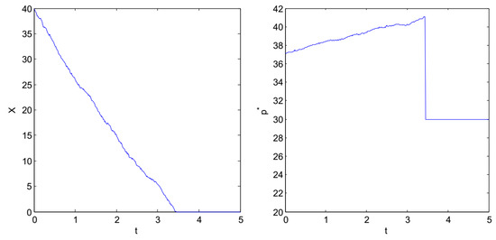
Figure 1. The evolution curves of the inventory level and the optimal selling price with time if $T<$ $t_d$.

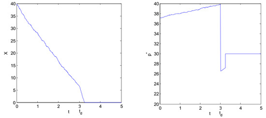
Figure 2. The evolution curves of the inventory level and the optimal selling price with time if $T>$ $t_d$.

In Figure 1, the sample path of stochastic process with $t_d=6$ and $T=5$ is simulated. In this case, shortages occur. It shows that the inventory level $X(t)$ decreases and is down to zero resulting from the demand before the deteriorating items occur. Meanwhile, the optimal selling price experiences increase due to the current inventory level when $X(t)>0$. After the stock is sold out, the $p^{*}(t,0)(=\overline{p})$ falls sharply and then maintains stable at 30 units until to the end of the cycle.

Then, another sample path of stochastic process with $t_d=3$ and $T=5$ is simulated based on the situation that shortages and deteriorations occur during a replenishment cycle, which is consistent with the realistic depiction of the retailer. The numerical simulation results are displayed in Figure 2. We can see that the inventory level $X(t)$ decreases with time under the optimal selling price owing to demand and deterioration. When deterioration occurs, a faster rate of decline can be observed. The optimal selling price raises to 40 units before the items deteriorate. It then drops sharply to 26 unit because of deterioration. The optimal selling price increases slightly again resulting from the reduction of inventory level. When the stock is sold out, the optimal selling price is elevated to 30 unit and kept constant until to the next replenishment cycle.

Moreover, the function of the evolution curve of the profit shown in Figure 3 is equal to

$$\begin{array}{c}\hfill {\int }_0^T(p^{*}(t,X(t))-c)(b+\alpha p^{*}(t,X(t)))dt-{\int }_0^{T}hX(t)dt-r{X}^2(T)\end{array}$$

when the remains occur and is equal to

$$\begin{array}{c}\hfill {\int }_0^{\tau }(p^{*}(t,X(t))-c)(b+\alpha p^{*}(t,X(t)))dt-{\int }_0^{\tau }hX(t)dt+{\int }_{\tau }^T(p^{*}(t,X(t))-c)(b+\alpha p^{*}(t,X(t)))e^{-\gamma (T-t)}dt\end{array}$$

when the shortages occur, where $\tau$ is the moment of the items sold out, and $X(t)$ is the current inventory level with the optimal selling price $p^{*}(t,X(t))$ and $X(0)=40$.

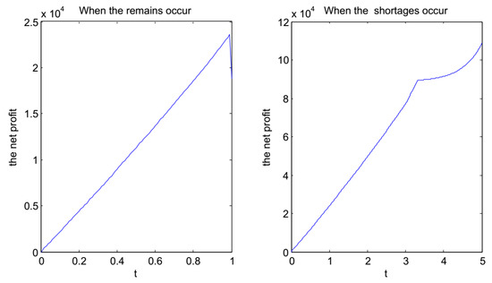
Figure 3. The evolution curves of the profit.

Figure 3 shows that when the remains occur, the expected total profit increases in $[0,1)$ and decreases at the end of replenishment cycle 1 resulting from the surplus cost. Besides, when the shortages occur, the expected total profit increases due to the partial backlogging, but its growth rate slows down, and the longer the waiting time, the smaller the growth rate.

Finally, we consider the evolution of the optimal selling price $p^{*}(0,x)$ and the optimal expected total profit $V(0,x;T)$ with respect to the inventory level x.

Example 2.

Consider the inventory system with the following parameters:

$$\begin{array}{c}b=50,\alpha =-1,\sigma =2,\theta =0.1,\hfill \\ C=20,c=10,r=1,h=2\hfill \\ \gamma =2,t_d=0.8.\hfill \end{array}$$

The optimal selling price $p^{*}(0,x)$ with respect to the inventory level under different values of $T=1,2,3$ is shown in Figure 4. It shows that the optimal selling price is decreasing with respect to the inventory level. Actually, the more the inventory level, the lower the optimal selling price. Besides, for the fixed inventory level x, prolonging the replenishment cycle will give rise to the increase of the optimal selling price.

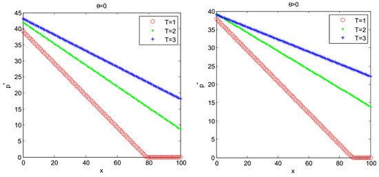
Figure 4. $p^{*}(0,x)$ with x about the different values of T.

The value function $V(0,x;T)$ with respect to the inventory level under different values of $T=1,2,3$ is displayed in Figure 5. It indicates that the optimal replenishment cycle is 3 and the optimal inventory level is 57 with the optimal selling price 20 almost.

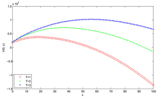
Figure 5. $V(0,x;T)$ with x about the different values of T.

5.2. Sensitivity Analysis

In this subsection, the influence of volatility of potential demand on the expected total profit is discussed via varying parameter $\sigma$ from 1 to 3 continuously.

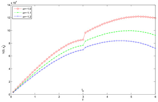
The optimal expected total profit is obtained with respect to $\sigma$ under the optimal selling price when other parameters are in accord with those in Example 1 as shown in Figure 6. The total expected profit for retailer will decrease with increase of the market potential uncertainty, indicating that a higher volatility of potential market demand will reduce the retailers’ profit. Therefore, the demand uncertainty of the marked should be fully considered when the manager makes plan for the future.

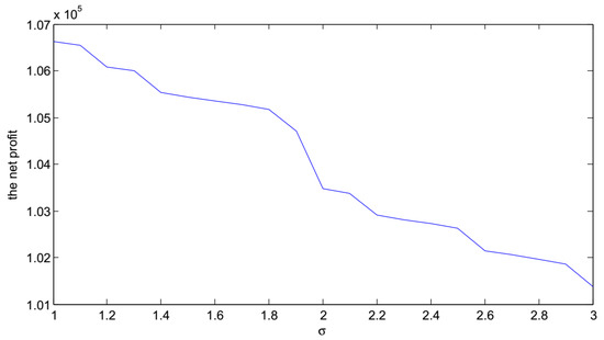
Figure 6. The expected total profit for different $\sigma$.

Then, we analyze the influences of changes in the system parameters on the optimal initial inventory level $X^{*}(0;T)$, the optimal selling price $p^{*}(0,X^{*}(0;T))$, the optimal replenishment cycle $T^{*}$, and the optimal expected total profit $V^{*}(0,X^{*}(0;T);T)$ according to Theorem 2. The model parameters are given as follows:

$$\begin{array}{c}b=50,\sigma =2,\theta =0.01,\gamma =2,\hfill \\ C=20,c=10,r=1,h=2,\hfill \\ S=100,t_d=3,\alpha =-1.1.\hfill \end{array}$$

Example 3.

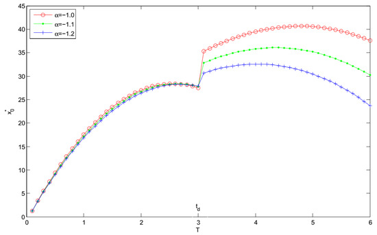
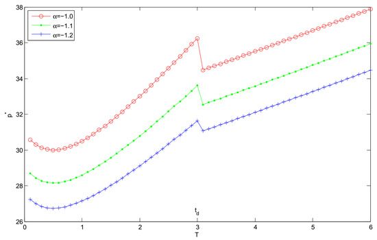
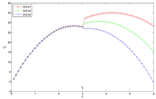
The optimal initial inventory level $X^{*}(0;T)$, the optimal selling price $p^{*}(0,X^{*}(0;T))$, and the optimal expected total profit $V^{*}(0,X^{*}(0;T);T)$ are obtained with respect to the optimal replenishment cycle $T^{*}$ about the different values of $\alpha =-1.0,-1.1,-1.2$ as shown in Table 1. Moreover, the curves of the above optimal results with respect to replenishment cycle are displayed in Figure 7, Figure 8 and Figure 9. On the basis of numerical results, the following inferences are made from the perspective of managers:

Table 1. The effects of $\alpha$ on $T^{*}$, $X^{*}(0;T^{*})$, $p^{*}(0,X^{*}(0;T^{*}))$, and $V^{*}(0,X^{*}(0;T^{*});T^{*})$.

$\mathit{\alpha }$	${\mathit{T}}^{*}$	${\mathit{X}}^{*}(0;{\mathit{T}}^{*})$	${\mathit{p}}^{*}(0,{\mathit{X}}^{*}(0;{\mathit{T}}^{*}))$	${\mathit{V}}^{*}(0,{\mathit{X}}^{*}(0;{\mathit{T}}^{*});{\mathit{T}}^{*})({10}^5)$
−1.0	5.3	40.1040	37.0381	1.2247
−1.1	5	35.1775	34.7441	0.9956
−1.2	4.6	31.8401	32.7993	0.8405

Figure 7. $X^{*}(0;T)$ with respect to T about the different values of $\alpha$.

Figure 8. $p^{*}(0,X^{*}(0;T))$ with respect to T about the different values of $\alpha$.

Figure 9. $V^{*}(0,X^{*}(0;T);T)$ with respect to T about the different values of $\alpha$.

• Figure 7, Figure 8 and Figure 9 show that $X^{*}(0;T)$, $p^{*}(0,X^{*}(0;T))$ and $V(0,X^{*}(0;T);T)$ increase with increase in the demand sensitivity to the selling price α for the fixed replenishment cycle length T. It indicates that when the selling price has a less impact on the demand, the retailer should raise selling price to achieve more profit.
• When the deteriorating items occur, the retailer should increase stock and lower the selling price to reduce the impact of the perishable items.
• When $\alpha =-1.2$, the retailer should keep less stocks, drop the selling price, and reduce the replenishment cycle after items deteriorate to achieve higher profit.
• When $\alpha =-1.0$, the retailer should keep more stocks, and raise the selling price after items deteriorate to maximize the profit.
• It can be seen that increasing the demand sensitivity to the selling price α will cause the increase of $T^{*}$ and $V^{*}(0,X^{*}(0;T^{*});T^{*})$. Furthermore, the optimal replenishment cycle and the optimal expected total profit are highly sensitive to the changes in the price sensitivity factor to the demand.

Example 4.

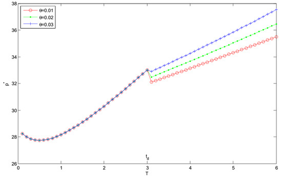
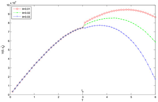
The optimal initial inventory level $X^{*}(0;T)$, the optimal selling price $p^{*}(0,X^{*}(0;T))$, and the optimal expected total profit $V^{*}(0,X^{*}(0;T);T)$ are obtained with respect to the optimal replenishment cycle $T^{*}$ about the different values of $\theta =0.01,0.02,0.03$ as shown in Table 2. The curves of the above optimal results with respect to replenishment cycle are given in Figure 10, Figure 11 and Figure 12. On the basis of numerical results, the following inferences are made from the perspective of managers:

Table 2. The effects of $\alpha$ on $T^{*}$, $X^{*}(0;T^{*})$, $p^{*}(0,X^{*}(0;T^{*}))$, and $V^{*}(0,X^{*}(0;T^{*});T^{*})$.

$\mathit{\alpha }$	${\mathit{T}}^{*}$	${\mathit{X}}^{*}(0;{\mathit{T}}^{*})$	${\mathit{p}}^{*}(0,{\mathit{X}}^{*}(0;{\mathit{T}}^{*}))$	${\mathit{V}}^{*}(0,{\mathit{X}}^{*}(0;{\mathit{T}}^{*});{\mathit{T}}^{*})({10}^5)$
0.01	4.9	34.1299	34.1856	9.4751
0.02	4.3	29.6720	33.0762	8.5439
0.03	3.7	26.3545	33.7969	7.7317

Figure 10. $X^{*}(0;T)$ with respect to T about the different values of $\theta$.

Figure 11. $p^{*}(0,X^{*}(0;T))$ with respect to T about the different values of $\theta$.

Figure 12. $V^{*}(0,X^{*}(0;T);T)$ with respect to T about the different values of $\theta$.

• For a fixed replenishment cycle length T, $X^{*}(0;T)$ and $V(0,X^{*}(0;T);T)$ increase whereas $p^{*}(0,X^{*}(0;T))$ decreases with the decreasing in the deterioration rate θ. The results show that a higher deterioration rate leads to a higher selling price, and a lower optimal initial inventory level and optimal expected total profit.
• When $\theta =0.01$, the retailer should keep more stocks and knock down selling price to get higher profit.
• When $\theta =0.03$, the retailer should keep less stocks, raise the selling price and reduce the replenishment cycle resulting from a higher deteriorating rate to maximize their profit.
• It can be found that $T^{*}$ and $V^{*}(0,X^{*}(0;T^{*});T^{*})$ decrease with the increasing in the deterioration rate θ. Moreover, the optimal replenishment cycle and the optimal expected total profit are highly sensitive to the change in the deterioration rate.

6. Conclusions

It is a major concern for retailers to manager non-instantaneous deteriorating items under an uncertain environment. In our work, a dynamic pricing and optimal control for a stochastic inventory system with non-instantaneous deteriorating items are considered. The demand is stochastic and governed by a diffusion process, and the demand rate is supposed to be a linear function of selling price. Besides, both shortages and surplus are allowed. The backlogging rate is variable and dependent on the waiting time for the next replenishment. Then, a stochastic optimal control model is established to maximize the expected total profit, and an exact expression of the optimal dynamic pricing is achieved through the dynamic programming principle. The solution shows the optimal selling price take the linear time-dependent feedback form of the current inventory level. Besides, it is worth noting that the inventory system we construct is stochastic, which can give a better description for actual situation, however, the optimal selling price is deterministic with respect to the current inventory level. According to those results, the managers can make pricing decision and adjust his strategy immediately to enjoy a maximum profit. Moreover, the optimal initial inventory level, the optimal selling price, the optimal replenishment cycle and the optimal expected total profit are obtained when the replenishment cycle starts at time 0. Finally, some numerical experiments are presented to demonstrate the developed model and the sensitivities analysis on major system parameters are carried out to provide some suggestions for managers.

Future study may pay attention to a stochastic production inventory system with non-instantaneous deteriorating items. Also, this work can be extended by considering the demand which is dependent on inventory level and selling price.

References

- Ghare, P.M.; Schrader, G.F. A model for exponentially decaying inventory. J. Ind. Eng. 1963, 14, 238–243. [Google Scholar]
- Covert, R.P.; Philip, G.C. An EOQ model for items with weibull distribution deterioration. AIIE Trans. 1973, 5, 323–326. [Google Scholar] [CrossRef]
- Shah, Y.K. An order-level lot-size inventory model for deteriorating items. AIIE Trans. 1977, 9, 108–112. [Google Scholar] [CrossRef]
- Goyal, S.K.; Giri, B.C. Recent trends in modeling of deteriorating inventory. Eur. J. Oper. Res. 2001, 134, 1–16. [Google Scholar] [CrossRef]
- Bakker, M.; Riezebos, J.; Teunter, R.H. Review of inventory systems with deterioration since 2001. Eur. J. Oper. Res. 2012, 221, 275–284. [Google Scholar] [CrossRef]
- Wu, K.S.; Ouyang, L.Y.; Yang, C.T. An optimal replenishment policy for non-instantaneous deteriorating items with stock-dependent demand and partial backlogging. Int. J. Prod. Econ. 2006, 101, 369–384. [Google Scholar] [CrossRef]
- Ouyang, L.Y.; Wu, K.S.; Yang, C.T. A study on an inventory model for non-instantaneous deteriorating items with permissible delay in payments. Comput. Ind. Eng. 2006, 51, 637–651. [Google Scholar] [CrossRef]
- Chang, J.H.; Lin, F.W. A partial backlogging inventory model for non-instantaneous deteriorating items with stock-dependent consumption rate under inflation. Yugosl. J. Oper. Res. 2010, 20, 35–54. [Google Scholar] [CrossRef]
- Whitin, T.M. Inventory Control and Price Theory. Manag. Sci. 1955, 2, 61–68. [Google Scholar] [CrossRef]
- Wee, H.M. A replenishment policy for items with a price-dependent demand and a varying rate of deterioration. Prod. Plan. Control. 1997, 8, 494–499. [Google Scholar] [CrossRef]
- Wu, K.S.; Ouyang, L.Y.; Yang, C.T. Coordinating replenishment and pricing policies for non-instantaneous deteriorating items with price-sensitive demand. Int. J. Syst. Sci. 2009, 40, 1273–1281. [Google Scholar] [CrossRef]
- Soni, H.N.; Patel, K.A. Joint pricing and replenishment policies for non-instantaneous deteriorating items with imprecise deterioration free time and credibility constraint. Comput. Ind. Eng. 2013, 66, 944–951. [Google Scholar] [CrossRef]
- Zhang, J.; Wang, Y.; Lu, L.; Tan, W. Optimal dynamic pricing and replenishment cycle for non-instantaneous deterioration items with inventory-level-dependent demand. Int. J. Prod. Econ. 2015, 170, 136–145. [Google Scholar] [CrossRef]
- Duan, Y.; Cao, Y.; Huo, J. Optimal pricing, production, and inventory for deteriorating items under demand uncertainty: The finite horizon case. Appl. Math. Model. 2018, 58, 331–348. [Google Scholar] [CrossRef]
- Li, Y.; Zhang, S.; Han, J. Dynamic pricing and periodic ordering for a stochastic inventory system with deteriorating items. Automatica 2017, 76, 200–213. [Google Scholar] [CrossRef]
- Geetha, K.V.; Udayakumar, R. Optimal lot sizing policy for non-instantaneous deteriorating items with price and advertisement dependent demand under partial backlogging. Int. J. Appl. Comput. Math. 2016, 2, 171–193. [Google Scholar] [CrossRef]
- Das, S.C.; Zidan, A.M.; Manna, A.K.; Shaikh, A.A.; Bhunia, A.K. An application of preservation technology in inventory control system with price dependent demand and partial backlogging. Alex. Eng. J. 2020. [Google Scholar] [CrossRef]
- Debata, S.; Acharya, M. An inventory control for non-instantaneous deteriorating items with non-zero lead time and partial backlogging under joint price and time dependent demand. Int. J. Appl. Comput. Math. 2017, 3, 1381–1393. [Google Scholar] [CrossRef]
- Agi, M.A.; Soni, H.N. Joint pricing and inventory decisions for perishable products with age-, stock-, and price-dependent demand rate. J. Oper. Res. Soc. 2020, 71, 85–99. [Google Scholar] [CrossRef]
- Chang, H.J.; Dye, C.Y. An EOQ model for deteriorating items with time varying demand and partial backlogging. J. Oper. Res. Soc. 1999, 50, 1176–1182. [Google Scholar] [CrossRef]
- Maihami, R.; Kamalabadi, I.N. Joint pricing and inventory control for non-instantaneous deteriorating items with partial backlogging and time and price dependent demand. Int. J. Prod. Econ. 2012, 136, 116–122. [Google Scholar] [CrossRef]
- Soni, H.; Suthar, D. Pricing and inventory decisions for non-instantaneous deteriorating items with price and promotional effort stochastic demand. J. Control Decis. 2018, 6, 1–25. [Google Scholar] [CrossRef]
- Abad, P.L. Optimal price and order size for a reseller under partial backordering. Comput. Ind. Eng. 2001, 28, 53–65. [Google Scholar] [CrossRef]
- Wang, S.P. An inventory replenishment policy for deteriorating items with shortages and partial backlogging. Comput. Oper. Res. 2002, 29, 2043–2051. [Google Scholar] [CrossRef]
- Dye, C.Y.; Ouyang, L.Y.; Hsieh, T.P. Inventory and pricing strategies for deteriorating items with shortages: A discounted cash flow approach. Comput. Ind. Eng. 2007, 52, 29–40. [Google Scholar] [CrossRef]
- Papachristos, S.; Skouri, K. An inventory model with deteriorating items, quantity discount, pricing and time-dependent partial backlogging. Int. J. Prod. Econ. 2003, 83, 247–256. [Google Scholar] [CrossRef]
- Farughi, H.; Khanlarzade, N.; Yegane, B.Y. Pricing and inventory control policy for non-instantaneous deteriorating items with time- and price-dependent demand and partial backlogging. Decis. Sci. Lett. 2014, 3, 325–334. [Google Scholar] [CrossRef][Green Version]
- Kogan, K.; Herbon, A. Inventory control over a short time horizon under unknown demand distribution. IEEE Trans. Automat. Contr. 2016, 61, 3058–3063. [Google Scholar] [CrossRef]
- Zwillinger, D. Handbook of Differential Equations; Academic Press: New York, NY, USA, 1989. [Google Scholar]
© 2020 by the authors. Licensee MDPI, Basel, Switzerland. This article is an open access article distributed under the terms and conditions of the Creative Commons Attribution (CC BY) license (http://creativecommons.org/licenses/by/4.0/).