A Stochastic Kinetic Type Reactions Model for COVID-19

Abstract

We propose two stochastic models for the Coronavirus pandemic. The statistical properties of the models, in particular the correlation functions and the probability density functions, were duly computed. Our models take into account the adoption of lockdown measures as well as the crucial role of hospitals and health care institutes. To accomplish this work we adopt a kinetic-type reaction approach where the modelling of the lockdown measures is obtained by introducing a new mathematical basis and the intensity of the stochastic noise is derived by statistical mechanics. We analysed two scenarios: the stochastic $SIS$-model (Susceptible ⇒ Infectious ⇒ Susceptible) and the stochastic $SIS$-model integrated with the action of the hospitals; both models take into account the lockdown measures. We show that, for the case of the stochastic SIS-model, once the lockdown measures are removed, the Coronavirus infection will start growing again. However, the combined contributions of lockdown measures with the action of hospitals and health institutes is able to contain and even to dampen the spread of the SARS-CoV-2 epidemic. This result may be used during a period of time when the massive distribution of vaccines in a given population is not yet feasible. We analysed data for USA and France. In the case of USA, we analysed the following situations: USA is subjected to the first wave of infection by Coronavirus and USA is in the second wave of SARS-CoV-2 infection. The agreement between theoretical predictions and real data confirms the validity of our approach.

1. Introduction

The current number of infectious people with SARS-CoV-2 brought us back to the lockdown phase, but tracking and swabs give a clearer vision of the situation. By reading the figures on new cases of positivity, it seems that we are returning back to mid-April 2020. Hospitalisations are also growing, including new hospitalisations in intensive care units. In this context, the situation appears very different compared to the first months of the epidemic, when the prolonged lockdown was necessary, which allowed reduction in the spread of the Coronavirus in a significant way. The percentage ratio between new cases and swabs now stands at around 5% [1]. It is therefore from 30 percent of the “darkest” periods of the pandemic in certain European Countries. However, these data tend to increase further preventive strategies, focusing on tracing and beyond, taking into account that in some countries the “weight” of the pandemic is starting to be felt again on hospitals. So, we are in the middle of the second wave, but the virus circulates among humans and therefore the lockdown period has limited its spread, so much so that we reached a sort of “stagnation” in the months of June and July with a subsequent resumption in August. However, the virus did not change and the clinical manifestations that it induces have not changed [2]. In this second period of COVID-19, we may trust statistical data much more thanks to the increased number of swabs done and the tracing and monitoring of people who have contracted the SARS-CoV-2 infection. Of course, there are still some cases, especially for asymptomatic subjects who unfortunately can transmit the infection: about 20% of cases of contagion can in fact be attributed to subjects who do not show any health problems. This situation also explains why the percentage of positive swabs in the first weeks of the lockdown was around 30 percent, while today it is much lower. Anyway, we are still far from the figures of several thousand of last March-April, but the trend is still on the rise. For this reason, it is essential also to hold the infections through “ad hoc” measures (lockdown, quarantine, isolation). The carelessness during the summer holidays has created a clear epidemiological link, as the number of cases started to rise again in August and now we have to face the situation, also because there are signs from nearby France warning of this problem.

• USA situation. After sustained declines in the number of COVID-19 cases over recent months, restrictions are starting to ease across the United States. The numbers of new cases are either falling or stable at low numbers in some states, but they are surging in many others. Overall, the USA is experiencing a sharp increase in the number of new cases per day and, by late June, had surpassed the peak rate of the spread in early April. In the USA, cases are rising quickly right now. With more than 11 million confirmed cases, the USA has the highest number of infections in the world and the spread of the Coronavirus shows no sign of slowing down. During the spring wave, swabs were mostly limited to confirming cases in people who were already in hospitals, meaning the true scale of that outbreak was not fully captured. However the latest data compiled by the COVID Tracking Project shows the current surge is not just down to increased testing; the number of tests carried out in USA was up by 12.5% week on week, while the number of cases increased by more than 40% [3]. One likely cause is the change of season and colder weather driving people indoors to socialise, where the risk of spread is heightened due to less social distancing and poor ventilation. The strain on hospitals is growing. Because of the change in the level of testing, a better way to compare waves is to look at the number of people being admitted to hospitals because of COVID-19. These data show that roughly the same number of people across the USA were in hospital during the first and second waves of the outbreak. However, there are already more people in hospitals during the current wave—more than 70,000 at the moment. New deaths per day have not begun to climb, but some hospitals’ intensive care units have recently reached full capacity [4]. This wave is hitting every USA region. We can say that the USA as a whole is not in a second wave because the first wave never really stopped. The virus is simply into new populations or is resurgent in places that let down their guard too soon. This time around, every region is seeing a spike in new cases [3].

• France situation. Coronavirus cases in France rose dramatically, but the number of daily deaths declined. The total number of infections stands at around of 1,829,659, with the death toll standing at 42,207, according to the Ministry of Health. The overall downward trend is a positive sign after Coronavirus numbers increased drastically by reaching a peak of 86,852 cases. Some 99 departments throughout France remain in a vulnerable position with 3042 clusters of infection considered serious [5]. France now has the fourth highest number of infections in the world behind the USA, India and Brazil. Despite the French government’s efforts to slow down the spread of the virus with targeted measures such as lockdown and isolation, the rate of infections has continued to rise across the country. Talks regarding the occurrence of a second wave, and how to avoid it, has been around since the end of the spring lockdown, but the current situation seems to suggest it was unavoidable. One month after the lockdown measures were applied in major cities starting in Paris, and three weeks after extending it to almost the whole country, France can see the light at the end of the dark tunnel of the second wave of Coronavirus. The French Health Minister announced that he believes that the peak of the pandemic has passed, and control has been regained. Indeed, looking at the data, after a peak of 86,000 cases as recorded on November 7, the country has moved on to figures of around 30,000 daily infections with a minimum level of 23,000 as recorded on November 13. Figures are returning in line with those of a month ago when the lockdown began [6]. However, the country will remain in a second nationwide lockdown whicch will continue until Dec. 1 unless the number of infections and deaths decrease in a significant way.

• Modelling the spread of SARS-CoV-2 infection. Until the vaccine arrives, the tried-and-true public health measures taken on the last months (social distancing, universal mask wearing, frequent hand-washing and avoiding crowded indoor spaces) are the ways to stop the first wave and thwart a second one. In addition, when there are surges such as those happening now in the world, further reopening plans need to be put on hold. Meanwhile, in order to understand the situation, theoretical studies, mainly based on mathematical models with the use of up-to-date data, must be carried on in order to understand the of this pandemic in the future as well as to provide predictions. In this study, we propose a simple stochastic model with the objective to show how public health interventions can influence the outcome of the epidemic, by limiting and even dampening the of the SARS-CoV-2 epidemic, while waiting for the production and delivery of an effective vaccine. The analysis is performed by assigning the population to different compartments with labels, such as S, I, R and D (Susceptible, Infectious, Recovered, and Deaths). People can move between the compartments. The order of labels shows the flow patterns between compartments; for example $SIS$ means susceptible, infectious and, therefore, Susceptible again. The origin of these models is at the beginning of the twentieth century [7]. The goal of our model is to predict how a disease spreads, or the dynamics of the number of infectious people, as well as the duration of the COVID-19 pandemic. The dynamics of this kind of models is governed by ordinary differential equations (O.D.E.s). Generally, these O.D.E.s are deterministic (see, for example, [8,9,10,11,12]).

In this work the dynamics is governed by stochastic differential equations, which describe reality in a more realistic way. We would like to stress that testing, e.g., swabs, may provoke fluctuations in experimental data, but these kinds of fluctuations are not quoted in the current work. The stochasticity dealt with in this manuscript concerns the dynamics of intrinsic fluctuations which arise spontaneously in a macroscopic system, and which satisfy the laws of statistical mechanics [13]. The main objective of our series of studies is to obtain the correct space-time stochastic differential equations which could describe realistic situations of spread of SARS-CoV2 pandemic in large countries. This goal can only be achieved if we are able to

(1) Model the distribution of hospitals and health institutes in a country;

(2) Model the distribution of the poles of attraction of susceptible people (e.g., shopping centers, workplaces, etc.);

(3) Identify a mechanism able to establish when a pole of attraction is “saturated” with infected people, by proposing alternative poles of attraction;

(4) Modelling the Lockdown and Quarantine measures adopted by the Government of a particular country;

(5) Describe the dynamics of intrinsic (i.e., spontaneous) fluctuations to which a macroscopic system is subjected by methods of statistical mechanics.

At first glance, such a working program would appear to be too ambitious and, to our knowledge, the state-of-the-art of current alternative techniques are unable to resolve the issues listed above. The Kinetic-Type Reaction (KTR) approach proposed by us is very promising and allows to achieve this goal in a relatively simple way. Indeed the kinetic-type reaction approach

(a) Models each actor by a dedicated chemical species that can only be created or destroyed as the result of one, or several, elementary steps;

(b) Allows to determine the dynamics of the system starting from elementary steps;

(c) Thanks to its flexibility, allows to analyse complex situations when several variables are involved, such as R, Q, $R_h$, $I_h$ etc.

We anticipate that, by adding extra space-time dependent contributions, inspired by a biological analogy, to the deterministic dynamic equations obtained by applying the KTR model, we have been able to determine the correct space-time stochastic partial differential equations which are suitable to describe the spread of SARS-CoV2 infection not only in single regions, but also in space extended countries. A work and related interactive simulations, where predetermined distributions of poles of attraction are set up, is in progress. In our view, this is the novelty of our approach with respect to models currently proposed in the literature. To the best of the authors’ knowledge, our approach has never been proposed before.

The paper is organised as follows. In Section 2, we study the deterministic $SIS$-model in presence of the lockdown measures. We shall see that as soon as the lockdown measures are stopped, the of Coronavirus begins to grow back vigorously once a certain threshold is exceeded. In Section 2.1, we ask ourselves the following question: Let us suppose a situation in which a government needs a number x of weeks (e.g., 6 weeks) before being able to deliver an effective vaccine. What is the minimum expected value of infectious people that should be seen, after the adoption of severe lockdown measures imposed on the population, in order to be sure that after x-weeks (e.g., after 6 weeks) the total number of infectious individuals by Coronavirus remains below a threshold pre-set in advance, and acceptable from a medical and political point of view? Section 2.1 answers the above-mentioned question for the $SIS$-model subjected to lockdown measures. In Section 3, we introduce, and study, the Stochastic $SIS$-model subjected to lockdown measures (the ${\left(SIS\right)}_L$-model). We compute the relevant correlation functions as well as the probability density function. Hospitals and health institutes play a crucial role in hindering the of Coronavirus. In Section 4, we propose a model that accounts for people who are only traced back to hospitalised infectious individuals. This model is referred to as the ${\left(SIS{I}_h{r}_h{d}_h\right)}_L$-model. We shall see that beyond a certain threshold of hospital capacities, the coronavirus is not only kept under control, but its tends to diminish in time. Therefore, the combined effect of lockdown measures with ef = ficient hospitals and health measures are able to contain and even dampen the spread of the SARS-CoV-2 epidemic, while waiting for the delivery of a limited number of vaccines in a given population. In Section 5, we study the simplified ${\left(SIS{I}_h\right)}_L$ stochastic model by computing the relevant correlation functions.

This approach is in line with the procedure normally adopted by the scientific community. When a process is complex, it is customary to start by analysing the simplest model, the SI(R)S model in this case, subjected to lockdown measures and perturbed by white noise. Of course, the role of the lockdown measures is not to shorten the infectious period of an infected individual, but rather to intervene on susceptible people. The noise takes into account the intrinsic fluctuations of the infected individuals, which are governed by the laws of statistical mechanics. These tasks have been accomplished by adopting a kinetic-type reactions approach, where the compartments S, I, and R are seen as “chemically active molecules” (see Section 2), and by showing two theoretical results which we report for the first time in the literature, namely:

(1) The lockdown measures (also applicable to the quarantine and isolation measures) are modelled by introducing a new (complete) mathematical base of functions (see Equation (12));

(2) The intensity of the white noise is derived by the laws of statistical mechanics (see Equation (A11)).

Comparison between theoretical predictions and real data for USA and France can be found in Section 6. Concluding remarks are reported in Section 7. The derivation of the exact solution of Richards equation in presence of the restriction measures as well as an estimation of the intensity of the noise by Statistical Mechanics methods can be found in the Appendices Appendix A and Appendix B.

2. The Deterministic Model in Presence of the Lockdown Measures-the (SIS)_L-Model

The current work starts from the following hypothesis commonly supported by the most accredited virologists: the SARS-CoV-2 behaves like other viruses which cause respiratory diseases (see, for instance, ref. [14]). The common cold and influenza, do not give any long-lasting immunity. Such infections do not give immunity upon recovery from infection, and individuals become susceptible again. Hence, according to the above-cited hypothesis we propose the following simplest compartmental model:

$$S+I\stackrel{\mu }{\to }2I$$

(1)

In our model the SARS-CoV-2 infection does not leave any immunity, thus individuals, after recovery, return back into the S compartment. This added detail can be seen by including an R class in the middle of the model

$$\begin{array}{c}S+I\stackrel{\mu }{\to }2I\hfill \\ I\stackrel{\gamma }{\to }R\stackrel{{\gamma }_1}{\to }S\hfill \end{array}$$

(2)

In this work, Equation (2) has to be interpreted as follows. The entire process is described by adopting a kinetic-type reactions approach where the lockdown measures are modelled by some kind of inhibitor reactions where susceptible individuals can be trapped into inactive states. In addition, the substrate is associated to the infected people and the product to the recovered people, respectively. From Equation (2), we get the following O.D.E.s for S, R, and I:

$$\begin{array}{c}\frac{dS}{dt}=-\sigma \frac{S}{N_{Tot.}}I+{\gamma }_{1}R\hfill \\ \frac{dI}{dt}=\sigma \frac{S}{N_{Tot.}}I-\gamma I\hfill \\ \frac{dR}{dt}=\gamma I-{\gamma }_{1}R\hfill \end{array}$$

(3)

with $N_{Tot.}$ denoting the total population and $\sigma \equiv \mu N_{Tot.}$. By assuming that the dynamics of R is much faster that those of S and I, we may set $dR/dt\simeq 0$ and system (3) reduces to

$$\begin{array}{c}\frac{dS}{dt}\simeq -\sigma \frac{S}{N_{Tot.}}I+\gamma I\hfill \\ \frac{dI}{dt}=\sigma \frac{S}{N_{Tot.}}I-\gamma I\hfill \end{array}$$

(4)

which corresponds to the model

$$\begin{array}{c}S+I\stackrel{\mu }{\to }2I\hfill \\ I\stackrel{\gamma }{\to }S\hfill \end{array}$$

(5)

In the relevant literature, model (5) is referred to as the $SIS$-model (see, for example, [15]). Notice that condition $dR/dt\simeq 0$ was adopted only for simplicity. This allows to obtain relevant results by performing calculations analytically, without having to solve numerically system (3). From Equation (4) we get the conservation law

$$\frac{dS}{dt}+\frac{dI}{dt}=0\mathrm{or}S+I=N_{Tot.}$$

(6)

Hence, the dynamics of infectious people is governed by the logistic model

$$\frac{dI}{dt}=(\sigma -\gamma )I\left(1-\frac{\sigma }{N_{Tot.}(\sigma -\gamma )}I\right)$$

(7)

or

$$\begin{array}{c}\frac{dI}{dt}=\tilde{\alpha }I\left(1-\frac{I}{K}\right)\mathrm{with}\hfill \\ \tilde{\alpha }\equiv \sigma \left(1-\frac{\gamma }{\sigma }\right);K\equiv N_{Tot.}\left(1-\frac{\gamma }{\sigma }\right)\hfill \end{array}$$

(8)

where $\tilde{\alpha }$ and K denote the linear growing rate of the COVID-19 and the carrying capacity, respectively.

Lockdown measures are mainly based on an isolation of susceptible individuals, eventually with removal of infected people by hospitalisation. In our model, the effect of lockdown measures are taken into account by introducing in the $SIS$-model the lockdown-induced decrease rate $c\left(t\right)$

$$\begin{array}{c}S+I\stackrel{\mu }{\to }2I\hfill \\ I\stackrel{\gamma +c\left(t\right)}{\to }S\hfill \end{array}$$

(9)

where

$$\begin{array}{c}c\left(t_L\right)=0\mathrm{for}t=t_L\hfill \\ c\left(t\right)>0\mathrm{for}t>t_L\hfill \end{array}$$

(10)

in which $t_L$ denotes the time when the lockdown measures are applied. The meaning of kinetic reactions (9) is the following. Clearly, lockdown measures act on the susceptible individuals but they are unable to affect the chemical capacity (i.e., to decrease the infection capacity) of the Coronavirus. Hence, the value of the kinetic reaction $\mu$ must remain constant and the final effect of these lockdown measures is to increase the number of susceptible people “at the expense” of infected people (since $S+I=const.$). According to the model, this can be done only by increasing the value of the kinetic constant $\gamma$. Note that if the effect of the block were to decrease the value of the kinetic constant $\mu$, we would get the non-sense result that the carrying capacity of infected persons would increase over time. Finally, the corresponding deterministic differential equations for the COVID-19 model in presence of the lockdown measures reads then:

$$\begin{array}{c}\frac{dS}{dt}=-\sigma \frac{S}{N_{Tot.}}I+\gamma I+c\left(t\right)I\hfill \\ \frac{dI}{dt}=\sigma \frac{S}{N_{Tot.}}I-\gamma I-c\left(t\right)I\hfill \end{array}$$

(11)

Equation (9) may be referred to as the ${\left(SIS\right)}_L$-model where L stands for $Lockdown$. The general expression for the lockdown-contribution, $c\left(t\right)$, may be obtained as follow.

(1) At $t=t_L$, $c\left(t_L\right)=0$. This corresponds to the requirement that the lockdown measures start at time $t=t_L$;

(2) $c\left(t\right)$ must always be a positive function for all $t>t_L$ and for all kind of scenarios;

(3) for all $t>t_L$ and for all kind of scenarios, $c\left(t\right)$ must be a function able to bend, downwardly, the trend of the curve of infected people.

After that, we may proceed as usual. We look for a class of functions satisfying the above three requirements under the form of polynomials (or fractions of polynomials) by bearing in mind that the degrees of the polynomials must be chosen in such a way that the curve of infected people can be bent downwards. This requirement must be satisfied by each term of the series.

(4) Ultimately, we have to prove that the obtained series constitutes a complete base of functions. Here, we shall not discuss on the completeness of the basis functions ${\{{\widehat{t}}^{i+1}-{\widehat{t}}^{-j}\}}_{i,j=0,1,\dots }$. This will be subject of a future work.

Finally, the general expression for the lockdown measures, $c\left(t\right)$, may be cast into the form

$$c(\widehat{t})=\sum _{i,j=0}^{\infty }{\beta }_{ij}\left({\widehat{t}}^{i+1}-{\widehat{t}}^{-j}\right)\mathrm{for}\widehat{t}\ge 1$$

(12)

with $\widehat{t}$ denoting the normalised time $\widehat{t}\equiv t/t_L$ and ${\beta }_{ij}$ are real numbers. Note that, the above conditions (2) and (3) impose strict restrictions on the coefficients ${\beta }_{ij}$. Now, we look for a lockdown expression which takes into account only the most relevant terms. The first two terms of the series (12) are

$$c(\widehat{t})\simeq {\beta }_{00}(\widehat{t}-1)+{\beta }_{01}\left(\frac{{\widehat{t}}^2-1}{\widehat{t}}\right)\mathrm{with}\widehat{t}\ge 1$$

(13)

In References [16,17,18] we can find a huge amount of fittings of experimental data carried out for different countries and several SARS-diseases. The results of the fittings have shown that the most relevant contribution is expressed by the term $(t^2-t_L^2/t)$ while the term $(t-t_L)$ provides an irrelevant contribution in comparison with the previous one. Of course, there are situations where the term $(t-t_L)$ turns out to be significant, e.g., in chemotherapy that starts with a log-kill effect. In this case, c(t) is the therapy-induced death rate, modelled by the term $(t-t_C)$ since it is imposed at the beginning, and finely calibrated, from the outside. Finally, in our case we get

$$c(\widehat{t})\simeq \beta \left(\frac{{\widehat{t}}^2-1}{\widehat{t}}\right)\mathrm{with}\beta >0\mathrm{and}\widehat{t}\ge 1$$

(14)

with $\beta \equiv {\beta }_{01}=const.$ denoting the intensity of the lockdown measures. Equation (14) is the expression for the lockdown measures which will be considered in this work. Notice that Equation (14) generalises the lockdown term introduced in Reference [16]. By taking into account Equation (6), the deterministic differential equation for the infectious people, in presence of lockdown measures, reads

$$\frac{dI}{d\widehat{t}}=\alpha I\left(1-\frac{I}{K}\right)-\beta \left(\frac{{\widehat{t}}^2-1}{\widehat{t}}\right)I$$

(15)

with $\alpha \equiv \tilde{\alpha }{t}_L$. As shown in the Appendix A, the exact solution of Equation (15) reads

$$I=\frac{A{\widehat{t}}^{\beta }exp(-{(\widehat{t}-\alpha /\beta )}^2/\sigma )}{1+A\alpha /K{\int }_1^{\widehat{t}}{x}^{\beta }exp(-{(x-\alpha /\beta )}^2/\sigma )dx}$$

(16)

where $\sigma \equiv 2/\beta$. Equation (16) can be rewritten into the form

$$I=\frac{I_0{\widehat{t}}^{\beta }exp({(1-\alpha /\beta )}^2/\sigma )exp(-{(\widehat{t}-\alpha /\beta )}^2/\sigma )}{1+(I_0\alpha /K)exp({(1-\alpha /\beta )}^2/\sigma ){\int }_1^{\widehat{t}}{x}^{\beta }exp(-{(x-\alpha /\beta )}^2/\sigma )dx}$$

(17)

with $I_0$ denoting the value of the total cases at the time when the lockdown measures are applied, i.e., $I_{\widehat{t}=1}=I_0$. Notice that for large values of the carrying capacity, Equation (17) has the limiting behaviour

$$I\simeq I_0{\widehat{t}}^{\beta }exp({(1-\alpha /\beta )}^2/\sigma )exp(-{(\widehat{t}-\alpha /\beta )}^2/\sigma )$$

(18)

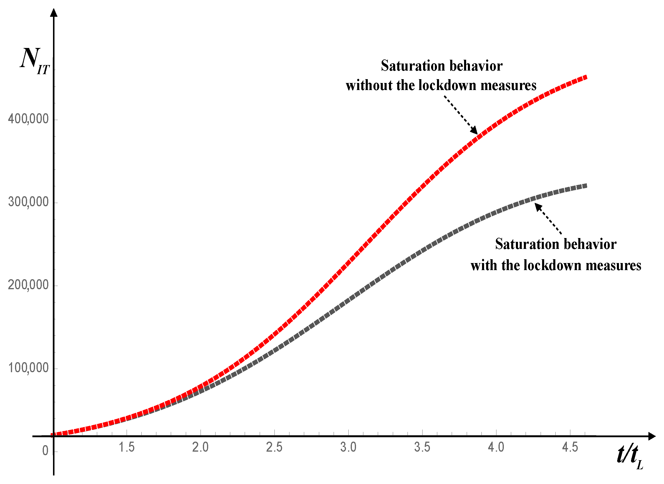
Figure 1 shows two solutions of model (15) for Italy, during the first wave of infection by SARS-CoV-2. The red dotted line refers to the solution without the lockdown measures and the dark dotted line to the solution when the lockdown measures were applied.

2.1. The Second Wave of COVID-19 Pandemic in the ${\left(SIS\right)}_L$-Model

The basic reproduction number, $R_0$, is defined as the expected number of secondary cases produced by a single (typical) infection in a completely susceptible population. An epidemic occurs if the number of infected individuals increases, i.e., $dI/dt>0$

$$\sigma \frac{S}{N_{Tot.}}I-\gamma I>0\mathrm{or}\frac{\sigma }{\gamma }\frac{S}{N_{Tot.}}>1$$

(19)

In this case, $R_0=\sigma /\gamma$. When lockdown measures are interrupted, the dynamics of the process is governed again by Equation (8). For Italy, in the first wave we have $R_0>1$, so $K>0$. From Equation (8) we get

$$\frac{\sigma }{\gamma }>1\mathrm{hence}\alpha >0\mathrm{and}\underset{\widehat{t}\to \infty }{lim}I=K$$

(20)

The above relations mean, from a biological perspective, that the disease will remain permanently endemic into the population. Notice that the inflection point of the logistic curve (8) occurs at time $t=t_f$ with

$${\widehat{t}}_f=\frac{1}{\alpha }log\left(\frac{K}{I_L}-1\right)$$

(21)

with $I_L$ denoting the number of infectious people when the lockdown measures start to be applied. It is easily checked that the inflection point, $P_f$, has coordinates $P_f=({\widehat{t}}_f,I_f=K/2)$. In our forthcoming reasoning, we shall see that the inflection point plays an important role in our analysis [19]. To summarise, after removing the lockdown measurements, say at time ${\widehat{t}}_1$, the number of infectious people will start to rise again from the value $I_1$, with $I_1\equiv I_{t={\widehat{t}}_1}$, following again a growth rate given by the logistic curve (8). This new growth of outbreak is referred to as the second wave of COVID-19. Now, our goal is to answer the following question: “Given a fixed value of infectious people, say $\tilde{I}$, determine the minimum value that $I_1$ should have so that the number of infectious people is less than $\widehat{I}$, during an entire period from ${\widehat{t}}_1$ to ${\widehat{t}}_f$”. We note that within the interval ${\widehat{t}}_1\le \widehat{t}\le {\widehat{t}}_f$ the number of infectious people grows quite slowly. Let us decide to interrupt the lockdown measures at time ${\widehat{t}}_2$. Hence, during the time interval $\Delta \widehat{t}={\widehat{t}}_2-{\widehat{t}}_1$, the population will no longer be subjected to lockdown measures. To answer the above-mentioned question, firstly we have to determine the range-values of $I_1$ such that $I_1<I_f=K/2$ for all $\widehat{t}\in \Delta \widehat{t}$, with $\Delta \widehat{t}<{\widehat{t}}_f-{\widehat{t}}_1$. It is easily checked that $I_1$ should satisfy the condition

$$0\le I_1<\frac{K}{1+exp(\alpha \Delta \widehat{t})}$$

(22)

Now, we have to require that after a lapse of time $\Delta \widehat{t}$, the number of infectious individuals must be lower than a fixed a priori value $\tilde{I}$, with $\tilde{I}<K/2$. The result is easily obtained by writing the initial condition as

$$I_1=\frac{K}{1+exp(\alpha \Delta \widehat{t})}-Kx\mathrm{with}0<x\le \frac{1}{1+exp(\alpha \Delta \widehat{t})}$$

(23)

and by determining the range of values of x such that the inequality

$$\frac{K}{1+(K/I_1-1)exp(-\alpha \Delta \widehat{t})}\le \tilde{I}<\frac{K}{2}$$

(24)

is satisfied. After a little algebra, we get

$$0\le I_1\le \tilde{I}\frac{2+exp\alpha \Delta \widehat{t}+exp(-\alpha \Delta \widehat{t})}{(1+exp(\alpha \Delta \widehat{t}))(\tilde{I}/K(exp(\alpha \Delta \widehat{t}))+exp(-\alpha \Delta \widehat{t})+1+exp(\alpha \Delta \widehat{t}))}$$

(25)

To summarise, if the lockdown measures are interrupted at time ${\widehat{t}}_1$, during the successive period of time $\Delta \widehat{t}={\widehat{t}}_2-{\widehat{t}}_1$ the number of infectious remains inferior to a preset number $\tilde{I}$ if the number of the infectious at the end of the lockdown measures is inferior to $I_1$, with $I_1$ given by the r.h.s. of Equation (25). A schematic representation of the second wave of SARS-CoV-2 infection is shown in Figure 2.

As an example, let us consider the case of the Italian situation. Figure 3 shows $I_1$ versus $\tilde{I}$ and $\Delta \widehat{t}$ such that 50,000 $\le \tilde{I}\le K_{IT}$.

As shown in Figure 4, if we set the value $\tilde{I}=$ 50,000, the maximum value of $I_1$ is $I_1\simeq 9500$ for $t\simeq t_L$, and $I_1\simeq 700$ for $t\simeq 2t_L$, respectively.

3. The Stochastic (SIS)_L-Model

The Stochastic version of Equation (15) reads

$$\frac{dI}{d\widehat{t}}=\alpha I\left(1-\frac{I}{K}\right)-\beta \left(\frac{{\widehat{t}}^2-1}{\widehat{t}}\right)I+\xi (\widehat{t})$$

(26)

with $\xi (\widehat{t})$ denoting a white noise

$$\begin{array}{c}<\xi (\widehat{t})>=0\hfill \\ <\xi (\widehat{t})\xi ({\widehat{t}}^{\prime })>=\eta \delta (\widehat{t}-{\widehat{t}}^{\prime })\hfill \end{array}$$

(27)

and $\sqrt{\eta }$ is the intensity of the noise. $\delta$ denotes the Dirac delta function (distribution). Let us now consider the system at the reference state $I_{RS}$, which is the solution of the deterministic equation

$$\frac{d{I}_{RS}}{d\widehat{t}}=\alpha I_{RS}\left(1-\frac{I_{RS}}{K}\right)-\beta \left(\frac{{\widehat{t}}^2-1}{\widehat{t}}\right)I_{RS}$$

(28)

subjected to a perturbation of small amplitude $\delta I$, i.e.,

$$I(\widehat{t})=I_{RS}(\widehat{t})+\delta I(\widehat{t})$$

(29)

Our goal is to compute the relevant statistical correlation functions of this processes, i.e., $<\delta I(\widehat{t})\xi (\widehat{t})>$ and $<\delta I(\widehat{t})\delta I({\widehat{t}}^{\prime })>$. Our task can easily be accomplished by recalling the following theorem (see, for example, [20,21,22,23]):

For a system of Langevin equations describing the temporal evolution of the processes $(x_1,\dots ,x_n)$:

$$\begin{array}{c}\frac{d{x}_i}{dt}=f_i(x_1,\dots ,x_n)+{\xi }_i\left(t\right)i=1,\dots ,n\hfill \\ <{\xi }_i\left(t\right)>=0;<{\xi }_i\left(t\right){\xi }_j\left(t^{\prime }\right)>={\eta }_{ij}\delta (t-t^{\prime })\hfill \end{array}$$

(30)

the following equations are valid:

$$\begin{array}{c}<x_i\left(t\right){\xi }_j\left(t^{\prime }\right)>=0\mathrm{if}{t}^{\prime }>t\hfill \\ <x_i\left(t\right){\xi }_j\left(t\right)>=\frac{1}{2}{\eta }_{ij}\hfill \end{array}$$

(31)

Now, we assume that the perturbation $\delta I$ is of order $\sqrt{\eta }$ (with $\sqrt{\eta }$ considered as a small parameter) and we expand Equation (26) up to the first order in $\sqrt{\eta }$. We get

$$\begin{array}{c}\frac{d{I}_{RS}(\widehat{t})}{d\widehat{t}}=\alpha I_{RS}(\widehat{t})\left(1-\frac{I_{RS}(\widehat{t})}{K}\right)-\beta \left(\frac{{\widehat{t}}^2-1}{\widehat{t}}\right)I_{RS}(\widehat{t})\left(\mathrm{at}\mathrm{the}\mathrm{zero}\mathrm{order}\right)\hfill \\ \frac{d}{d\widehat{t}}\delta I(\widehat{t})=\left(\alpha -\frac{2\alpha }{K}{I}_{RS}(\widehat{t})-\beta \frac{{\widehat{t}}^2-1}{\widehat{t}}\right)\delta I(\widehat{t})+\xi (\widehat{t})\left(\mathrm{at}\mathrm{the}\mathrm{first}\mathrm{order}\right)\hfill \end{array}$$

(32)

Solution $I_{RS}(\widehat{t})$ is given by Equation (17) and the exact solution for $\delta I(\widehat{t})$ is easily obtained:

$$\begin{array}{cc}\hfill I_{RS}(\widehat{t})=& \frac{I_{0RS}{\widehat{t}}^{\beta }exp({(1-\alpha /\beta )}^2/\sigma )exp(-{(\widehat{t}-\alpha /\beta )}^2/\sigma )}{1+(I_{0RS}\alpha /K)exp({(1-\alpha /\beta )}^2/\sigma ){\int }_1^{\widehat{t}}{x}^{\beta }exp(-{(x-\alpha /\beta )}^2/\sigma )dx}\hfill \\ \hfill \delta I(\widehat{t})=& t^{\beta }exp\left(\alpha (\widehat{t}-1)-1/2\beta ({\widehat{t}}^2-1)-2\alpha G(\widehat{t})/K\right)(\delta I\left(1\right)\hfill \\ \hfill & +{\int }_1^{\widehat{t}}dx\xi \left(x\right)\left(x^{-\beta }exp(-\alpha (x-1)+1/2\beta (x^2-1)+2\alpha G\left(x\right)/K)\right))\hfill \\ \hfill & \mathrm{with}G(\widehat{t})\equiv {\int }_1^{\widehat{t}}{I}_{RS}\left(x\right)dx\hfill \end{array}$$

(33)

Solution (33) allows to check the validity of Equation (31). Indeed, the correlation function $\delta I\left(t\right)$-noise at the same time reads

$$<\delta I(\widehat{t})\xi (\widehat{t})>=\frac{\eta }{2}$$

(34)

where Equation (30) and the properties of Dirac’s delta function have been taken into account. The equation for the second moment $<\delta I^2(\widehat{t})>$ is easily obtained by multiplying both sides of the second equation of system (32) by $2\delta I\left(t\right)$ and by taking into account Equation (31). We get

$$\frac{d}{d\widehat{t}}<{(\delta I(\widehat{t}))}^2>=2\left(\alpha -\frac{2\alpha }{K}{I}_{RS}(\widehat{t})-\beta \frac{{\widehat{t}}^2-1}{\widehat{t}}\right)<{(\delta I(\widehat{t}))}^2>+\eta$$

(35)

The solution of Equation (35) provides the expression for the second moment

$$\begin{array}{cc}\hfill <{(\delta I(\widehat{t}))}^2>=& \left({\widehat{t}}^{2\beta }exp(2\alpha (\widehat{t}-1)-\beta ({\widehat{t}}^2-1)-4\alpha G(\widehat{t})/K)\right)(<{\left(\delta I\left(1\right)\right)}^2>\hfill \\ \hfill & +\eta {\int }_1^{\widehat{t}}{x}^{-2\beta }exp(-2\alpha (x-1)+\beta (x^2-1)+4\alpha G\left(x\right)/K)dx)\hfill \end{array}$$

(36)

From solution (33) we also get the correlation function for $\delta I$

$$<\delta I\left(1\right)\delta I(\widehat{t})>={\widehat{t}}^{\beta }exp(\alpha (\widehat{t}-1)-\beta /2({\widehat{t}}^2-1)-2\alpha G(\widehat{t})/K)<{\left(\delta I\left(1\right)\right)}^2>$$

(37)

Figure 5 shows the simulation of 200 trajectories of Equation (26) for Italy. The employed algorithm for solving the Langevin equations is an Order-2 Stochastic Runge-Kutta like scheme (referred to as the RK-2 scheme) [24]. Regarding the discretisation in the numerical solution of the Langevin Equation (26) we use 500 time steps to build each stochastic path. The thick black curve is the numerical solution of the deterministic Equation (15). The noise intensity is $\eta =0.05$ and the values of other parameters are shown in the caption of Figure 5.

Figure 6 and Figure 7 show the correlation functions $<{(\delta I(\widehat{t}))}^2>$ and $<\delta I\left(1\right)\delta (\widehat{t})>$ for Italy, first wave of infection by SARS-CoV-2. The values of the parameters are reported in the figure captions.

The Fokker–Planck equation, associated to Equation (26), describing the time evolution of the probability density function (PDF), $p(I,t)$, for the number of infectious people at time $\widehat{t}$ reads [25]

$$\begin{array}{c}\frac{\partial }{\partial \widehat{t}}p(I,\widehat{t})=-\frac{\partial }{\partial I}[\mu (\widehat{t})p(I,\widehat{t})]+D\frac{{\partial }^2}{\partial I^2}p(I,\widehat{t})\hfill \\ \mu (\widehat{t})=\alpha I\left(1-\frac{I}{K}\right)-\beta \left(\frac{{\widehat{t}}^2-1}{\widehat{t}}\right);D=\frac{{\eta }^2}{2}\hfill \end{array}$$

(38)

with $\mu$ denoting the drift coefficient and D the diffusion coefficient, respectively. Equation (38) must satisfies the initial condition

$$p(I,0)=\delta (I-I_0)$$

(39)

To get the PDF, we proceed as follows. First, we simulate paths or realisations of Equation (26) with the indicated parameters. The PDF is then computed numerically by constructing an histogram at each instant of time with a sufficiently number of realisations. The standard number used here is 22,000 paths. The values of the parameters are $\alpha =1.5$, $\beta =0.1$, respectively, and for the PDF algorithm we use 800 bins in the construction of the corresponding histograms at the indicated times. The intensity of the noise, $\eta =0.05$, has been estimated according to Equation (A11) (see Appendix B). Figure 8, Figure 9, Figure 10, Figure 11, Figure 12, Figure 13, Figure 14 and Figure 15 represent a set of screenshots at the indicated times $\widehat{t}=t/t_L$.

4. The (SISI_hr_hd_h)_L-Model

As can be seen, according to the $SIS$-model, after the lockdown measures the number of infectious people starts to increase again. Hospitals and health institutions play a crucial role in hindering the spread of the Coronavirus. In this Section, we propose a model which accounts for people who are only traced back to hospitalised infectious individuals. According to our chemical-type reactions approach, the dynamics of the health institutes is obtained by taking inspiration from the Michaelis–Menten’s enzyme-substrate reaction model (the so-called MM reaction [26,27,28,29]) where the enzyme is associated to the available hospital beds, the substrate to the infected people, and the product to the recovered people, respectively. In other words, everything happens as if the hospitals beds act as a catalyser in the hospital recovery process [8,9]. We propose the following model:

$$\begin{array}{cc}S+I\stackrel{\sigma }{\to }\hfill & 2I\hfill \\ I\stackrel{\gamma +c\left(t\right)}{\to }\hfill & S\hfill \\ I+b\stackrel{k_1}{\to }\hfill & I_h\stackrel{k_r}{\to }{r}_h+b\hfill \\ \hfill & I_h\stackrel{k_d}{\to }{d}_h+b\hfill \\ \hfill & r_h\stackrel{{\gamma }_1}{\to }S\hfill \end{array}$$

(40)

where the hypothesis that an individual acquires immunity, after having contracted the Coronavirus and being recovered, is not adopted. In Figure 16, b denotes the number of available hospital beds, $I_h$ the number of infected people blocking an hospital bed, $r_h$ the number of recovered people previously hospitalised, and $d_h$ the number of people deceased in the hospital, respectively. According to Figure 16, people, once recovered, are subjected to the same existing lockdown measures as any other people.

Concerning the recovered people, we would like to make clear the following. R stands for the total number of the recovered people (i.e., the number of recovered people previously hospitalised, plus the number of the asymptomatic people, plus the infected people who have been recovered without being previously hospitalised). However, the natural question is: how can we count R and compare this variable with real data? The current statistics, produced by the Ministries of Health of various Countries, concern the number of people released from hospitals. Apart from Luxembourg (where almost the entire population has been subjected to the COVID-19 test), no other Countries are in a condition as to provide statistics regarding the total people recovered by COVID-19. Hence, it is our opinion that the equation for R, is not useful since it is practically impossible to compare the theoretical predictions for R with real data. We then proceed by adopting approximations and by establishing the differential equations where the solution may realistically be subjected to experimental verification. More specifically, first, we assume that R is given by three contributions:

$$R=r_h+r_A+r_I$$

(41)

with $r_h$, $r_A$, and $r_I$ denoting the total number of the recovered people previously hospitalised, the total number of asymptomatic people, and the total number of people immune to SARS-CoV-2, respectively. Secondly, we assume that the two contributions $r_A$ and $r_I$ are negligible, i.e., we set $r_A\approx 0$ and $r_I\approx 0$. Hence, we consider that the SARS-CoV-12 has just appeared for the first time. So, we do not consider the asymptomatic people who are immune to the virus without any medical treatment. Finally, due to lack of reliable statistics, we are forced to limit ourselves to consider the (very) simplified case

$$R\simeq r_h$$

(42)

Of course, we have

$$I_h+b=C_h=const.\mathrm{where}{C}_h=\mathrm{Total}{\mathrm{hospital}}^{’}\mathrm{s}\mathrm{capacity}$$

(43)

The dynamical equations for the entire process are then:

$$\begin{array}{c}\frac{d}{d\widehat{t}}S=-\sigma \frac{S}{N_{Tot.}}I+\gamma I+{\gamma }_1{r}_h+\beta \left(\frac{{\widehat{t}}^2-1}{\widehat{t}}\right)(I+r_h)\hfill \\ \frac{d}{d\widehat{t}}I=\sigma \frac{S}{N_{Tot.}}I-\gamma I-k_{1}I(C_h-I_h)-\beta \left(\frac{{\widehat{t}}^2-1}{\widehat{t}}\right)I\hfill \\ \frac{d}{d\widehat{t}}{I}_h=k_{1}I(C_h-I_h)-k_r{I}_h-k_d{I}_h\hfill \\ \frac{d}{d\widehat{t}}{r}_h=k_r{I}_h-{\gamma }_1{r}_h\hfill \\ \frac{d}{d\widehat{t}}{d}_h=k_d{I}_h\hfill \end{array}$$

(44)

where, for simplicity, the average recovery time delay and the average death time delay have been neglected [8]. In this case I stands for the infectious individuals not hospitalised. From system (44) we get the following conservation law

$$S+I+I_h+r_h+d_h=N_{Tot.}=const.$$

(45)

The Deterministic ${\left(SIS{I}_h\right)}_L$-Model

To simplify as much as possible the set of O.D.E.s (44), we adopt several hypotheses that will not compromise the validity of our model. First, we assume that that $S+I+I_h\simeq N_{Tot.}=const.$ Secondly, let $\gamma \simeq {\gamma }_1$. Finally, we take into account the current Belgian hospital-protocol: “Only the seriously sick people are hospitalised. The remaining infectious individuals have to be sent home and they must be subjected to quarantine measures”. Hence, $I\gg I_h$ and the total number of recovered people, R, is much larger than the total number of recovered people, previously hospitalised (i.e., $R\gg r_h$). Under these assumptions, the model simplifies to

$$\begin{array}{c}S+I\stackrel{\sigma }{\to }2I\\ I\stackrel{\gamma +c\left(t\right)}{\to }S\end{array}$$

(46)

$$\begin{array}{c}I+b\stackrel{k_1}{\to }{I}_h\end{array}$$

(47)

with $I_h+b=C_h$. Hence, under these assumptions, after hospitalisation, individuals will be removed from the disease, either due to immunisation (e.g., due to vaccination or special health care received) or due to death. The governing O.D.E.s, associated to the model (46), read

$$\begin{array}{c}\frac{d}{d\widehat{t}}S\simeq -\sigma \frac{S}{N_{Tot.}}I+\gamma I+\beta \left(\frac{{\widehat{t}}^2-1}{\widehat{t}}\right)I\hfill \\ \frac{d}{d\widehat{t}}I=\sigma \frac{S}{N_{Tot.}}I-\gamma I-k_{1}I(C_h-I_h)-\beta \left(\frac{{\widehat{t}}^2-1}{\widehat{t}}\right)I\hfill \\ \frac{d}{d\widehat{t}}{I}_h\simeq k_{1}I(C_h-I_h)\hfill \end{array}$$

(48)

The recovered people $r_h$ and the deceased people $d_h$ may be obtained by solving, respectively, the following O.D.E.s

$$\frac{d}{d\widehat{t}}{r}_h\simeq k_r{I}_h;\frac{d}{d\widehat{t}}{d}_h=k_d{I}_h$$

(49)

From system (48), we obtain

$$\begin{array}{c}\frac{d}{d\widehat{t}}I={\alpha }_{1}I\left(1-\frac{I}{K_1}\right)-\rho I{I}_h-\beta \left(\frac{{\widehat{t}}^2-1}{\widehat{t}}\right)I\hfill \\ \frac{d}{d\widehat{t}}{I}_h=k_1{C}_{h}I-k_{1}I{I}_h\mathrm{with}\hfill \\ {\alpha }_1=\sigma \left(1-\frac{\gamma }{\sigma }-\frac{k_1}{\sigma }{C}_h\right);K_1=N_{Tot.}\left(1-\frac{\gamma }{\sigma }-\frac{k_1}{\sigma }{C}_h\right);\rho =\frac{\sigma }{N_{Tot.}}-k_1\hfill \end{array}$$

(50)

In absence of the lockdown measures ($\beta =0$), we have the following scenarios: $\forall I_0>0$

$$\begin{array}{c}\left(i\right)\mathrm{if}{C}_h<C_{hCrit.}\equiv \frac{\sigma }{k_1}\left(1-\frac{\gamma }{\sigma }\right),\mathrm{the}\mathrm{equilibrium}\mathrm{state}I=K_1\mathrm{is}\mathrm{stable}\hfill \\ \left(ii\right)\mathrm{if}{C}_h>C_{hCrit.}\equiv \frac{\sigma }{k_1}\left(1-\frac{\gamma }{\sigma }\right),\mathrm{the}\mathrm{equilibrium}\mathrm{state}I=0\mathrm{is}\mathrm{stable}\hfill \end{array}$$

(51)

In words:

• For case (i), there will be a proper epidemic outbreak with an increase of the number of the infectious people;

• For case ($ii$), independently of the initial size of the susceptible population, the disease can never cause a proper epidemic outbreak.

This result highlights the crucial role of the hospitals and the health care institutes:

If the threshold of the hospital capacities exceeds a lower limit, the spread of the Coronavirus tends to decrease over time, and the stable solution corresponds to zero infectious individuals.

Figures 40 and Figure 17 illustrate the situation. Notice that, with the values of parameters reported in the corresponding figure captions, $C_{hCrit.}=\mathrm{18,434}$.

A similar analysis leading to Equation (51), allowing the calculation of the critical threshold for France and US hospital capacities, may also be performed. By summarising, the ${\left(SIS{I}_h\right)}_L$-model shows first the crucial role of hospital capacity and second highlights its limits. For instance, for the Italian situation, to obtain a relevant dampening effect of the COVID-19 infection, the capacity of hospitals in Italy would have to increase by about 4 times its current value (it is huge). Hence the need to combine and coordinate the two actions at the same time: to increase the hospitals’ capacity as much as possible and to distribute effective vaccines. The current analysis is mainly addressed to Countries that do not have the possibility to buy and massively distribute vaccines (such as some African countries). In this case, the role of the hospitals becomes crucial and basically it represents the only real remedy to stop the of the pandemic.

5. The Stochastic ${\left(\mathit{S}\mathit{I}\mathit{S}{\mathit{I}}_{\mathit{h}}\right)}_{\mathit{L}}$ Model

If the dynamic is subjected to white noise and related stochastic equations are written as

$$\begin{array}{c}\frac{d}{d\widehat{t}}I={\alpha }_{1}I\left(1-\frac{I}{K_1}\right)-\rho I{I}_h-\beta \left(\frac{{\widehat{t}}^2-1}{\widehat{t}}\right)I+{\xi }_1(\widehat{t})\hfill \\ \frac{d}{d\widehat{t}}{I}_h=k_1{C}_{h}I-k_{1}I{I}_h+{\xi }_2(\widehat{t})\hfill \end{array}$$

(52)

where

$$\begin{array}{c}<{\xi }_i\left(t\right)>=0(i=1,2)\hfill \\ <{\xi }_i\left(t\right){\xi }_j\left(t^{\prime }\right)>={\eta }_{ij}{\delta }_{ij}\delta (t-t^{\prime })\mathrm{with}{\eta }_{12}={\eta }_{21}\hfill \end{array}$$

(53)

with ${\delta }_{ij}$ denoting the Kronecker delta. The statistical properties of this processes, i.e., $<\delta I(\widehat{t})\delta I(\widehat{t})>$, $<\delta I(\widehat{t})\delta I_h(\widehat{t})>$ and $<\delta I_h(\widehat{t})\delta I_h(\widehat{t})>$, may be obtained, firstly, by determining the reference state. This state satisfies the following O.D.E.s

$$\begin{array}{c}\frac{d}{d\widehat{t}}{I}_{RS}={\alpha }_1{I}_{RS}\left(1-\frac{I_{RS}}{K_1}\right)-\rho I_{RS}{I}_{hRS}-\beta \left(\frac{{\widehat{t}}^2-1}{\widehat{t}}\right)I_{RS}\hfill \\ \frac{d}{d\widehat{t}}{I}_{hRS}=k_1{C}_h{I}_{RS}-k_1{I}_{RS}{I}_{hRS}\hfill \end{array}$$

(54)

Let us choose, for example, $I_{hRS}=C_h$, then

$$\begin{array}{c}{I}_{RS}(\widehat{t})=\frac{I_{0RS}exp({(1-{\alpha }_2/\beta )}^2/\sigma ){\widehat{t}}^{\beta }exp(-{(\widehat{t}-{\alpha }_2/\beta )}^2/\sigma )}{1+(I_{0RS}{\alpha }_2/K_2)exp({(1-{\alpha }_2/\beta )}^2/\sigma ){\int }_1^{\widehat{t}}{x}^{\beta }exp(-{(x-{\alpha }_2/\beta )}^2/\sigma )dx}\hfill \\ {\alpha }_2\equiv \sigma \left(1-\frac{\gamma }{\sigma }-\frac{C_h}{N_{Tot.}}\right);K_2=N_{Tot.}\left(1-\frac{\gamma }{\sigma }-\frac{C_h}{N_{Tot.}}\right)\hfill \end{array}$$

(55)

Successively, we have to find the solution of the Fokker–Planck equation, $p(I,I_h,\widehat{t})$, associated to the system (52), which in this case reads

$$\frac{d}{d\widehat{t}}p=-\frac{\partial }{\partial I}\left({\mu }_{1}p\right)-\frac{\partial }{\partial I_h}\left({\mu }_{2}p\right)+D_{11}\frac{\partial }{\partial I^2}p+D_{12}\frac{\partial }{\partial I\partial I_h}p+D_{22}\frac{\partial }{\partial I_h^2}p$$

(56)

with

$$\begin{array}{c}{\mu }_1={\alpha }_{1}I\left(1-\frac{I}{K_1}\right)-\rho I{I}_h-\beta \left(\frac{{\widehat{t}}^2-1}{\widehat{t}}\right)I;{\mu }_2=k_1{C}_{h}I-k_{1}I{I}_h\hfill \\ D_{11}=\frac{1}{2}({\eta }_{11}+{\eta }_{12});D_{12}=\sqrt{{\eta }_{12}}(\sqrt{{\eta }_{11}}+\sqrt{{\eta }_{22}});D_{22}=\frac{1}{2}({\eta }_{22}+{\eta }_{12})\hfill \end{array}$$

(57)

Finally, with the expression for $p(I,I_h,t)$ we may compute the correlation functions $<\delta I(\widehat{t})\delta I(\widehat{t})>$, $<\delta I(\widehat{t})\delta I_h(\widehat{t})>$ and $<\delta I_h(\widehat{t})\delta I_h(\widehat{t})>$ with

$$\delta I=I-I_{RS};\delta I_h=I_h-I_{hRS}$$

(58)

However, this is a quite long and tedious procedure. We may circumvent the obstacle by recalling that, as we did in Section 3, it is possible to obtain such correlation functions in a direct way, by using theorem (30) and (31). For this, we have to determine the dynamical O.D.E.s for the fluctuations $\delta I(\widehat{t})$ and $\delta I_h(\widehat{t})$ around the reference state ($I_{RS},I_{hRS}$). We get

$$\begin{array}{c}\frac{d}{d\widehat{t}}\delta I=\left({\alpha }_1-\rho C_h-2\frac{{\alpha }_1}{K_1}{I}_{RS}-\beta \left(\frac{{\widehat{t}}^2-1}{\widehat{t}}\right)\right)\delta I-\rho I_{RS}\delta I_h+{\zeta }_1(\widehat{t})\hfill \\ \frac{d}{d\widehat{t}}\delta I_h=-k_1{I}_{RS}\left(t\right)\delta I_h+{\zeta }_2(\widehat{t})\hfill \end{array}$$

(59)

The correlation functions $<\delta I({\widehat{t}}_0)\delta I(\widehat{t})>$ and $<\delta I_h({\widehat{t}}_0)\delta I_h\left(\widehat{t}\right)>$ are easily obtained

$$\begin{array}{c}<\delta I({\widehat{t}}_0)\delta I(\widehat{t})>={\left(\frac{\widehat{t}}{{\widehat{t}}_0}\right)}^{\beta }exp(H(\widehat{t}))exp\left(-2\frac{{\alpha }_1}{K_1}G(\widehat{t})\right)(<\delta I{({\widehat{t}}_0)}^2>\hfill \\ -\rho <\delta I({\widehat{t}}_0)\delta I_h({\widehat{t}}_0)>{\int }_{{\widehat{t}}_0}^{\widehat{t}}{\left(\frac{{\widehat{t}}_0}{s}\right)}^{\beta }{I}_{RS}\left(s\right)exp(-H\left(s\right))exp\left((2\frac{{\alpha }_1}{K_1}-k_1)G\left(s\right)\right)ds)\hfill \\ <\delta I_h({\widehat{t}}_0)\delta I_h(\widehat{t})>=<\delta I_h{({\widehat{t}}_0)}^2>exp(-k_{1}G(\widehat{t}))\mathrm{with}\hfill \\ G(\widehat{t})\equiv {\int }_{{\widehat{t}}_0}^{\widehat{t}}{I}_{RS}\left(s\right)ds;H(\widehat{t})\equiv ({\alpha }_1-\rho C_h)(\widehat{t}-{\widehat{t}}_0)-1/2\beta ({\widehat{t}}^2-{\widehat{t}}_0^2)\hfill \end{array}$$

(60)

In addition, by using again Equation (59), we obtain the O.D.E.s of the correlation functions $<{(\delta I(\widehat{t}))}^2>$, $<{(\delta I_h(\widehat{t}))}^2>$, and $<\delta I(\widehat{t})\delta I_h(\widehat{t})>$

$$\begin{array}{c}\frac{d}{d\widehat{t}}<{(\delta I(\widehat{t}))}^2>=2\left({\alpha }_1-\rho C_h-2\frac{{\alpha }_1}{K_1}{I}_{RS}-\beta \left(\frac{{\widehat{t}}^2-1}{\widehat{t}}\right)\right)<{(\delta I(\widehat{t}))}^2>\hfill \\ -2\rho I_{RS}<\delta I(\widehat{t})\delta I_h(\widehat{t})>+{\eta }_{11}(\widehat{t})\hfill \\ \frac{d}{d\widehat{t}}<{(\delta I_h(\widehat{t}))}^2>=-2k_1{I}_{RS}<{(\delta I_h(\widehat{t}))}^2>+{\eta }_{22}\hfill \\ \frac{d}{d\widehat{t}}<\delta I(\widehat{t})\delta I_h(\widehat{t})>=\left({\alpha }_1-\rho C_h-\left(2\frac{{\alpha }_1}{K_1}+k_1\right)I_{RS}-\beta \left(\frac{{\widehat{t}}^2-1}{\widehat{t}}\right)\right)<\delta I(\widehat{t})\delta I_h(\widehat{t})>\hfill \\ -\rho I_{RS}<{(\delta I_h(\widehat{t}))}^2>+{\eta }_{12}(\widehat{t})\hfill \end{array}$$

(61)

where Equation (31) have been taken into account. The solutions of system (61) read

$$\begin{array}{c}<{(\delta I_h(\widehat{t}))}^2>=-exp(-2k_{1}G(\widehat{t}))\left(<{(\delta I_h({\widehat{t}}_0))}^2>+{\eta }_{22}{\int }_{{\widehat{t}}_0}^{\widehat{t}}exp\left(2k1G\right(s\left)\right)ds\right)\hfill \\ <\delta I(\widehat{t})\delta I_h(\widehat{t})>={\left(\frac{\widehat{t}}{{\widehat{t}}_0}\right)}^{\beta }exp(H(\widehat{t}))exp(-(2\frac{{\alpha }_1}{K_1}+k_1)G(\widehat{t}))(<\delta I({\widehat{t}}_0)\delta I_h({\widehat{t}}_0)>\hfill \\ -{\int }_{{\widehat{t}}_0}^{\widehat{t}}{\left(\frac{{\widehat{t}}_0}{s}\right)}^{\beta }exp(-H\left(s\right))exp((2\frac{{\alpha }_1}{K_1}+k_1)G\left(s\right))\left({\eta }_{12}+\rho I_{RS}\left(s\right)<{\left(\delta I_h\left(s\right)\right)}^2>\right)ds)\hfill \\ <{(\delta I(\widehat{t}))}^2>={\left(\frac{\widehat{t}}{{\widehat{t}}_0}\right)}^{2\beta }exp(2H(\widehat{t}))exp(-4\frac{{\alpha }_1}{K_1}G(\widehat{t}))(<{\left(\delta I\left({\widehat{t}}_0\right)\right)}^2>\hfill \\ -{\int }_{{\widehat{t}}_0}^{\widehat{t}}{\left(\frac{{\widehat{t}}_0}{s}\right)}^{2\beta }exp(-2H\left(s\right))exp(4\frac{{\alpha }_1}{K_1}G\left(s\right))\left({\eta }_{11}-2\rho I_{RS}\left(s\right)<\delta I\left(s\right)\delta I_h\left(s\right)>\right)ds)\hfill \end{array}$$

(62)

The value of $C_h$ (the total Italian hospitals’ capacity) may be obtained by making reference to the data published in [30]. More specifically, in 2017, when there were 518 public hospitals and 482 accredited private ones, in Italy there were 151,646 beds for ordinary hospitalisation in public hospitals ($2.5$ per 1000 inhabitants) and 40,458 in private ones ($0.7$ per 1000 inhabitants), for a total of over 192 thousand beds ($3.2$ per 1000 inhabitants).

The number of public and private beds intended for intensive care was 5090 (a number very close to the 5100 cited by the newspapers these days), about $8.42$ per 100,000 inhabitants [30].

Figure 18 shows the correlation function $<\delta I_h\left(t\right)\delta I_h\left(t\right)>$, solution of the second O.D.E. in system (61). As can be seen, this is a typical correlation function at equilibrium for a system which is subjected to random fluctuations. This is not surprising as our reference state correspond to the maximum capacity of the hospitals (i.e., $I_{hRS}=C_h$) so, fluctuations at equilibrium are the only possible ones. The three correlation functions $<\delta I\left(t\right)\delta I\left(t\right)>$, $<\delta I_h\left(t\right)\delta I_h\left(t\right)>$, and $<\delta I\left(t\right)\delta I_h\left(t\right)>$, solutions of system (61), are shown in Figure 19.

6. Comparison between Theoretical Predictions and Real Data for USA and France

To perform a comparison with real data, it is convenient to rewrite Equation (26) in dimensional form

$$\frac{dI}{dt}=\tilde{\alpha }I\left(1-\frac{I}{K}\right)-\beta \left(\frac{t^2-t_L^2}{t_L^{2}t}\right)I+\sqrt{\tilde{\eta }}\tilde{\xi }\left(t\right)$$

(63)

where $\tilde{\alpha }\equiv \alpha /t_L$ and the white noise $\tilde{\xi }\left(t\right)$ is defined by the relations

$$\begin{array}{c}<\tilde{\xi }\left(t\right)>=0\hfill \\ <\tilde{\xi }\left(t\right)\tilde{\xi }\left(t^{\prime }\right)>=\delta (t-t^{\prime })\hfill \end{array}$$

(64)

The order of magnitude for the intensity of the noise $\tilde{\eta }$ may be derived by using Equation (A11) reported in Appendix B:

$$\tilde{\eta }\sim K^{-1/2}$$

(65)

References [31,32,33,34,35], report links to the official sites for the number of infected individuals in US and France, respectively. As the data show, France is currently subjected to a second wave of Coronavirus while the USA data may induce to think that they are in a full second (or third) wave. However, looking at the behaviour of the infectious curve we may also argue that, in agreement with ref. [4], USA as a whole is not in a second (or third) wave because the first wave never really stopped. The virus is simply into new populations or resurgent in places that let down their guard too soon. So, we are interested in analysing both of these scenarios.

The number of infectious individuals by SARS-CoV-2 in USA and France is given in Figure 20 and Figure 21, respectively. Figure 22 and Figure 23 show a comparison between the theoretical predictions (blue line) and real data (black dots) for USA. Figure 22 refers to the hypothesis that US is still in the first wave of Coronavirus, whereas Figure 23 has been obtained by assuming that US population is currently subjected to the third wave of Coronavirus, respectively. Figure 24 and Figure 25 show a comparison between the theoretical predictions (blue line) and real data (black dots) for France. The values of parameters for both cases, USA and France, are reported in the corresponding figure captions.

Now, let us deal with the stochastic processes. Figure 26 and Figure 27 illustrate the comparison between the theoretical predictions (blue lines) and real data (black dots) for France concerning the first and the second waves of SARS-CoV-2, respectively. The intensity of the noise has been estimated by using Equation (65). As we can see, the predictions of our model are in a fairly good agreement with real data.

In the case of USA, we have analysed two possible scenarios:

(1) USA is still subjected to the first wave of Coronavirus infection;

(2) USA is in the second or third wave of SARS-CoV-2 infection.

Figure 28 and Figure 29 illustrate these two scenarios. More specifically, Figure 28 refers to scenario (1). In order to obtain the best possible agreement with real data, we have increased, arbitrarily, the intensity of the noise up to a value that is 45 times higher than that estimated by Equation (65) (we set $\tilde{\eta }=0.009$). However, we did not reach this objective in a satisfactory way.

Figure 29 refers to scenario (2). In this case the intensity of the noise corresponds to the value estimated by Equation (65) (we have $\tilde{\eta }=0.0002$). Here, we get a fairly good agreement with real data. Figure 30, Figure 31, Figure 32 and Figure 33 show the probability distribution functions for USA-first wave at the beginning of the lockdown measures (55 days) and after 90 days, 200 days, and 250 days, respectively.

Finally, our results lead to two possible interpretations:

(a) USA is experiencing a second (or even third) wave of Coronavirus infection;

(b) USA is still subjected to the first wave of infection. However, given the heterogeneity and vastness of its territory, the variables of the system (i.e., S, I, R, and D) must depend on time as well as on space. In this case, the kind of equations governing the evolution of the compartments must be Stochastic Partial Differential Equations (S.P.D.E.s).

In our opinion, scenario (b) is the correct interpretation.

7. Conclusions

Waiting for the mass production of vaccines, we studied two scenarios by means of two mathematical models: the ${\left(SIS\right)}_L$-model and the ${\left(SIS{I}_h{r}_h{d}_h\right)}_L$-model. In this work we adopted a kinetic-type reactions approach, where the compartments S, I, and R are seen as chemically active molecules. The analysis of both models have been carried out by introducing (at the best of our knowledge for the first time in the literature) a new complete mathematical basis and by determining the intensity of the stochastic noise by methods of statistical mechanics. The first scenario, described by the ${\left(SIS\right)}_L$-model, refers to a situation in which the role of hospitals is not taken into account. The second model (the ${\left(SIS{I}_h{r}_h{d}_h\right)}_L$-model) integrates the contribution provided by the hospitals and health care institutes. The dynamics are governed by stochastic differential equations, which are suitable for describing realistic situations. We compute the relevant correlation functions as well as the probability density functions. In the ${SIS}_L$ model, we determined the minimum value of infectious individuals that must be reached after the lockdown measures so that, once these measures are removed, during a time interval $\Delta \widehat{t}$, the number of infectious still stay below a set threshold.

The ${\left(SIS{I}_h{r}_h{d}_h\right)}_L$-model shows the crucial role played by the hospitals. More specifically, we showed that the health care institutions can influence the outcome of the outbreak, limiting, and even dampening, the of the Coronavirus. By way of example, we dealt with cases for the United States and France. The comparison between the theoretical predictions with real data confirmed the validity of our models. In particular, for US, we have examined two possible scenarios: USA still subjected to the first wave of infection by Coronavirus and USA in the second (or third) wave of the SARS-CoV-2 infection. We concluded that, for a so vast and heterogeneous country, spatial dependance of the variables can no longer be ignored and the suitable equations governing the evolution of the different compartments, S, I, R, and $D=deceasedpeople$, should be Stochastic Partial Differential Equations-type (S.P.D.E.s).

We would like to stress that the aim of this work is to grasp relevant information by adopting a very simple model, the simplest possible one. Once the key effects are understood, it is not difficult to add supplementary details by including extra compartments, e.g., for studying the effect of temporary immunity generated by COVID-19 infection, the effect of the quarantine measures, implications on age-related results, etc. Of course, in these cases, the price to pay is that, contrary to the current work, the analytical analysis can only be performed in a very limited way and the study must be carried out mainly by numerical schemes.