Open Markov Type Population Models: From Discrete to Continuous Time

Abstract

We address the problem of finding a natural continuous time Markov type process—in open populations—that best captures the information provided by an open Markov chain in discrete time which is usually the sole possible observation from data. Given the open discrete time Markov chain, we single out two main approaches: In the first one, we consider a calibration procedure of a continuous time Markov process using a transition matrix of a discrete time Markov chain and we show that, when the discrete time transition matrix is embeddable in a continuous time one, the calibration problem has optimal solutions. In the second approach, we consider semi-Markov processes—and open Markov schemes—and we propose a direct extension from the discrete time theory to the continuous time one by using a known structure representation result for semi-Markov processes that decomposes the process as a sum of terms given by the products of the random variables of a discrete time Markov chain by time functions built from an adequate increasing sequence of stopping times.

1. Introduction

After the first works introducing homogeneous open Markov population models in [1] followed by those in [2] and then in [3], further expanded by several authors and exposed in [4] and then in [5], the study of open populations in a finite state space in discrete time with a Markov chain structure became well established.

Following the pioneering work of Gani, introducing in [6] what now is known as Cyclic Open Markov population models, there were further extensions in [7], for non-homogeneous Markov chains and then, for cyclic non-homogeneous Markov systems or equivalently for non-homogeneous open Markov population processes, by the authors of [8,9]. Let us stress that continuous time non-homogeneous Markov systems have been studied lately in [10]. Furthermore, the recent work in [11] develops an approach to open Markov chains in discrete time—allowing a particle physics interpretation—for which there is a state space of the Markov chain—where distributions are studied by means of moment generating functions—there is an exit reservoir, which is tantamount to a cemetery state and, there is an incoming flow of particles, defined as a stochastic process in discrete time whose properties—e.g., stationarity—condition the distribution law of the particles in the state space.

Discrete time non-homogeneous semi-Markov systems or equivalently open semi-Markov population models were introduced and studied in [12,13]. The study of open populations in a finite state space in continuous time and governed by Markov laws, has already been carried in [14] and the references therein, and extensions to a general state space have been given in [15,16,17]. The continuous time framework has also been addressed, for instance, in [18,19,20], for the case of semi-Markov processes and for non-homogeneous semi-Markov systems [21]. We may also refer a framework of open Markov chains with finite state space—see in [22] and references therein—that has already seen applications in Actuarial or Financial problems—as, for instance, in [23,24]—but also in population dynamics (see [25]). The weaker formalism open Markov schemes, in discrete time—developed in [26]—allows for influxes of new elements in the population to be given as general time series models.

Another example was motivated by the study of a continuous time non homogeneous Markov chain model for Long Term Care, based on an estimated Markov chain transition matrix with a finite state space, in [27], by means of a method for calibrating the intensities on the continuous time Markov chain using the discrete time transition matrix in the context of usual existence theorems for ordinary differential equations (ODE); this method will be considered, in Section 3.2, in the more general context of Caratheodory existence theorems for ODE.

The main contribution of the present work is to extend results on open Markov chains in discrete time to some continuous time process of Markov type using different methods of associating a continuous process to an observed process in discrete time. One of these methods—presented in Section 3.2 and Section 3.3—is by calibration of the transition intensities. Another method considered for open Markov schemes—in Section 4.2 and also, briefly, for some particular cases, in Section 4.3—is to exploit a natural representation of the continuous time Markov type process, in Formula (2) of Section 2.

2. From Discrete Time to Continuous Time via a Structural Approach

We present the main ideas on a structural representation for continuous time process of Markov type that are crucial to our approach. The structure of continuous time processes—for instance, Markov, semi-Markov, and Markov type schemes processes—allows us to consider a fairly general representation formula—Formula (2)—decoupling the continuous time process as a discrete time process and a sequence of time functions depending on the sequence of the jump stopping times.

Consider a complete probability space $(\Omega ,\mathcal{F},\mathbb{P})$, a continuous time stochastic process ${\left(Y_t\right)}_{t\ge 0}$ defined on this probability space and $\mathbb{F}={\left({\mathcal{F}}_t\right)}_{t\ge 0}$ the natural filtration associated to this process, that is, such that ${\mathcal{F}}_t:=\sigma (Y_s:s\le t)$ is the algebra-$\sigma$ generated by the variables of the process until time t. Consider also a sequence of random variables ${\left(Z_n\right)}_{n\ge 0}$ taking values in a finite state space $\mathbf{\Theta }=\{{\mathit{\theta }}_1,{\mathit{\theta }}_2,\dots ,{\mathit{\theta }}_r\}$, the sequence being adapted to the filtration $\mathbb{F}$ and $0\equiv {\tau }_0<{\tau }_1<{\tau }_2<\dots <{\tau }_n<\dots$ an increasing sequence of $\mathbb{F}$-stopping times, denoted by $\mathcal{T}$, satisfying the following hypothesis:

Hypothesis 1.

Almost surely, ${\lim }_{n\to +\infty }{\tau }_n=+\infty$ and, for any $T\in {\mathbb{R}}_{+}$ and almost all $\omega \in \Omega$:

$$\#\left\{k\ge 1:{\tau }_k\left(\omega \right)\le T\right\}<+\infty .$$

(1)

This hypothesis means that in every compact time interval $[0,T]$, for almost all $\omega \in \Omega$, there is only a finite number of stopping times realizations ${\tau }_k\left(\omega \right)$ in this interval.

Hypothesis 2.

The continuous time process ${\left(Y_t\right)}_{t\ge 0}$ admits a representation given, for $t\ge 0$, by

$$Y_t=\sum _{n=0}^{+\infty }{Z}_{n}1{\mathrm{I}}_{[{\tau }_n,{\tau }_{n+1}[}\left(t\right),$$

(2)

that is, a hypothesis on the structure of the continuous time process ${\left(Y_t\right)}_{t\ge 0}$.

It is well known—see in [28] (pp. 367–379) and in [29] (pp. 317–320)—that if ${\left(Z_n\right)}_{n\ge 0}$ is a Markov chain and the time intervals ${({\tau }_{n+1}-{\tau }_n)}_{n\ge 0}$ are Exponentially distributed then ${\left(Y_t\right)}_{t\ge 0}$ can be taken to be a continuous time homogeneous Markov chain. If ${\left(Z_n\right)}_{n\ge 0}$ is a Markov chain and the time intervals ${({\tau }_{n+1}-{\tau }_n)}_{n\ge 0}$ have a distribution that can depend on the present state as well as on the one visited next then ${\left(Y_t\right)}_{t\ge 0}$ can be taken to be a semi-Markov process (see in [30] (pp. 261–262) and in [31] (pp. 295–299), for brief references). In the case of a semi-Markov processes, a nice result of Ronald Pyke (see in [32] (p. 1236)), reproduced ahead in Theorem A7, guarantees that when the state space is finite the process is regular implying that almost all paths of such a semi-Markov process are step-functions over $[0,+\infty [$ and so, the paths satisfy Formula (1). In another important case (see Theorems A5 and A6 ahead, or [30] (pp. 262–266) and [31] (pp. 195–244)), adequate hypothesis on the distribution of the stopping times and on the sequence ${\left(Z_n\right)}_{n\ge 0}$ implies that ${\left(Y_t\right)}_{t\ge 0}$ will be a non homogeneous Markov chain process in continuous time, whose trajectories are step functions also satisfying Formula (1). The representation in Formula (2), thus covers the cases of homogeneous and non homogeneous Markov processes in continuous time as well as semi-Markov processes, providing a desired connection between a continuous time process and a discrete one that is a component of the former. We observe that there is a practical justification for Hypothesis 1, namely, the identifiability of the process; as can be read in [33] (p. 3): “…Actually, in real systems the transition from one observable state into another takes some time.” Being so, the existence of accumulation points in a compact interval would preclude estimation procedures for instance of the distribution of the sequence ${({\tau }_{n+1}-{\tau }_n)}_{n\ge 1}$.

3. From Discrete to Continuous Time Markov Chains: A Calibration Approach

In this section, we consider a calibration approach in order to determine a set of probability densities that best approaches a sequence of discrete time transition matrices with respect to a quadratic loss function. We then show that embeddable stochastic matrices, according to Definition 1, are solutions of the calibration problem. For the reader’s convenience, we recall in the first appendix the most important results on continuous time Markov chains with finite state space that are relevant for our study with emphasis on the crucial non-accumulation property of the jump times of a continuous time Markov chain (see Theorem A6 ahead). We will start by recalling the main information on embeddable chains. We then present one of the main contributions of this work, that is, a general result on the optimization problem of calibration and its relations with embeddable properties of discrete time Markov chains.

3.1. The Embedding of a Discrete Time Markov Chain in a Continuous One

The embedding of the discrete time Markov chain in a continuous one following the guidelines, for instance, in [34,35,36,37,38,39,40], can be considered as a method to connect a discrete time process with a continuous one. For notations on non-homogeneous continuous time Markov chains see Section 3.2.

Definition 1

(Embeddable stochastic matrix (see [38])). A stochastic matrix $\mathit{R}$ is said to be embeddable if there exists a time $t_{\mathit{R}}>0$ and a family of stochastic matrices $\mathit{P}(s,t)$ continuously defined in the set of times $\{(s,t)\in {\mathbb{R}}^2:0\le s\le t\le t_{\mathit{R}}\}$ such that

$$\left\{\begin{array}{cc}\mathit{P}(s,t)=\mathit{P}(s,u)\mathit{P}(u,t)\hfill & 0\le s\le u\le t\le t_{\mathit{R}}\hfill \\ \mathit{P}(s,s)=\mathit{I}\hfill & 0\le s\le t_{\mathit{R}}.\hfill \\ \mathit{P}(0,t_{\mathit{R}})=\mathit{R}.\hfill \end{array}\right.$$

(3)

We observe that by Theorem A2 ahead, the condition in Formulas (3) is tantamount to the definition of a continuous time Markov chain with transition probabilities given by $\mathit{P}(s,t)$.

Remark 1

(Intrinsic time for embeddable chains). Goodman in [41]—aiming at a more general result for the Kolmogorov differential equations—showed that with the change of time given by $\phi \left(u\right):=-logdet\mathit{P}(0,u)$—which amounts to a change in the matrix coefficients of $\mathit{P}(s,t)$—we have that

$$t_{\mathit{R}}=-logdet\mathit{R}.$$

(4)

This remarkable representation for the embedding time $t_{\mathit{R}}$ will be useful for a result in Section 3.2 devoted to the calibration approach. It has also been used for estimation in [42] (p. 330).

See the work in [35] for a definition similar to Definition 1 and for a summary of many important results on this subject. The characterization of an embeddable stochastic matrix in a form useful for practical purposes was recently achieved in [43]. More useful results were obtained in [44]. The connections between this kind of embedding and the other approaches, for the association of a discrete time Markov chain and a continuous time process, deserve further study.

3.2. Continuous Time Markov Chains Calibration with a Discrete Time Markov Transition Matrix

The calibration of transition intensities of a non homogeneous Markov chain, with a discrete time Markov chain transition matrix estimated from data, was proposed in [27]. In this section, we establish a general formulation of the existence a unicity result that subsumes the approach and we establish a connection with the embedding approach of Section 3.1. Notation and needed essential results on non-homogeneous Markov processes in continuous time were recalled in Appendix A.

The procedure for calibration of intensities consists in finding the intensities of a non homogeneous continuous time Markov chain using a probability transition matrix of a discrete time Markov chain and a given loss function—having as arguments the transition probabilities of the continuous time Markov chain and some function of the transition matrix of the discrete time Markov chain—in such a way that the loss function is minimized.

Previously to the consideration of the theorem on the calibration of intensities we discuss some motivation for this approach. It may happen that a phenomena that could be dealt—due to its characteristics—with a continuous time Markov chain model can only be observed at regularly spaced time intervals. This is the case of the periodic assessments of the healthcare status of patients that can change at any time but are only object of a comprehensive evaluation on, say, a weekly basis. With the data originated by these observations we can only determine transition probabilities—for a defined period, say, a week—and, most importantly we cannot determine the time stamps for the patient status change. The question naturally poses itself: is it possible to associate—in some canonical way—to an estimated discrete time Markov chain transition matrix a process in continuous time that encompasses the discrete time process? First steps in this direction are provided by Theorem 1 that we now present and the following Theorems 2 and 3.

We formulate Theorem 1 in the context of Caratheodory’s general existence theory of solutions of ordinary differential equations that we briefly recall. One reason for this choice is that according to [41] (p. 169) and we quote: “…This fact gives further evidence in support of the view that Caratheodory equations occupy a natural place in the theory of non-stationary Markov chains.” Another reason is the fact that Caratheodory existence theory is particularly suited for regime switching models and these models are the object of Theorem 3 ahead. Following the work in [45] (pp. 41–44), we consider the definition of an extended solution for a Cauchy problem of a differential equation,

$${\mathit{Y}}^{\prime }\left(t\right)=f(t,\mathit{Y}\left(t\right)),\mathit{Y}\left(0\right)=\xi ,$$

(5)

or formulated in an equivalent form,

$$\mathit{Y}\left(t\right)=\xi +{\int }_0^{t}f(s,\mathit{Y}\left(s\right))ds,$$

(6)

for $f(t,\mathit{y}):I\times \mathcal{D}\to {\mathbb{R}}^r$ a non-necessarily continuous function, with $I\subset [0,+\infty [$ and $\mathcal{D}\subset {\mathbb{R}}^r$, to be an absolutely continuous function $\mathit{Y}\left(t\right)$ (see [46], pp. 144–150) such that $f(t,\mathit{Y}(t\left)\right)\in \mathcal{D}$ for $t\in I$ and Formula (5) is verified for all $t\in I$ possibly with the exception of a set of null Lebesgue measure. The well-known Caratheodory’s existence theorem (see in [45], p. 43) ensures the existence of an extended solution with a given initial condition—given in a neighborhood of the initial time—under the conditions that $f(t,\mathit{y})$ is measurable in the variable t, for fixed $\mathit{y}$, and continuous in the variable $\mathit{y}$, for fixed t, and moreover that there exists a Lebesgue integrable function $m\left(t\right)$, defined on a neighborhood of the initial time, let us say I, such that $\left|f(t,\mathit{y})\right|\le m\left(t\right)$ for $(t,\mathit{y})\in I\times \mathcal{D}$. The question of unicity of the solution is dealt, usually, either directly using Theorem 18.4.13 in [47] (p. 337) or using Osgood’s uniqueness theorem—as exposed, for instance, in [48] (p. 58) or in [49] (pp. 149–151)—to conclude that the extended solution—that with Caratheodory’s theorem we know to exist—is unique in the sense that two solutions may only differ on a set of Lebesgue measure equal to zero. For our purposes we need an existence and unicity theorem for ordinary differential equations with solutions depending continuously on a parameter such as the general result of Theorem 4.2 in [45] (p. 53) with an omitted proof that follows for a lengthy previous exposition of related matters. For completeness we now establish a result that is suited to our purposes as it deals with the particular type of Kolmogorov equations for continuous time Markov chains.

Theorem 1

(Calibration of intensities with Caratheodory’s type ODE existence theorem hypothesis). Let, for $1\le n\le N$, ${\mathbf{R}}^{{\tau }_n}={\left[r_{ij}^{\left({\tau }_n\right)}\right]}_{i,j=1,\dots ,r}$ be the generic element of a sequence of numerical transition matrices taken at sequence of increasing dates ${\left({\tau }_n\right)}_{1\le n\le N}$. Consider a set of intensities $\mathbf{Q}(t,\mathit{\lambda })={\left[q(u,i,j,\mathit{\lambda })\right]}_{i,j=1,\dots ,r}$—with $\mathit{\lambda }\in \mathbf{\Lambda }\subset {\mathbb{R}}^d$ being a parameter and Λ being a compact set—satisfying the following conditions:

1.

For every fixed λ the functions $q(u,i,j,\mathit{\lambda })$ are measurable as functions of u.

2.

For every fixed u the functions $q(u,i,j,\mathit{\lambda })$ are continuous as functions of λ.

3.

There exists a locally integrable function $M:[0,+\infty [\mapsto [0,+\infty [$, such that for all $\mathit{\lambda }\in \mathbf{\Lambda }$, $i\in \mathcal{I}$, $u\in [0,+\infty [$ and $0\le s\le t$, the following conditions are verified:

$$-q(u,i,i,\mathit{\lambda })\le M\left(u\right)and{\int }_s^{t}M\left(u\right)du<+\infty .$$

(7)

Then, we have

1.

There exists $\mathit{P}(s,t,\mathit{\lambda })={\left[p(s,i,t,j,\mathit{\lambda })\right]}_{i,j=1,\dots ,r}$ a probability transition matrix, with entries absolutely continuous in s and t, such that conditions in Definition A2, the Chapman–Kolmogorov equations in Theorem A1 and Theorem A3 are verified.

2.

For each fixed $s_0$, consider the loss function

$$\mathcal{O}(s_0,\mathit{\lambda }):=\sum _{i,j=1,\dots ,r}\sum _{n=1}^N{\left(p(s_0,i,{\tau }_n,j,\mathit{\lambda })-r_{ij}^{\left({\tau }_n\right)}\right)}^2.$$

(8)

Then, for the optimization problem ${\inf }_{\mathit{\lambda }\in \mathbf{\Lambda }}\mathcal{O}(s_0,\mathit{\lambda })$ there exists ${\mathit{\lambda }}_0\in \mathbf{\Lambda }$ such that

$$\mathcal{O}(s_0,{\mathit{\lambda }}_0)=\underset{\mathit{\lambda }\in \mathbf{\Lambda }}{\min }\mathcal{O}(s_0,\mathit{\lambda }),$$

(9)

the unique minimum being attained at possibly several points ${\mathit{\lambda }}_0\in \mathbf{\Lambda }$.

Proof. 

We will prove, simultaneously, the existence of the probability transition matrix, the unicity in the extended solution sense and the continuous dependence of the parameter $\mathit{\lambda }\in \mathbf{\Lambda }$ following the lines of the proof of the result denominated Hostinsky’s representation (see in [29], pp. 348–349). As we suppose that $\mathbf{\Lambda }$ is compact, the continuity of $\mathbf{P}(s_0,t,\mathit{\lambda })$, as a function of $\mathit{\lambda }\in \mathbf{\Lambda }$ for every fixed t, will be enough to establish the second thesis.

We want to determine an extended solution of the Kolmogorov forward equation given in Formula (A11), that is an extended solution of

$$\left\{\begin{array}{cc}{\mathbf{P}}_t^{\prime }(s_0,t,\mathit{\lambda })=\mathbf{P}(s_0,t,\mathit{\lambda })\mathbf{Q}(t,\mathit{\lambda })\hfill & \\ \hfill & \\ \mathbf{P}(t,t)=\mathbf{I},\hfill & \end{array}\right.$$

(10)

an equation which, as seen in Formula (A12), can be read in integral form as,

$$\mathbf{P}(s_0,t,\mathit{\lambda })=\mathbf{I}+{\int }_{[s_0,t]}\mathbf{P}(s_0,s,\mathit{\lambda })\mathbf{Q}(s,\mathit{\lambda })ds.$$

(11)

As previously said, we will now follow the general idea of successive approximations in the proof of the Picard–Lindelöf theorem for proving existence and unicity of solutions of ordinary differential equations for the forward Kolmogorov equation. By replacing $\mathbf{P}(s_0,s,\mathit{\lambda })$ in the right-hand member of Equation (11) by this right-hand member we get,

$$\mathbf{P}(s_0,t,\mathit{\lambda })=\mathbf{I}+{\int }_{[s_0,t]}\mathbf{Q}(s,\mathit{\lambda })ds+{\int }_{[s_0,t]}{\int }_{[s_0,t_1]}\mathbf{P}(s_0,t_2,\mathit{\lambda })\mathbf{Q}(t_1,\mathit{\lambda })\mathbf{Q}(t_2,\mathit{\lambda })d{t}_{2}d{t}_1$$

and, by induction, we obtain

$$\begin{array}{ccc}\hfill \mathbf{P}(s_0,t,\mathit{\lambda })& =& \mathbf{I}+{\int }_{[s_0,t]}\mathbf{Q}(s,\mathit{\lambda })ds+\hfill \\ & +& \sum _{n=2}^k{\int }_{[s_0,t]}{\int }_{[t_1,t]}\dots {\int }_{[t_{n-1},t]}\mathbf{Q}(t_1,\mathit{\lambda })\mathbf{Q}(t_2,\mathit{\lambda })\dots \mathbf{Q}(t_n,\mathit{\lambda })d{t}_n\dots d{t}_1+\hfill \\ & +& {\int }_{[s_0,t]}{\int }_{[t_1,t]}\dots {\int }_{[t_{k-1},t]}\mathbf{P}(s_0,t_k,\mathit{\lambda })\mathbf{Q}(t_1,\mathit{\lambda })\mathbf{Q}(t_2,\mathit{\lambda })\dots \mathbf{Q}(t_k,\mathit{\lambda })d{t}_k\dots d{t}_1.\hfill \end{array}$$

Now, considering the function $M\left(t\right)$ in the third hypothesis stated above about the intensity matrix, we have that, by Lemma A1 (see also Lemma 8.4.1 in [29], p. 348), since $M\left(t\right)$ is integrable over any compact set, considering the $(i,j)$ component of the $r\times r$ matrix, we have that

$$\begin{array}{ccc}& & \left|{\left[{\int }_{[s_0,t]}{\int }_{[t_1,t]}\dots {\int }_{[t_{k-1},t]}\mathbf{P}(s_0,t_k,\mathit{\lambda })\mathbf{Q}(t_1,\mathit{\lambda })\mathbf{Q}(t_2,\mathit{\lambda })\dots \mathbf{Q}(t_k,\mathit{\lambda })d{t}_k\dots d{t}_1\right]}_{ij}\right|\le \hfill \\ & \le & r^k{\int }_{[s_0,t]}{\int }_{[t_1,t]}\dots {\int }_{[t_{k-1},t]}M\left(t_1\right)M\left(t_2\right)\dots M\left(t_k\right)d{t}_k\dots d{t}_1=\hfill \\ & =& \frac{{\left(r{\int }_{[s_0,t]}M\left(s\right)ds\right)}^k}{k!}.\hfill \end{array}$$

Finally, as

$$\underset{k\to +\infty }{\lim }\frac{{\left(r{\int }_{[s_0,t]}M\left(s\right)ds\right)}^k}{k!}=0,$$

we have that the series for which the sum represents $\mathbf{P}(x,t,\mathit{\lambda })$, that is,

$$\mathbf{P}(s_0,t,\mathit{\lambda })=\mathit{I}+\sum _{n=1}^{+\infty }\left({\int }_{[s_0,t]}{\int }_{[t_1,t]}\dots {\int }_{[t_{n-1},t]}\mathbf{Q}(t_1,\mathit{\lambda })\mathbf{Q}(t_2,\mathit{\lambda })\dots \mathbf{Q}(t_n,\mathit{\lambda })d{t}_n\dots d{t}_1\right),$$

is a series—of absolutely continuous functions of the variable t which are also continuous as functions of the parameter $\mathit{\lambda }\in \mathbf{\Lambda }$—converging normally and so the sum is an absolutely continuous function of the variable t and continuous function of the parameter $\mathit{\lambda }$. With a similar reasoning applied to the backward Kolmogorov equation we also have that $\mathbf{P}(s,t_0,\mathit{\lambda })$ is absolutely continuous in the variable s and, obviously, continuous as a function of the parameter $\mathit{\lambda }\in \mathbf{\Lambda }$. We observe that it was stated in [41], pp. 166–167 (with a reference to a proof in [50] and proved also in [51]), that the separate absolute continuity of $\mathbf{P}(s,t,\mathit{\lambda })$ in the variables s and t ensures the uniqueness of the solution. □

Remark 2

(An alternative path for the existence result). We observe that, for every fixed value of the parameter λ, by a direct application of Caratheodory’s existence theorem to the forward and backward Kolmogorov equations in Theorem A3, we obtain a probability transition matrix $\mathbf{P}(s,t,\mathit{\lambda })={\left[p(s,i,t,j,\mathit{\lambda })\right]}_{i,j=1,\dots ,r}$, such that conditions in Definition A2 and the Chapman–Kolmogorov equations in Theorem A1 are verified, that in addition has entries absolutely continuous in s and t and such that Kolmogorov’s equations are satisfied almost everywhere. With this approach the continuous dependence of the probability transition matrix on the parameter λ requires further proof.

Remark 3

(On the parametrized intensities and transition probabilities). In a first application to Long-Term Care of a simpler version of Theorem 1 presented in [27], we chose as intensities a parametrized family—of Gompertz–Makeham type (see, for instance, in [52], p. 62)—with a three dimensional parameter. We observe that, in its actual formulation, Theorem 1 contemplates the case of a set of intensities—and of associated transition probabilities—not necessarily with the same functional form with varying parameters but merely with a finite set of different functional forms indexed by the parameters.

Remark 4

(Only one transition matrix observation). In the case where we only have one estimated transition matrix $\mathit{R}$, we can consider the sequence of n step transition matrices given by the n fold product of the matrix $\mathit{R}$ by itself. This situation will be addressed in Theorem 2 ahead, in the case of homogeneous Markov chains and in Theorem 3 for the non-homogeneous case.

We also observe that in the case of a multidimensional parameter set Λ—say $r_1$—and even in a reasonable state space of the discrete time Markov chain—say with $r_2$ states—the optimization problem of Formula (8) may require adequate algorithms to be solved as the number of variables is of the order of $r_1\times r_2\times (r_2-1)$. In [27] we opted for a modified grid search coupled with the numerical solutions of the Kolmogorov equations in order to recover the transition probabilities of the continuous time Markov chain.

Remark 5

(On the unicity of the solution of the calibration problem). The unicity in law of the solution of the calibration problem deserves discussion. If there are several minimizers of the calibration problem, to each of these minimizers corresponds an intensity and to each intensity a, possible, different law for the stopping times of the continuous time Markov chain, as these laws are determined by the intensities (see Remark A2). The existence of criteria allowing to identify a distribution of inter-arrival times that stochastically dominates all other solutions is an open problem.

We can establish a connection between the approach in Section 3.1 and Theorem 1 on calibration above, showing first—in Theorem 2—that, if a matrix is embeddable in a homogeneous continuous time Markov chain—with intensities depending continuously on a parameter—for a fixed value of the parameter, then this continuous time Markov chain solves the calibration problem in an optimum way. We recall that the continuous time Markov chain is homogeneous if, for all $0\le s,t$ the transition probabilities satisfy

$$\mathit{P}(s,s+t)=\mathit{P}(0,t),$$

and that the intensities matrix is constant as a function of time (see [41] (pp. 165–166) for definitions in this context).

Theorem 2

(Discrete chains embeddable in homogeneous continuous chains can be optimally calibrated). Suppose that the matrix $\mathbf{R}$ is embeddable and let $t_{\mathbf{R}}$ and the transition probabilities $\mathit{P}(s,t,{\mathit{\lambda }}_{\mathbf{1}})$ satisfy Definition 1 in the case of a homogeneous continuous time Markov chain for some family of intensities $\mathbf{Q}\left({\mathit{\lambda }}_{\mathbf{1}}\right)$ where ${\mathit{\lambda }}_{\mathbf{1}}\in \mathbf{\Lambda }$ is a given parameter. Then, with ${\tau }_n:=n{t}_{\mathbf{R}}$ for $n\ge 1$ and ${\mathbf{R}}^{{\tau }_n}:={\mathbf{R}}^{\left(n\right)}$—the n fold product of the matrix $\mathbf{R}$ by itself—we have that the optimization problem, ${\inf }_{\mathit{\lambda }\in \mathbf{\Lambda }}\mathcal{O}\left(\mathit{\lambda }\right)$ with respect to the loss function given by Formula (8) has an optimal solution $\mathit{P}(s,t,{\mathit{\lambda }}_{\mathbf{1}})$ such that

$$\mathcal{O}\left({\mathit{\lambda }}_1\right)=\underset{\mathit{\lambda }\in \mathbf{\Lambda }}{\min }\mathcal{O}\left(\mathit{\lambda }\right)=0.$$

Proof. 

It is enough to observe that by Formulas (3) in Definition 1 we have, as ${\tau }_2-{\tau }_1={\tau }_1$,

$$\begin{array}{cc}\hfill \mathit{P}(0,{\tau }_2,{\mathit{\lambda }}_1)& =\mathit{P}(0,{\tau }_1,{\mathit{\lambda }}_1)\mathit{P}({\tau }_1,{\tau }_2,{\mathit{\lambda }}_1)=\mathbf{P}(0,{\tau }_1,{\mathit{\lambda }}_1)\mathit{P}(0,{\tau }_2-{\tau }_1,{\mathit{\lambda }}_1)=\hfill \\ \hfill & =\mathit{P}(0,{\tau }_1,{\mathit{\lambda }}_1)\mathbf{P}(0,{\tau }_1,{\mathit{\lambda }}_1)={\mathbf{R}}^{\left(2\right)}={\mathbf{R}}^{{\tau }_2},\hfill \end{array}$$

and, by induction, that $\mathit{P}(0,{\tau }_n,{\mathit{\lambda }}_1)={\mathbf{R}}^{{\tau }_n}$ and so in Formula (8) we have that $\mathcal{O}\left({\mathit{\lambda }}_1\right)=0$. □

Remark 6

(On the skeletons of a homogeneous continuous time Markov chain). Another possible way to extend results from discrete time to continuous time is the approach of skeletons of Kingman and other authors (see [53,54], for instance). As we are more interested in non-homogeneous continuous time Markov chains we do not pursue this approach in the present work.

We now address the case of non homogeneous Markov chain. In Theorem 3, we show that if every element of a sequence, with no gaps, of matrix powers of a discrete time Markov chain is embeddable then there is a regime switching process of Markov type that solves optimally the calibration problem.

Theorem 3

Discrete power-embeddable discrete chains can be optimally calibrated). Suppose that all the powers ${\mathit{R}}^{\left(n\right)}={\left[r_{ij}^{\left(n\right)}\right]}_{i,j=1,\dots ,r}$, for $1\le n\le N$, of a discrete time Markov chain transition matrix $\mathit{R}$ are embeddable and let ${\mathit{P}}_n(s,t,{\mathit{\lambda }}_{\mathbf{n}})$ be the transition probabilities of the embedding continuous time Markov chain for ${\mathit{R}}^{\left(n\right)}$ given in their intrinsic time—defined in Remark 1—in such a way that the respective embedding times verifies $t_{{\mathit{R}}^{\left(n\right)}}=-nlogdet\mathit{R}$ (according to Formula (4)). We suppose that the intensities ${\mathbf{Q}}_n(t,{\mathit{\lambda }}_{\mathbf{n}})$ for each of the transition probabilities ${\mathit{P}}_n(s,t,{\mathit{\lambda }}_{\mathbf{n}})$ depend on parameters ${\mathit{\lambda }}_{\mathbf{n}}\in \mathbf{\Lambda }$, possibly different but all in a common parameter set Λ. With the convention $t_{{\mathit{R}}^{\left(0\right)}}=0$, and

$$\mathit{\lambda }\left(t\right):={\mathit{\lambda }}_{\mathbf{n}},t_{{\mathit{R}}^{(n-1)}}\le t\le t_{{\mathit{R}}^{\left(n\right)}},$$

let $\tilde{\mathit{P}}(s,t,\mathit{\lambda }\left(t\right))$ be defined by

$$\tilde{\mathit{P}}(s,t,\mathit{\lambda }\left(t\right)):={\mathit{P}}_n(s,t,{\mathit{\lambda }}_{\mathbf{n}}),0=t_{{\mathit{R}}^{\left(0\right)}}\le s\le t_{{\mathit{R}}^{\left(n\right)}},t_{{\mathit{R}}^{(n-1)}}\le t\le t_{{\mathit{R}}^{\left(n\right)}},s\le t,$$

(12)

and thus satisfying $\tilde{\mathit{P}}(0,t_{{\mathit{R}}^{\left(n\right)}},\mathit{\lambda }\left(t\right))={\mathit{P}}_n(0,t_{{\mathit{R}}^{\left(n\right)}},{\mathit{\lambda }}_{\mathbf{n}})={\mathit{R}}^{\left(n\right)}$. Then, we have that the optimization problem, ${\inf }_{\mathit{\lambda }\in \mathbf{\Lambda }}\mathcal{O}\left(\mathit{\lambda }\right)$ with respect to the loss function given by

$$\mathcal{O}\left(\mathit{\lambda }\right):=\sum _{i,j=1,\dots ,r}\sum _{n=1}^N{\left(\tilde{\mathit{P}}{(0,t_{{\mathit{R}}^{\left(n\right)}},\mathit{\lambda }\left(t\right))}_{ij}-r_{ij}^{\left(n\right)}\right)}^2,$$

(13)

has an optimal solution $\tilde{\mathit{P}}(s,t,\mathit{\lambda }\left(t\right))$ such that

$$\mathcal{O}\left(\mathit{\lambda }\left(t\right)\right)=\underset{\mathit{\lambda }\in \mathbf{\Lambda }}{\min }\mathcal{O}\left(\mathit{\lambda }\right)=0.$$

Proof. 

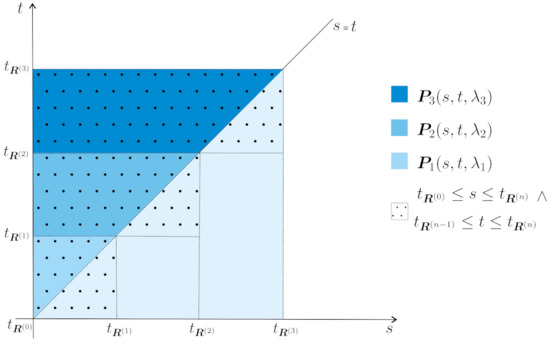
We observe that the definition in Formula (12) is coherent—see Figure 1—and then it is a simple verification with the definitions proposed. □

Figure 1. A representation of $\tilde{\mathit{P}}(s,t,\mathit{\lambda }\left(t\right))$ in Formula (12) for the first three initial times.

Remark 7

(An associated regime switching process). The function $\tilde{\mathit{P}}(s,t,\mathit{\lambda }\left(t\right))$ defined in Formula (12) was obtained by superimposing different transition probabilities for different Markov chains in continuous time. A natural question is to determine if there is—based on these different transitions probabilities—a regime switching Markov chain in continuous time that bears some connection with $\tilde{\mathit{P}}(s,t,\mathit{\lambda }\left(t\right))$. From a brief analysis of Figure 1 we can guess the natural definition of a regime switching Markov chain based on the probabilities ${\mathit{P}}_n(s,t,{\mathit{\lambda }}_{\mathit{n}})$. Let

$$\mathit{P}(s,t,\mathit{\lambda }\left(t\right)):={\mathit{P}}_n(s,t,{\mathit{\lambda }}_{\mathbf{n}}),t_{{\mathit{R}}^{(n-1)}}\le s\le t\le t_{{\mathit{R}}^{\left(n\right)}}.$$

(14)

Formula (14) has the following interpretation. For each $1\le n\le N$, consider continuous time Markov chain processes ${\left(X_t^n\right)}_{t\in [t_{{\mathit{R}}^{(n-1)}},t_{{\mathit{R}}^{\left(n\right)}}]}$ with transition probabilities ${\mathit{P}}_n(s,t,{\mathit{\lambda }}_{\mathbf{n}})$ defined in the domains ${\mathcal{R}}_n:=\{(s,t)\in {\mathbb{R}}^2:t_{{\mathit{R}}^{(n-1)}}\le s\le t\le t_{{\mathit{R}}^{\left(n\right)}}\}$ with the convention $t_{{\mathit{R}}^{\left(0\right)}}=0$. The regime switching process ${\left(Y_t\right)}_{t\in [0,t_{{\mathit{R}}^{\left(n\right)}}]}$ is such that (compare with Formula (2)):

$$Y_t=X_t^n,t\in [t_{{\mathit{R}}^{(n-1)}},t_{{\mathit{R}}^{\left(n\right)}}],$$

that is, the process ${\left(Y_t\right)}_{t\in [0,t_{{\mathit{R}}^{\left(n\right)}}]}$ is obtained by gluing together ${\left(X_t^n\right)}_{t\in [t_{{\mathit{R}}^{(n-1)}},t_{{\mathit{R}}^{\left(n\right)}}]}$, the paths of the processes which are bona fide continuous time Markov processes in each of their—non-random—time intervals $[t_{{\mathit{R}}^{(n-1)}},t_{{\mathit{R}}^{\left(n\right)}}]$. It is clear that $\mathit{P}(s,t,\mathit{\lambda }(t\left)\right)$ can be interpreted as a transition probability only when restricted to some domain ${\mathcal{R}}_n$ and that, in general, it will not be a transition probability in the whole interval $[0,t_{{\mathit{R}}^{\left(N\right)}}]$.

Remark 8.

The regime switching process defined in Remark 7 deserves further study. We may, nevertheless, define transition probabilities $\widehat{\mathit{P}}(s,t,\mathit{\lambda }\left(t\right))$ for $t_{{\mathit{R}}^{(k-1)}}\le s\le t_{{\mathit{R}}^{\left(k\right)}}\le t\le t_{{\mathit{R}}^{(k+1)}}$—with properties to be thoroughly investigated—by considering

$$\widehat{\mathit{P}}(s,t,\mathit{\lambda }\left(t\right)):={\mathit{P}}_k(s,t_{{\mathit{R}}^{\left(k\right)}},{\mathit{\lambda }}_{\mathbf{k}})·{\mathit{P}}_{k+1}(t_{{\mathit{R}}^{\left(k\right)}},t,{\mathit{\lambda }}_{\mathbf{k}+\mathbf{1}}).$$

3.3. Conclusions on the Relations between Embeddable Matrices, Calibration, and Open Markov Chain Models

From Theorems 1–3, the following conclusions can be drawn. Given a discrete time Markov transition matrix,

• if the matrix is embeddable—according to Definition 1 of Section 3.1—there is an unique in law homogeneous Markov chain in continuous time that solves the calibration problem optimally; the unicity is a consequence of Remark A2 that shows that the laws of the stopping times ${\left({\tau }_n\right)}_{n\ge 0}$ in the representation of Formula (A13) only depend on the intensities and these are uniquely determined whenever the discrete time Markov chain is embeddable.
• if the matrix is power-embeddable—that is, if all the matrices of a finite sequence with no gaps of powers of the matrix are embeddable—then there is an unique regime switching continuous time non-homogeneous Markov chain—in the sense of Remark 7—that solves the calibration problem optimally. In this case, the unicity has a justification similar to the previously referred case, that is, the laws of the stopping times only depends on the intensities and these are determined by the fact that the matrix is power-embeddable.

As a consequence, for our purposes, it appears of fundamental importance to determine if a discrete time Markov chain transition matrix is embeddable and to determine—if possible, explicitly—the embedding continuous time Markov chain. Regarding this problem the results in [43,55] deserve further consideration.

Remark 9

(Aplying Theorems 1–3). Suppose that discrete time Markov chain transition matrix, of a Markov chain process ${\left(Z_n\right)}_{n\ge 1}$ is embeddable in a continuous time Markov chain ${\left(X_t\right)}_{t\ge 0}$. We have, for this continuous time process and for a determined sequence of stopping times ${\left({\tau }_n\right)}_{n\ge 1}$, the representation given in Formula (A13) of Theorem A5, that is,

$$X_t=\sum _{n=0}^{+\infty }{X}_{{\tau }_n}1{\mathrm{I}}_{[{\tau }_n,{\tau }_{n+1}[}\left(t\right).$$

Now, as the Theorems referred to may consider that the process ${\left(Z_n\right)}_{n\ge 1}$ is suitably approximated by ${\left(X_t\right)}_{t\ge 0}$, we can also consider that the continuous time process defined by

$${\tilde{X}}_t:=\sum _{n=0}^{+\infty }{Z}_{{\tau }_n}1{\mathrm{I}}_{[{\tau }_n,{\tau }_{n+1}[}\left(t\right),$$

(15)

is an approximation of ${\left(Z_n\right)}_{n\ge 1}$ in continuous time. For processes with a structural representation similar to the one of the process ${\left({\tilde{X}}_t\right)}_{t\ge 0}$ we propose in Section 4.3 a method to extend from discrete to continuous time the open populations methodology.

4. More on Open Continuous Time Processes from Discrete Ones

In this section, we discuss an extension of the formalism of open Markov chains to the case of semi-Markov processes (sMp) and other continuous time processes, namely, the open Markov chain schemes introduced in [26]. For the reader’s convenience we present in Appendix B a short summary on sMp and in the next Section 4.1 a review of the main results on the open Markov chain formalism for discrete time. Finally, we propose the second main contribution of this work, that is, an extension of the open Markov chain formalism in discrete time to continuous time in the case of sMp. We also briefly refer the case of open Markov schemes that, in some particular instances, can be dealt as the sMp case.

4.1. Open Markov Chain Modeling in Discrete Time: A Short Review

We now detail and comment the results that will be used in this paper on discrete time open Markov chains. The study of open Markov chain models we will present next relies on results and notations that were introduced in [56], further developed in [22] and that we reproduce next, for the readers convenience. We will suppose that, in general, the transition matrix of the Markov chain model may be written in the following form:

$$\mathbf{P}=\left[\begin{array}{cc}\mathbf{K}\hfill & {\mathbf{U}}_1\hfill \\ \mathbf{0}\hfill & \mathbf{V}\hfill \end{array}\right]$$

(16)

where $\mathbf{K}$ is a $k\times k$ transition matrix between transient states, ${\mathbf{U}}_1$ a $k\times (r-k)$ matrix of transitions between the transient and the recurrent states, and $\mathbf{V}$ a $(r-k)\times (r-k)$ matrix of transitions between the recurrent states. A straightforward computation then shows that

$${\mathbf{P}}^{\left(n\right)}=\left[\begin{array}{cc}{\mathbf{K}}^{\left(n\right)}\hfill & {\mathbf{U}}_n\hfill \\ \mathbf{0}\hfill & {\mathbf{V}}^{\left(n\right)}\hfill \end{array}\right],n\in \mathbb{N}$$

with ${\mathbf{U}}_n={\mathbf{U}}_{n-1}\mathbf{V}+{\mathbf{K}}^{(n-1)}{\mathbf{U}}_1={\sum }_{i=0}^{n-1}{\mathbf{K}}^{\left(i\right)}{\mathbf{U}}_1{\mathbf{V}}^{(n-1-i)}$. We write the vector of the initial classification, for a time period i, as

$${\mathbf{c}}_i^{⊺}=\left[{\mathbf{t}}_i^{⊺}\left|{\mathbf{r}}_i^{⊺}\right],i\in \mathbb{N}\right.$$

(17)

with ${\mathbf{t}}_i$ the vector of the initial allocation probabilities for the transient states and ${\mathbf{r}}_i$ the vector of the initial allocation probabilities for the recurrent states. We suppose that at each epoch $i\ge 0$ there is an influx of new elements in the classes of the population—population that has its evolution governed by the Markov chain transition matrix—that is, a Poisson distributed with parameter ${\lambda }_i$. It is a consequence of the randomized sampling principle (see [57], pp. 216–217) that, if the incoming populations are distributed by the classes according with the multinomial distribution, then the sub-populations in the transient classes have independent Poisson distributions, with parameters given by the product of the Poisson parameter by the probability of the incoming new member being affected to the given class. With Formulas (16) and (17), we now notice that the vector of the Poisson parameters, for the population sizes in each state at an integer time N, may be written as

$${\mathit{\lambda }}_N^{++⊺}=\left[\sum _{i=1}^N{\lambda }_i{\mathbf{t}}_i^{⊺}{\mathbf{K}}^{(N-i)}\left|\sum _{i=1}^N{\lambda }_i\left({\mathbf{t}}_i^{⊺}{\mathbf{U}}_{N-i}+{\mathbf{r}}_i^{⊺}{\mathbf{V}}^{(N-i)}\right)\right]\right..$$

(18)

We observe that the first block corresponds to the transient states and the second block, the one in the right-hand side, corresponds to the recurrent states. From now on, as a first restricting hypothesis, we will also suppose that the transition matrix of the transient states, $\mathbf{K}$, is diagonalizable and so

$$\mathbf{K}=\sum _{j=1}^k{\eta }_j{\mathit{\alpha }}_j{\mathit{\beta }}_j^{⊺},$$

with ${\left({\eta }_j\right)}_{j\in \{1,\dots ,k\}}$ the eigenvalues, ${\left({\mathit{\alpha }}_j\right)}_{j\in \{1,\dots ,k\}}$ the left eigenvectors and ${\left({\mathit{\beta }}_j\right)}_{j\in \{1,\dots ,k\}}$ the right eigenvectors of matrix $\mathbf{K}$. We observe that $j\in \{1,\dots ,k\}$ corresponds to a transient state if and only if $\mid {\eta }_j\mid <1$. We may write the powers of $\mathbf{K}$ as

$${\mathbf{K}}^{\left(n\right)}=\sum _{j=1}^k{\eta }_j^n{\mathit{\alpha }}_j{\mathit{\beta }}_j^{⊺},$$

(19)

and so, as a consequence of (18), for the vector of the Poisson parameters corresponding only to the transient states, ${\mathit{\lambda }}_N^{+⊺}$, we have

$${\mathit{\lambda }}_N^{+⊺}=\sum _{i=1}^N{\lambda }_i{\mathbf{t}}_i^{⊺}{\mathbf{K}}^{(N-i)}=\sum _{j=1}^k\sum _{i=1}^N{\lambda }_i{\eta }_j^{N-i}{\mathbf{t}}_i^{⊺}{\mathit{\alpha }}_j{\mathit{\beta }}_j^{⊺}.$$

(20)

The main result describing the asymptotic behaviour, established in [22], is the following.

Theorem 4

(Asymptotic behavior of Poisson parameters of an open Markov chain with Poisson distributed influxes). Let a Markov chain driven system have a diagonalizable transition matrix between the transient states $\mathbf{K}={\sum }_{j=1}^k{\eta }_j{\mathit{\alpha }}_j{\mathit{\beta }}_j^{⊺}$, written in its spectral decomposition form. Suppose the system to be fed by Poisson inputs with intensities ${\left({\lambda }_i\right)}_{i\in \mathbb{N}}$ and such that the vector of initial classification of the inputs in the transient states converges to a fixed value, that is, ${\lim }_{i\to +\infty }{\mathbf{t}}_i^{⊺}={\mathbf{t}}_{\infty }^{⊺}\ne \mathbf{0}$. Then, with ${\mathit{\lambda }}_n^{+⊺}$ the vector of Poisson parameters of the transient sub-populations, at date $n\in \mathbb{N}$, we have the following:

1.

If ${\lim }_{n\to +\infty }{\lambda }_n=\lambda \in {\mathbb{R}}_{+}$, then

$${\mathit{\lambda }}_{\infty }^{+}=\underset{n\to +\infty }{\lim }{\mathit{\lambda }}_n^{+⊺}=\sum _{j=1}^k\frac{\mathit{\lambda }}{1-{\eta }_j}{\mathbf{t}}_{\infty }^{⊺}{\mathit{\alpha }}_j{\mathit{\beta }}_j^{⊺}.$$

(21)

2.

If ${\lim }_{n\to +\infty }{\lambda }_n=+\infty$ and there exists a constant $C>0$ such that

$$\underset{1\le i\le n}{\max }\left|\frac{{\lambda }_i-{\lambda }_{i+1}}{{\lambda }_n}\right|\le C$$

then

$$\underset{n\to +\infty }{\lim }\frac{{\mathit{\lambda }}_n^{+⊺}}{{\lambda }_n}=\sum _{j=1}^k\frac{1}{1-{\eta }_j}{\mathbf{t}}_{\infty }^{⊺}{\mathit{\alpha }}_j{\mathit{\beta }}_j^{⊺}.$$

(22)

Remark 10.

We observe that proportions in the Markov chain transient classes, on both statements of the Theorem 4, only depend on the eigenvalues ${\eta }_j,j=1,\dots ,k$. In fact, whenever using Formula (21) to compute proportions these proportions do not depend on the value of λ as we have that

$$\sum _{j=1}^k\frac{\lambda }{1-{\eta }_j}{\mathbf{t}}_{\infty }^{⊺}{\mathit{\alpha }}_j{\mathit{\beta }}_j^{⊺}=\lambda \left[{\mathbf{t}}_{\infty }^{⊺}·\left(\sum _{j=1}^k\frac{1}{1-{\eta }_j}{\mathit{\alpha }}_j{\mathit{\beta }}_j^{⊺}\right)\right],$$

and the term in the right-hand side multiplying λ is a vector with the dimension equal to the number of transient classes k, which is equal to the dimension of the square matrix $\mathbf{K}$. As so, when computing proportions, by normalizing this vector with the sum of its components, $\lambda \ne 0$ disappears.

4.2. Open sMP from Discrete time Open Markov Chains

Let us suppose that the successive Poisson distributions of the influx of new members in the population are independent of the random time at which the influx of new members in the population occurs. For the notations used, see Appendix B. Consider a sMp given by the representation in Formula (A17), that is,

$$Y_t=\sum _{n=0}^{+\infty }{Z}_{n}1{\mathrm{I}}_{[{\tau }_n,{\tau }_{n+1}[}\left(t\right),$$

in which ${\left(Z_n\right)}_{n\ge 0}$ is the embedded Markov chain and ${\left({\tau }_n\right)}_{n\ge 0}$ are the jump times of the process. We now propose a method to extend the known method to study open Markov chains in discrete time to sMps.

(1) 

In applications we usually consider that we have the influx of new members in the population being modeled by Poisson random variables that at each time t has a parameter $\lambda \left(t\right)$. Being so, Formula (20) may be rewritten as

$${\mathit{\lambda }}_N^{+⊺}=\sum _{i=1}^{i:t_i\le N}\lambda \left(t_i\right){\mathbf{t}}_i^{⊺}{\mathbf{K}}^{(N-i)}=\sum _{j=1}^k\sum _{i=1}^{i:t_i\le N}\lambda \left(t_i\right){\eta }_j^{N-i}{\mathbf{t}}_i^{⊺}{\mathit{\alpha }}_j{\mathit{\beta }}_j^{⊺},$$

(23)

where usually we can take $t_i=i$, as in a discrete time Markov chain, the actual time stamp is irrelevant as we only consider the sequence of epochs $i\ge 0$.

(2) 

In a sMp the only difference we have with respect to a discrete time Markov chain is that the dates ${\tau }_i$ corresponding to each epoch i are random; altogether, the structure of the changes in the sub-populations in the transient states is governed by the transition matrix of the Markov chain. In a sMp, the only possible observable changes are those that occur at the random times where it jumps; as so, we will suppose that the influxes of the new members of the population only occur at these random times. As a consequence, we should have that the vector parameter of the Poisson parameters, in the transient classes, is random since it depends on the random times in each we consider influxes and so, Formula (23) becomes

$${\mathit{\lambda }}_N^{+⊺}\left(\omega \right)=\sum _{i=1}^{i:{\tau }_i\left(\omega \right)\le N}\lambda \left({\tau }_i\left(\omega \right)\right){\mathbf{t}}_i^{⊺}{\mathbf{K}}^{(N-i)}=\sum _{j=1}^k\sum _{i=1}^{i:{\tau }_i\left(\omega \right)\le N}\lambda \left({\tau }_i\left(\omega \right)\right){\eta }_j^{N-i}{\mathbf{t}}_i^{⊺}{\mathit{\alpha }}_j{\mathit{\beta }}_j^{⊺}.$$

(24)

(3) 

The parameters of interest will be the expected values of the random variables ${\mathit{\lambda }}_N^{+⊺}\left(\omega \right)$—with the correspondent asymptotic behavior of these expected values when N grows indefinitely—and these expected values can be computed whenever the joint laws of $({\tau }_0,{\tau }_1,\dots ,{\tau }_i)$ are known, for $i\ge 0$. In fact, we observe that by Formula (24) we have

$$\begin{array}{cc}\hfill \mathbb{E}\left[{\mathit{\lambda }}_N^{+⊺}{\tau }_1,\dots {\tau }_i\dots \right]& =\mathbb{E}\left[\sum _{j=1}^k\sum _{i=1}^{i:{\tau }_i\le N}\lambda \left({\tau }_i\right){\eta }_j^{N-i}{\mathbf{t}}_i^{⊺}{\mathit{\alpha }}_j{\mathit{\beta }}_j^{⊺}{\tau }_1,\dots {\tau }_i\dots \right]=\hfill \\ \hfill & =\sum _{j=1}^k\sum _{i=1}^{i:{\tau }_i\le N}\lambda \left({\tau }_i\right){\eta }_j^{N-i}{\mathbf{t}}_i^{⊺}{\mathit{\alpha }}_j{\mathit{\beta }}_j^{⊺}.\hfill \end{array}$$

This formula has two consequences. The first one is that given an arbitrary strictly increasing sequence of dates $0=t_0<t_1<\dots <t_i<\dots$ we have

$$\mathbb{E}\left[{\mathit{\lambda }}_N^{+⊺}{\tau }_1=t_1,\dots {\tau }_i=t_i\dots \right]=\sum _{j=1}^k\sum _{i=1}^{i:t_i\le N}\lambda \left(t_i\right){\eta }_j^{N-i}{\mathbf{t}}_i^{⊺}{\mathit{\alpha }}_j{\mathit{\beta }}_j^{⊺},$$

thus justifying the assumption that given the strictly increasing of non accumulating stopping times dates $({\tau }_1=t_1,\dots {\tau }_i=t_i\dots )$ we can proceed as with the usual open Markov chain model in discrete time. The second consequence deserving mention is that in order to compute the expected value of the vector parameters of the transient classes sub-populations, while preserving the Poisson distribution of the influx new members, we compute

$$\mathbb{E}\left[{\mathit{\lambda }}_N^{+⊺}\right]=\mathbb{E}\left[\mathbb{E}\left[{\mathit{\lambda }}_N^{+⊺}{\tau }_1,\dots {\tau }_i\dots \right]\right]=\mathbb{E}\left[\sum _{j=1}^k\sum _{i=1}^{i:{\tau }_i\le N}\lambda \left({\tau }_i\right){\eta }_j^{N-i}{\mathbf{t}}_i^{⊺}{\mathit{\alpha }}_j{\mathit{\beta }}_j^{⊺}\right],$$

using the joint laws of $({\tau }_1,\dots ,{\tau }_i)$ for $i\ge 0$, laws we will suppose to be given.

Theorem 6, in the following, is one possible extension of the open Markov chain formalism to the sMp case taking as a starting point a discrete time Markov chain. To prove this result we will need Theorem 5—a generalization of Lebesgue dominated convergence theorem with varying measures—that we quote from Theorem 3.5 in [58] (p. 390).

Theorem 5

(Lebesgue dominated convergence theorem with varying measures). Consider $(\mathit{X},\mathcal{B}(\mathit{X}\left)\right)$ a locally compact, separable topological space endowed with its Borel σ-algebra. Suppose that the sequence of probability measures ${\left({\mu }_n\right)}_{n\ge 1}$—each one of them defined in $(\mathit{X},\mathcal{B}(\mathit{X}\left)\right)$—converges weakly to μ on $(\mathit{X},\mathcal{B}(\mathit{X}\left)\right)$ and that the sequence of measurable functions ${\left(f_n\right)}_{n\ge 1}$ converges continuously to f. Suppose additionally that, for some sequence of measurable functions ${\left(f_n\right)}_{n\ge 1}$ defined on $\mathit{X}$:

1.

For all $\mathbf{t}\in \mathit{X}$ and $n\ge 1$, we have that $\left|f_n\left(\mathbf{t}\right)\right|\le g_n\left(\mathbf{t}\right)$.

2.

With the function g defined on $\mathit{X}$ by

$$g\left(\mathit{t}\right):=\underset{{\left({\mathit{t}}_n\right)}_{n\ge 1},{\lim }_{n\to +\infty }{\mathit{t}}_n=\mathit{t}}{\inf }\left\{\underset{n\to +\infty }{\lim \inf }{g}_n\left({\mathit{t}}_n\right)\right\}$$

we have that

$$\underset{n\to +\infty }{\lim \sup }\int g_n\left(\mathit{t}\right)d{\mu }_n\left(\mathit{t}\right)\le \int g\left(\mathit{t}\right)d\mu \left(\mathit{t}\right)<+\infty .$$

Then, we have

$$\underset{n\to +\infty }{\lim }\int f_n\left(\mathit{t}\right)d{\mu }_n\left(\mathit{t}\right)=\int f\left(\mathit{t}\right)d\mu \left(\mathit{t}\right)<+\infty .$$

As said, we will suppose that we only observe the influx of the new members of the population into the sMp classes at the random times where it jumps—but, of course, accounting the state before the jump and the state after the jump—which is a hypothesis that makes sense under the perspective that we usually observe trajectories of the process. We then have the following extension of Theorem 4 to the case of sMp.

Theorem 6

(On the stability of open sMp transient states). Let a sMp given by the representation in Formula (A17), that is,

$$Y_t=\sum _{n=0}^{+\infty }{Z}_{n}1{\mathrm{I}}_{[{\tau }_n,{\tau }_{n+1}[}\left(t\right),$$

in which ${\left(Z_n\right)}_{n\ge 0}$ is the embedded Markov chain and ${\left({\tau }_i\right)}_{i\ge 0}$ are the jump times of the process. For the embedded Markov chain ${\left(Z_n\right)}_{n\ge 0}$, consider the notations of Section 4.2 and of Theorem 4 in this subsection. Suppose that the influx of new members in the population is modeled by Poisson random variables that at each time $t\in [0,+\infty [$ have a parameter $\mathit{\lambda }\left(t\right)$, with λ a continuousfunction. Suppose, furthermore, that the following hypothesis are verified.

1.

The stopping times ${\left({\tau }_i\right)}_{i\ge 0}$ are integrable, that is, $\mathbb{E}\left[{\tau }_i\right]<+\infty$ for all $i\ge 1$.

2.

There exists ${\lambda }_{\infty }>0$ such that, for every sequence of positive real numbers ${\left(t_i\right)}_{i\ge 1}$ such that ${\lim }_{i\to +\infty }{t}_i=+\infty$ we have

$$\underset{i\to +\infty }{\lim }\lambda \left(t_i\right)={\lambda }_{\infty }$$

(25)

Then, we have that the asymptotic behavior of the expected value vector of parameters of Poisson distributed sub-populations in the transient classes of an open sMp, submitted to a Poisson influx of new members at the jump times of the sMp, is given by

$$\underset{N\to +\infty }{\lim }\mathbb{E}\left[{\mathit{\lambda }}_N^{+⊺}\right]=\underset{N\to +\infty }{\lim }\mathbb{E}\left[\sum _{j=1}^k\sum _{i=1}^{i:{\tau }_i\le N}\lambda \left({\tau }_i\right){\eta }_j^{N-i}{\mathbf{t}}_i^{⊺}{\mathit{\alpha }}_j{\mathit{\beta }}_j^{⊺}\right]=\sum _{j=1}^k\frac{{\lambda }_{\infty }}{1-{\eta }_j}{\mathbf{t}}_{\infty }^{⊺}{\mathit{\alpha }}_j{\mathit{\beta }}_j^{⊺}.$$

(26)

Proof. 

For each $n\ge 1$, let $F_{({\tau }_1,\dots ,{\tau }_n)}$ be the joint distribution function of $({\tau }_1,\dots ,{\tau }_n)$. We want to compute the following limit of expectations:

$$\begin{array}{cc}\hfill \underset{N\to +\infty }{\lim }& \mathbb{E}\left[{\mathit{\lambda }}_N^{+⊺}\right]=\underset{N\to +\infty }{\lim }\mathbb{E}\left[{\lambda }_N^{+⊺},{\tau }_1<\dots <{\tau }_i\le N\right]=\hfill \\ \hfill & =\underset{N\to +\infty }{\lim }{\int }_{0<t_1<\dots <t_i\le N}{\mathit{\lambda }}_N^{+⊺}d{F}_{({\tau }_1,\dots ,{\tau }_n)}(t_1,\dots ,t_n)=\hfill \\ \hfill & =\underset{N\to +\infty }{\lim }{\int }_{0<t_1<\dots <t_i\le N}\left(\sum _{j=1}^k\sum _{i=1}^{i:t_i\le N}\lambda \left(t_i\right){\eta }_j^{N-i}{\mathbf{t}}_i^{⊺}{\mathit{\alpha }}_j{\mathit{\beta }}_j^{⊺}\right)d{F}_{({\tau }_1,\dots ,{\tau }_n)}(t_1,\dots ,t_n),\hfill \end{array}$$

(27)

and we observe that by Theorem 4 and by the first hypothesis, for every sequence of positive real numbers ${\left(t_i\right)}_{i\ge 1}$ such that ${\lim }_{i\to +\infty }{t}_i=+\infty$ and $t_1<t_2<\dots <t_i<\dots$, we have that

$$\underset{N\to +\infty }{\lim }\left(\sum _{j=1}^k\sum _{i=1}^{i:t_i\le N}\lambda \left(t_i\right){\eta }_j^{N-i}{\mathbf{t}}_i^{⊺}{\mathit{\alpha }}_j{\mathit{\beta }}_j^{⊺}\right)=\sum _{j=1}^k\frac{{\lambda }_{\infty }}{1-{\eta }_j}{\mathbf{t}}_{\infty }^{⊺}{\mathit{\alpha }}_j{\mathit{\beta }}_j^{⊺}.$$

(28)

The limit in the last term of Formula (27) requires a result of Lebesgue convergence theorem type but with varying measures. For the purpose of applying Theorem 5, we introduce the adequate context and notations and then we will apply the referred theorem. Consider the space $\mathit{X}={[0,+\infty [}^{{\aleph }_0}$ defined to be the space of infinite sequences of numbers in $[0,+\infty [$, that is,

$$\mathit{X}=\left\{\mathit{t}=(t_1,\dots ,t_i,\dots ):\forall i\ge 1,t_i\in [0,+\infty [\right\}.$$

Recall that with the metric d given by

$$\forall \mathit{t}=(t_1,\dots ,t_i,\dots ),{\mathit{t}}^{\prime }=(t_1^{\prime },\dots ,t_i^{\prime },\dots )\in \mathit{X},d(\mathit{t},{\mathit{t}}^{\prime }):=\sum _{i=1}^{+\infty }\frac{\min (1,\left|t_i-t_1^{\prime }\right|)}{2^i},$$

$\mathit{X}$ is a metric space, locally compact, separable and complete (see, for instance, in [59], pp. 9–10). We will consider $\mathit{X}={[0,+\infty [}^{{\aleph }_0}$ endowed with the Borel $\sigma$-algebra $\mathcal{B}\left(\mathit{X}\right)$ generated by the family ${\mathcal{P}}_f$ given by

$${\mathcal{P}}_f=\left\{A_{i_1}\times A_{i_2}\times \dots \times A_{i_p}:p\ge 1,A_{i_1}\in \mathcal{B}\left(\right[0,+\infty \left[\right)\right\},$$

with $\mathcal{B}\left(\right[0,+\infty \left[\right)$ the Borel $\sigma$-algebra of $[0,+\infty [$. We now take ${\left({\tau }_i\right)}_{i\ge 0}$ the sequence of the jump times of the process represented in Formula (A17). First, we define the sequence of measures ${\left({\mu }_n\right)}_{n\ge 1}$ where for each $n\ge 1$ we have that ${\mu }_n$ is defined on the measurable space ${\left(\right[0,+\infty [}^n,\mathcal{B}([0,+\infty {[}^n))$ by considering, for $A_1\times A_2\times \dots A_n$ with $A_i\in \mathcal{B}\left(\right[0,+\infty \left[\right)$, that

$${\mu }_n(A_1\times A_2\times \dots A_n)=\mathbb{P}\left[{\tau }_1\in A_1,\dots ,{\tau }_n\in A_n\right]={\int }_{t_1\in A_1,\dots ,t_n\in A_n}d{F}_{({\tau }_1,\dots ,{\tau }_n)}(t_1,\dots ,t_n).$$

(29)

Being so, ${\mu }_n$ is the probability joint law of $({\tau }_1,\dots ,{\tau }_n)$ and the last integral in the last term of Formula (27) is exactly an integration with respect to the measure ${\mu }_n$. As a consequence of Formula (29), the sequence ${\left({\mu }_n\right)}_{n\ge 1}$ verifies the compatibility conditions of Kolmogorov extension theorem (see [60], p. 46) and so there is a probability measure $\mathit{\mu }$, defined on $(\mathit{X},\mathcal{B}(\mathit{X}\left)\right)$, having as finite dimensional distributions the measures of the sequence ${\left({\mu }_n\right)}_{n\ge 1}$.

Now, for each $n\ge 1$, we can consider ${\tilde{\mu }}_n$ the extension of ${\mu }_n$ to the measurable space $(\mathit{X},\mathcal{B}(\mathit{X}\left)\right)$ in the following way:

$$\forall A\in \mathcal{B}\left(\mathit{X}\right){\tilde{\mu }}_n\left(A\right)={\int }_{\{\mathit{t}=(t_1,\dots ,t_i,\dots )\in A:t_1,\dots ,t_n\in [0,+\infty \left[\right\}}d{F}_{({\tau }_1,\dots ,{\tau }_n)}(t_1,\dots ,t_n).$$

(30)

In fact, with this definition the restriction of ${\tilde{\mu }}_n$ to $\mathcal{B}\left(\right[0,+\infty {[}^n)$ is exactly ${\mu }_n$. An important observation is the following. Consider $\mathbf{A}:=A_{i_1}\times A_{i_2}\times \dots \times A_{i_p}\in {\mathcal{P}}_f$. Then, for $m\ge i_p$ we have that

$$\begin{array}{cc}\hfill {\tilde{\mu }}_m\left(\mathit{A}\right)& ={\int }_{\{\mathit{t}=(t_1,\dots ,t_i,\dots )\in \mathit{A}:t_1,\dots ,t_m\in [0,+\infty \left[\right\}}d{F}_{({\tau }_1,\dots ,{\tau }_m)}(t_1,\dots ,t_m)=\hfill \\ \hfill & ={\int }_{\{\mathit{t}=(t_1,\dots ,t_i,\dots )\in \mathit{A}:t_1,\dots ,t_{i_p}\in [0,+\infty \left[\right\}}d{F}_{({\tau }_1,\dots ,{\tau }_{i_p})}(t_1,\dots ,t_{i_p})=\hfill \\ \hfill & ={\tilde{\mu }}_{i_p}\left(\mathit{A}\right)={\mu }_{i_p}\left(\mathit{A}\right)=\mu \left(\mathit{A}\right),\hfill \end{array}$$

(31)

thus showing that for every $\mathit{A}\in {\mathcal{P}}_f$ the sequence ${\left({\tilde{\mu }}_m\left(\mathit{A}\right)\right)}_{m\ge 1}$ converges to $\mathit{\mu }\left(\mathit{A}\right)$. Now, by Theorem 2.2 in [59] (p. 17), as ${\mathcal{P}}_f$ is a $\pi$-system and every open set in the metric space $(\mathit{X},d)$ is a countable union of elements of ${\mathcal{P}}_f$, we have that the sequence ${\left({\tilde{\mu }}_m\right)}_{m\ge 1}$ converges weakly to $\mu$. In order to apply Theorem 5 to compute the limit, we may consider two approaches to deal with the fact that ${\mathit{\lambda }}_N^{+⊺}$ is a vector of finite dimension k. Either we proceed component wise or we consider norms. Let us follow the second path. Define, for integer N, and some constant M,

$$f_N\left(\mathit{t}\right)=f_N(t_1,\dots ,t_i,\dots ):=\sum _{i=1}^{i:t_i\le N}\lambda \left(t_i\right){\eta }_j^{N-i}{\mathbf{t}}_i^{⊺}{\mathit{\alpha }}_j{\mathit{\beta }}_j^{⊺},$$

and also,

$$g_N\left(\mathit{t}\right)\equiv g:=∥\sum _{j=1}^k\frac{{\lambda }_{\infty }}{1-{\eta }_j}{\mathbf{t}}_{\infty }^{⊺}{\mathit{\alpha }}_j{\mathit{\beta }}_j^{⊺}∥+M,$$

in such a way that $∥f_N\left(\mathit{t}\right)∥\le g$; such choice of M is possible as a consequence of Formula (28). We can verify that the sequence ${\left(f_N\right)}_{N\ge 1}$ converges continuously to a function f by using Theorem 4.1.1 in [22] (p. 373). In fact, let us consider a sequence ${\left({\mathit{t}}_N\right)}_{n\ge 1}$ converging to some $({\mathit{t}}^{\infty }=(t_1^{\infty },\dots ,t_i^{\infty },\dots )$ in the metric space $(\mathit{X},d)$. With $({\mathit{t}}_N=(t_1^N,\dots ,t_i^N,\dots )$ we surely have that ${\lim }_{N\to +\infty }{t}_i^N=t_i^{\infty }$ for all $i\ge 1$. As a consequence of the continuity of $\mathit{\lambda }$ and of Theorem 4.1.1 in [22] (p. 373), we have that

$$\underset{N\to +\infty }{\lim }{f}_N\left({\mathit{t}}_N\right)=\underset{N\to +\infty }{\lim }\sum _{i=1}^{i:t_i^N\le N}\lambda \left(t_i^N\right){\eta }_j^{N-i}{\mathbf{t}}_i^{⊺}{\mathit{\alpha }}_j{\mathit{\beta }}_j^{⊺}=\sum _{j=1}^k\frac{\lambda \left({\lim }_{i\to +\infty }{t}_i^{\infty }\right)}{1-{\eta }_j}{\mathbf{t}}_{\infty }^{⊺}{\mathit{\alpha }}_j{\mathit{\beta }}_j^{⊺}=:f\left({\mathit{t}}^{\infty }\right).$$

It is clear now that the sequences ${\left(f_N\right)}_{N\ge 1}$, ${\left(g_N\right)}_{t\ge 1}$ and ${\left({\tilde{\mu }}_n\right)}_{n\ge 1}$ satisfy together with $\mathit{\mu }$ the hypothesis of Theorem 5 and so the announced result in Formula (25) follows. □

Remark 11

(Alternative proof for the weak convergence of the sequence ${\left({\tilde{\mu }}_n\right)}_{n\ge 1}$). There is another proof the weak convergence of the sequence ${\left({\tilde{\mu }}_m\right)}_{m\ge 1}$ to μ that we now present. We proceed by showing that the sequence ${\left({\tilde{\mu }}_n\right)}_{n\ge 1}$ is relatively compact—as a consequence of Prohorov theorem (see [59], pp. 59–63)—because, as we will show next, this sequence is tight. Let an arbitrary $0<ϵ<1$ be given and consider a sequence of positive numbers ${\left({\xi }_i\right)}_{i\ge 1}$ such that, by Tchebychev inequality and using the fact that the stopping times ${\tau }_i$ have finite integrals,

$$\mathbb{P}\left[{\tau }_i>{\xi }_i\right]\le \frac{\mathbb{E}\left[{\tau }_i\right]}{{\xi }_i},$$

in such a way that

$$\sum _{i=1}^{+\infty }\frac{\mathbb{E}\left[{\tau }_i\right]}{{\xi }_i}<ϵ.$$

Now consider the Borel set $K_{ϵ}={\prod }_{i=1}^{+\infty }[0,{\xi }_i]\subset \mathit{X}$ which is compact by Tychonov theorem. We now have that

$$\begin{array}{cc}\hfill {\tilde{\mu }}_n\left(K_{ϵ}\right)& ={\int }_{\{\mathit{t}=(t_1,\dots ,t_i,\dots )\in K_{ϵ}:t_1,\dots ,t_n\in [0,+\infty \left[\right\}}d{F}_{({\tau }_1,\dots ,{\tau }_n)}(t_1,\dots ,t_n)=\hfill \\ \hfill & ={\int }_{{\prod }_{i=1}^n[0,{\xi }_i]}d{F}_{({\tau }_1,\dots ,{\tau }_n)}(t_1,\dots ,t_n)=\hfill \\ \hfill & =\mathbb{P}\left[({\tau }_1,\dots ,{\tau }_n)\in \prod _{i=1}^n[0,{\xi }_i]\right]=\mathbb{P}\left[\bigcap _{i=1}^n\{{\tau }_i\le {\xi }_i\}\right]=1-\mathbb{P}\left[\bigcup _{i=1}^n\{{\tau }_i>{\xi }_i\}\right]\ge \hfill \\ \hfill & \ge 1-\sum _{i=1}^n\frac{\mathbb{E}\left[{\tau }_i\right]}{{\xi }_i}\ge 1-\sum _{i=1}^{+\infty }\frac{\mathbb{E}\left[{\tau }_i\right]}{{\xi }_i}\ge 1-ϵ,\hfill \end{array}$$

thus showing that the sequence of probability measures ${\left({\tilde{\mu }}_n\right)}_{n\ge 1}$ is tight in the measurable space $(\mathit{X},\mathcal{B}(\mathit{X}\left)\right)$. As said, by Prokhorov’s theorem, this implies that the sequence ${\left({\tilde{\mu }}_n\right)}_{n\ge 1}$ is relatively compact, that is, for every subsequence of ${\left({\tilde{\mu }}_n\right)}_{n\ge 1}$, there exists a further subsequence and a probability measure such that this subsequence converges weakly to the said probability measure. Now, as, by construction, the probability measure μ has, as finite dimensional distributions the probability measures ${\left({\tilde{\mu }}_n\right)}_{n\ge 1}$ we can say that for $n\ge 1$, the finite dimensional distributions of ${\tilde{\mu }}_n$ converge weakly to the finite dimensional distributions of μ. As a consequence, following the observation in [59] (p. 58), the sequence ${\left({\tilde{\mu }}_n\right)}_{n\ge 1}$ converges weakly to μ.

Remark 12

(Applying Theorem 6). If we manage to estimate a discrete time Markov chain transition matrix and if we manage to fit some function f—such that ${\lim }_{t\to +\infty }f\left(t\right)={\lambda }_{\infty }$—to the number of new incoming members in the population at a set of non accumulating non-evenly spaced dates (as done with a statistical procedure in [22] or, with a simple fitting in [25]) then, Theorem 6 allows us to get the asymptotic expected number of elements in the transient classes of a sMp having as embedded Markov chain the estimated one.

4.3. Open Continuous Time Processes from Open Markov Schemes

We may follow the approach of open Markov schemes in [26] and define a process in continuous time after getting a process in random discrete times describing, at least on average, the evolution of the elements in each transient class. Let us briefly recall the main idea. A population model is driven by a Markov chain defined by a sequence of initial distributions given, for $n\ge 1$, by ${\left({\mathbf{q}}^n\right)}^{⊺}=(q_1^n,q_2^n,\dots ,q_{r_{☆}}^n)$ and a transition matrix $\mathbf{P}=\left[p_{ij}\right],1\le i,j\le r$. After the first transition, the new values of the proportions in all states, after one transition, can be recovered from ${\mathbf{P}}^{⊺}\mathbf{q}={\left({\mathbf{q}}^{⊺}\mathbf{P}\right)}^{⊺}$ and, after n transitions, by ${\left({\mathbf{P}}^{\left(n\right)}\right)}^{⊺}\mathbf{q}={\left({\mathbf{q}}^{⊺}{\mathbf{P}}^{\left(n\right)}\right)}^{⊺}$. We want to account for the evolution of the expected number of elements in each class supposing that, at each random date ${\tau }_k$, a random number $X_{{\tau }_k}$ of new elements enters the population. Just after the second cohort enters the population, a first transition occurs in the first cohort driven by the Markov chain law and so on and so forth. Table 1 summarizes this accounting process in which, at each step k, we distribute multinomially the new random arrivals $X_{{\tau }_k}$ according to the probability vector ${\mathbf{q}}^k$ and the elements in each class are redistributed according to the Markov chain transition matrix $\mathbf{P}$.

Table 1. Accounting of n Markov cohorts each with an initial distribution.

Date	${\mathit{\tau }}_1$	${\mathit{\tau }}_2$	⋯	${\mathit{\tau }}_{\mathit{n}-1}$	${\mathit{\tau }}_{\mathit{n}}$
${\tau }_1$	$\mathbb{E}\left[X_{{\tau }_1}\right]{\left({\mathbf{q}}^1\right)}^{⊺}$	$\mathbb{E}\left[X_{{\tau }_1}\right]{\left({\mathbf{q}}^1\right)}^{⊺}\mathbf{P}$	⋯	$\mathbb{E}\left[X_{{\tau }_1}\right]{\left({\mathbf{q}}^1\right)}^{⊺}{\mathbf{P}}^{(n-2)}$	$\mathbb{E}\left[X_{{\tau }_1}\right]{\left({\mathbf{q}}^1\right)}^{⊺}{\mathbf{P}}^{(n-1)}$
${\tau }_2$	–	$\mathbb{E}\left[X_{{\tau }_2}\right]{\left({\mathbf{q}}^2\right)}^{⊺}$	⋯	$\mathbb{E}\left[X_{{\tau }_2}\right]{\left({\mathbf{q}}^2\right)}^{⊺}{\mathbf{P}}^{(n-3)}$	$\mathbb{E}\left[X_{{\tau }_2}\right]{\left({\mathbf{q}}^2\right)}^{⊺}{\mathbf{P}}^{(n-2)}$
⋯	⋯	⋯	⋯	⋯	⋯
${\tau }_n$	–	–	–	–	$\mathbb{E}\left[X_{{\tau }_n}\right]{\left({\mathbf{q}}^n\right)}^{⊺}$

At date ${\tau }_k$, if we suppose that each new set of individuals in the population, a cohort, evolves independently from any one of the already existing sets of individuals but, accordingly, to the same Markov chain model, we may recover the total expected number of elements in each class at date ${\tau }_k$ by computing the sum:

$$\begin{array}{c}\hfill {\overline{\mathbf{K}}}_n=\sum _{k=1}^n\mathbb{E}\left[X_{{\tau }_k}\right]{\left({\mathbf{q}}^k\right)}^{⊺}{\mathbf{P}}^{(n-k)}.\end{array}$$

(32)

Each vector component corresponds precisely to the expected number of elements in each class. In order to further study the properties of ${\left({\overline{\mathbf{K}}}_n\right)}_{n\ge 1}$, given the properties of a stochastic process $\mathbb{X}={\left(X_{{\tau }_k}\right)}_{k\ge 1}$, we will randomize formula (32) by considering, instead, for $n\ge 1$:

$${\mathbf{K}}_n=\sum _{k=1}^n{X}_{{\tau }_k}{\left({\mathbf{q}}^k\right)}^{⊺}{\mathbf{P}}^{(n-k)},$$

(33)

and we observe that in any case $\mathbb{E}\left[\mathbf{K}\right]={\overline{\mathbf{K}}}_n$. It is known that if the vector of classification probabilities is constant ${\mathbf{c}}^k=\mathbf{c}$ and if the $\mathbb{X}$ is an ARMA, ARIMA, or SARIMA process, then the populations in each of the transient classes can be described by a sum of a deterministic trend, plus an ARMA process plus an evanescent process, that is a centered process ${\left(Y_k\right)}_{k\ge 1}$ such that ${\lim }_{k\to +\infty }\mathbb{E}\left[{\left|Y_k\right|}^2\right]=0$ (see Theorems 3.1 and 3.2 in [26]).

The step process in continuous time naturally associated with the discrete time one would be then defined by for $t\ge 0$ by

$${\mathbf{K}}_t:=\sum _{n=0}^{+\infty }{\mathbf{K}}_{n}1{\mathrm{I}}_{[{\tau }_n,{\tau }_{n+1}[}\left(t\right)=\sum _{n=0}^{+\infty }\left(\sum _{k=1}^n{X}_{{\tau }_k}{\left({\mathbf{q}}^k\right)}^{⊺}{\mathbf{P}}^{(n-k)}\right)1{\mathrm{I}}_{[{\tau }_n,{\tau }_{n+1}[}\left(t\right).$$

In order to study this process we will have to take advantage of the properties of $\mathbb{X}$ and of the family of stopping times ${\left({\tau }_k\right)}_{k\ge 0}$. It should be noticed that if the process $\mathbb{X}={\left(X_t\right)}_{t\ge 0}$ is Poisson distributed and the laws of the sequence ${\left({\tau }_k\right)}_{k\ge 0}$ are known and it possible to determine the expected value of ${\mathbf{K}}_t$ for $t\ge 0$ with a result similar to Theorem 6.

5. Conclusions

In this work, we studied several ways to associate, to an open Markov chain process in discrete time—which is often the sole accessible fruit of observation—a continuous time Markov or semi-Markov process that bears some natural relation with the discrete time process. Furthermore, we expect that association to allow the extension of the study of open populations from the discrete to the continuous time model. For that purpose, we consider three approaches: the first, for the continuous time Markov chains; the second, for the semi Markov case; and the third, for the open Markov schemes (see in [26]). For the semi-Markov case, under the hypothesis that we only observe the influx of new individuals in the population at the times of the random jumps, in the main result we determine the expected value of the vector of parameters of the conditional Poisson distributions in the transient classes when the influx of new members is Poisson distributed. The third approach, dealing with open Markov schemes is similar to the second one whenever we consider a similar context hypothesis, that is, distributed incoming new members of the population with known distributions and observation of this influx of new individuals at the times of the random jumps. In the case of the first approach, that is, for the case of Markov chain in continuous time, we propose a calibration procedure for which the embeddable Markov chains provide optimal solutions. In this case also, the study of open populations models relies on the main result proved for the semi-Markov case approach. Future work encompasses applications to real data and the determination of criteria to assess the quality of the association of the continuous model to the observed discrete time model.

References

- Vajda, S. The stratified semi-stationary population. Biometrika 1947, 34, 243–254. [Google Scholar] [CrossRef] [PubMed]
- Young, A.; Almond, G. Predicting Distributions of Staff. Comput. J. 1961, 3, 246–250. [Google Scholar] [CrossRef][Green Version]
- Bartholomew, D.J. A multi-stage renewal process. J. R. Statist. Soc. Ser. B 1963, 25, 150–168. [Google Scholar] [CrossRef]
- Bartholomew, D.J. Stochastic Models for Social Processes, 2nd ed.; Wiley Series in Probability and Mathematical Statistics; John Wiley & Sons: London, UK; New York, NY, USA; Sydney, Australia, 1973. [Google Scholar]
- Bartholomew, D.J. Stochastic Models for Social Processes, 3rd ed.; Wiley Series in Probability and Mathematical Statistics; John Wiley & Sons, Ltd.: Chichester, UK, 1982. [Google Scholar]
- Gani, J. Formulae for Projecting Enrolments and Degrees Awarded in Universities. J. R. Stat. Soc. Ser. A 1963, 126, 400–409. [Google Scholar] [CrossRef]
- Bowerman, B.; David, H.T.; Isaacson, D. The convergence of Cesaro averages for certain nonstationary Markov chains. Stoch. Process. Appl. 1977, 5, 221–230. [Google Scholar] [CrossRef][Green Version]
- Vassiliou, P.C.G. Cyclic behaviour and asymptotic stability of nonhomogeneous Markov systems. J. Appl. Probab. 1984, 21, 315–325. [Google Scholar] [CrossRef]
- Vassiliou, P.C.G. Asymptotic variability of nonhomogeneous Markov systems under cyclic behaviour. Eur. J. Oper. Res. 1986, 27, 215–228. [Google Scholar] [CrossRef]
- Dimitriou, V.A.; Georgiou, A.C. Introduction, analysis and asymptotic behavior of a multi-level manpower planning model in a continuous time setting under potential department contraction. Commun. Statist. Theory Methods 2021, 50, 1173–1199. [Google Scholar] [CrossRef]
- Salgado-García, R. Open Markov Chains: Cumulant Dynamics, Fluctuations and Correlations. Entropy 2021, 23, 256. [Google Scholar] [CrossRef]
- Vassiliou, P.C.G.; Papadopoulou, A.A. Nonhomogeneous semi-Markov systems and maintainability of the state sizes. J. Appl. Probab. 1992, 29, 519–534. [Google Scholar] [CrossRef]
- Papadopoulou, A.A.; Vassiliou, P.C.G. Asymptotic behavior of nonhomogeneous semi-Markov systems. Linear Algebra Appl. 1994, 210, 153–198. [Google Scholar] [CrossRef]
- Vassiliou, P.C.G. Asymptotic Behavior of Markov Systems. J. Appl. Probab. 1982, 19, 851–857. [Google Scholar] [CrossRef]
- Vassiliou, P.C.G. Markov Systems in a General State Space. Commun. Stat. Theory Methods 2014, 43, 1322–1339. [Google Scholar] [CrossRef]
- Vassiliou, P.-C.G. Rate of Convergence and Periodicity of the Expected Population Structure of Markov Systems that Live in a General State Space. Mathematics 2020, 8, 1021. [Google Scholar] [CrossRef]
- Vassiliou, P.-C.G. Non-Homogeneous Markov Set Systems. Mathematics 2021, 9, 471. [Google Scholar] [CrossRef]
- McClean, S.I. A continuous-time population model with Poisson recruitment. J. Appl. Probab. 1976, 13, 348–354. [Google Scholar] [CrossRef]
- McClean, S.I. Continuous-time stochastic models of a multigrade population. J. Appl. Probab. 1978, 15, 26–37. [Google Scholar] [CrossRef]
- McClean, S.I. A Semi-Markov Model for a Multigrade Population with Poisson Recruitment. J. Appl. Probab. 1980, 17, 846–852. [Google Scholar] [CrossRef]
- Papadopoulou, A.A.; Vassiliou, P.C.G. Continuous time nonhomogeneous semi-Markov systems. In Semi-Markov Models and Applications (Compiègne, 1998); Kluwer Academic Publishers: Dordrecht, The Netherlands, 1999; pp. 241–251. [Google Scholar]
- Esquível, M.L.; Fernandes, J.M.; Guerreiro, G.R. On the evolution and asymptotic analysis of open Markov populations: Application to consumption credit. Stoch. Models 2014, 30, 365–389. [Google Scholar] [CrossRef]
- Guerreiro, G.R.; Mexia, J.A.T.; de Fátima Miguens, M. Statistical approach for open bonus malus. Astin Bull. 2014, 44, 63–83. [Google Scholar] [CrossRef]
- Afonso, L.B.; Cardoso, R.M.R.; Egídio dos Reis, A.D.; Guerreiro, G.R. Ruin Probabilities And Capital Requirement for Open Automobile Portfolios With a Bonus-Malus System Based on Claim Counts. J. Risk Insur. 2020, 87, 501–522. [Google Scholar] [CrossRef]
- Esquível, M.L.; Patrício, P.; Guerreiro, G.R. From ODE to Open Markov Chains, via SDE: An application to models for infections in individuals and populations. Comput. Math. Biophys. 2020, 8, 180–197. [Google Scholar] [CrossRef]
- Esquível, M.; Guerreiro, G.; Fernandes, J. Open Markov chain scheme models. REVSTAT 2017, 15, 277–297. [Google Scholar]
- Esquível, M.L.; Guerreiro, G.R.; Oliveira, M.C.; Corte Real, P. Calibration of Transition Intensities for a Multistate Model: Application to Long-Term Care. Risks 2021, 9, 37. [Google Scholar] [CrossRef]
- Resnick, S.I. Adventures in Stochastic Processes; Birkhäuser: Boston, MA, USA, 1992. [Google Scholar]
- Rolski, T.; Schmidli, H.; Schmidt, V.; Teugels, J. Stochastic Processes for Insurance and Finance; Wiley Series in Probability and Statistics; John Wiley & Sons Ltd.: Chichester, UK, 1999. [Google Scholar] [CrossRef]
- Iosifescu, M. Finite Markov Processes and Their Applications; Wiley Series in Probability and Mathematical Statistics; JohnWiley & Sons, Ltd.: Chichester, UK; Editura Tehnică: Bucharest, Romania, 1980; p. 295. [Google Scholar]
- Iosifescu, M.; Tăutu, P. Stochastic Processes and Applications in Biology and Medicine. I: Theory; Biomathematics; Editura Academiei RSR: Bucharest, Romania; Springer: Berlin, Germany; New York, NY, USA, 1973; Volume 3, p. 331. [Google Scholar]
- Pyke, R. Markov renewal processes: Definitions and preliminary properties. Ann. Math. Statist. 1961, 32, 1231–1242. [Google Scholar] [CrossRef]
- Korolyuk, V.S.; Korolyuk, V.V. Stochastic Models of Systems. In Mathematics and its Applications; Kluwer Academic Publishers: Dordrecht, The Netherlands, 1999; Volume 469. [Google Scholar] [CrossRef]
- Kingman, J.F.C. The imbedding problem for finite Markov chains. Probab. Theory Relat. Fields 1962, 1, 14–24. [Google Scholar] [CrossRef]
- Johansen, S. The Imbedding Problem for Finite Markov Chains. In Geometric Methods in System Theory, 1st ed.; Mayne, D.Q.B.R.W., Ed.; D. Reidel Publishing Company: Dordrecht, The Netherlands; Boston, MA, USA, 1973; Volume 1, Chapter 13; pp. 227–237. [Google Scholar]
- Johansen, S. A central limit theorem for finite semigroups and its application to the imbedding problem for finite state Markov chains. Z. Wahrscheinlichkeitstheorie Verw. Gebiete 1973, 26, 171–190. [Google Scholar] [CrossRef]
- Johansen, S. Some Results on the Imbedding Problem for Finite Markov Chains. J. Lond. Math. Soc. 1974, 2, 345–351. [Google Scholar] [CrossRef]
- Fuglede, B. On the imbedding problem for stochastic and doubly stochastic matrices. Probab. Theory Relat. Fields 1988, 80, 241–260. [Google Scholar] [CrossRef]
- Guerry, M.A. On the Embedding Problem for Discrete-Time Markov Chains. J. Appl. Probab. 2013, 50, 918–930. [Google Scholar] [CrossRef]
- Jia, C. A solution to the reversible embedding problem for finite Markov chains. Stat. Probab. Lett. 2016, 116, 122–130. [Google Scholar] [CrossRef]
- Goodman, G.S. An intrinsic time for non-stationary finite Markov chains. Probab. Theory Relat. Fields 1970, 16, 165–180. [Google Scholar] [CrossRef]
- Singer, B. Estimation of Nonstationary Markov Chains from Panel Data. Sociol. Methodol. 1981, 12, 319–337. [Google Scholar] [CrossRef]
- Lencastre, P.; Raischel, F.; Rogers, T.; Lind, P.G. From empirical data to time-inhomogeneous continuous Markov processes. Phys. Rev. E 2016, 93, 032135. [Google Scholar] [CrossRef]
- Ekhosuehi, V.U. On the use of Cauchy integral formula for the embedding problem of discrete-time Markov chains. Commun. Stat. Theory Methods 2021, 1–15. [Google Scholar] [CrossRef]
- Coddington, E.A.; Levinson, N. Theory of Ordinary Differential Equations; McGraw-Hill Book Company, Inc.: New York, NY, USA; Toronto, ON, Canada; London, UK, 1955. [Google Scholar]
- Rudin, W. Real and Complex Analysis, 3rd ed.; McGraw-Hill Book Co.: New York, NY, USA, 1987. [Google Scholar]
- Kurzweil, J. Ordinary differential equations. In Studies in Applied Mechanics; Introduction to the theory of ordinary differential equations in the real domain, Translated from the Czech by Michal Basch; Elsevier Scientific Publishing Co.: Amsterdam, The Netherlands, 1986; Volume 13, p. 440. [Google Scholar]
- Teschl, G. Ordinary differential equations and dynamical systems. In Graduate Studies in Mathematics; American Mathematical Society: Providence, RI, USA, 2012; Volume 140. [Google Scholar] [CrossRef]
- Nevanlinna, F.; Nevanlinna, R. Absolute Analysis; Translated from the German by Phillip Emig, Die Grundlehren der mathematischen Wissenschaften, Band 102; Springer: New York, NY, USA; Heidelberg, Germany, 1973. [Google Scholar]
- Severi, F.; Scorza Dragoni, G. Lezioni di analisi. Vol. 3. Equazioni Differenziali Ordinarie e Loro Sistemi, Problemi al Contorno Relativi, Serie Trigonometriche, Applicazioni Geometriche; Cesare Zuffi: Bologna, Italy, 1951. [Google Scholar]
- Dobrušin, R.L. Generalization of Kolmogorov’s equations for Markov processes with a finite number of possible states. Matematicheskii Sbornik 1953, 33, 567–596. [Google Scholar]
- Pritchard, D.J. Modeling Disability in Long-Term Care Insurance. N. Am. Actuar. J. 2006, 10, 48–75. [Google Scholar] [CrossRef]
- Kingman, J.F.C. Ergodic properties of continuous-time Markov processes and their discrete skeletons. Proc. Lond. Math. Soc. 1963, 13, 593–604. [Google Scholar] [CrossRef]
- Conner, H. A note on limit theorems for Markov branching processes. Proc. Am. Math. Soc. 1967, 18, 76–86. [Google Scholar] [CrossRef]
- Israel, R.B.; Rosenthal, J.S.; Wei, J.Z. Finding generators for Markov chains via empirical transition matrices, with applications to credit ratings. Math. Financ. 2001, 11, 245–265. [Google Scholar] [CrossRef]
- Guerreiro, G.R.; Mexia, J.A.T. Stochastic vortices in periodically reclassified populations. Discuss. Math. Probab. Stat. 2008, 28, 209–227. [Google Scholar] [CrossRef][Green Version]
- Feller, W. An Introduction to Probability Theory and Its Applications. Vol. I, 3rd ed.; John Wiley & Sons, Inc.: New York, NY, USA; London, UK; Sydney, Australia, 1968. [Google Scholar]
- Serfozo, R. Convergence of Lebesgue integrals with varying measures. Sankhyā Ser. A 1982, 44, 380–402. [Google Scholar]
- Billingsley, P. Convergence of Probability Measures, 2nd ed.; Wiley Series in Probability and Statistics: Probability and Statistics; John Wiley & Sons, Inc.: New York, NY, USA, 1999. [Google Scholar] [CrossRef]
- Durrett, R. Probability—Theory and Examples. In Cambridge Series in Statistical and Probabilistic Mathematics; Cambridge University Press: Cambridge, UK, 2019; Volume 49. [Google Scholar] [CrossRef]
- Skorokhod, A.V. Lectures on the Theory of Stochastic Processes; VSP: Utrecht, The Netherlands; TBiMC Scientific Publishers: Kiev, Ukraine, 1996. [Google Scholar]
- Dynkin, E.B. Theory of Markov Processes; Translated from the Russian by D. E. Brown and edited by T. Köváry, Reprint of the 1961 English translation; Dover Publications, Inc.: Mineola, NY, USA, 2006. [Google Scholar]
- Iosifescu, M.; Limnios, N.; Oprişan, G. Introduction to Stochastic Models; Applied Stochastic Methods Series; Translated from the 2007 French original by Vlad Barbu; ISTE: London, UK; John Wiley & Sons, Inc.: Hoboken, NJ, USA, 2010. [Google Scholar] [CrossRef]
- Pyke, R. Markov renewal processes with finitely many states. Ann. Math. Statist. 1961, 32, 1243–1259. [Google Scholar] [CrossRef]
- Feller, W. On semi-Markov processes. Proc. Nat. Acad. Sci. USA 1964, 51, 653–659. [Google Scholar] [CrossRef]
- Kurtz, T.G. Comparison of semi-Markov and Markov processes. Ann. Math. Statist. 1971, 42, 991–1002. [Google Scholar] [CrossRef]
- Korolyuk, V.; Swishchuk, A. Semi-Markov random evolutions. In Mathematics and its Applications; Translated from the 1992 Russian original by V. Zayats and revised by the authors; Kluwer Academic Publishers: Dordrecht, The Netherlands, 1995; Volume 308. [Google Scholar] [CrossRef]
- Janssen, J.; de Dominicis, R. Finite non-homogeneous semi-Markov processes: Theoretical and computational aspects. Insur. Math. Econ. 1984, 3, 157–165. [Google Scholar] [CrossRef]
- Janssen, J.; Limnios, N. (Eds.) Semi-Markov Models and Applications; Selected papers from the 2nd International Symposium on Semi-Markov Models: Theory and Applications held in Compiègne, December 1998; Kluwer Academic Publishers: Dordrecht, The Netherlands, 1999. [Google Scholar] [CrossRef]
- Janssen, J.; Manca, R. Applied Semi-Markov Processes; Springer: New York, NY, USA, 2006. [Google Scholar]
- Janssen, J.; Manca, R. Semi-Markov Risk Models for Finance, Insurance and Reliability; Springer: New York, NY, USA, 2007. [Google Scholar]
- Barbu, V.S.; Limnios, N. Semi-Markov chains and hidden semi-Markov models toward applications. In Lecture Notes in Statistics; Springer: New York, NY, USA, 2008; Volume 191. [Google Scholar]
- Grabski, F. Semi-Markov Processes: Applications in System Reliability and Maintenance; Elsevier: Amsterdam, The Netherlands, 2015. [Google Scholar]
- Ross, S.M. Applied Probability Models with Optimization Applications; Reprint of the 1970 original; Dover Publications, Inc.: New York, NY, USA, 1992. [Google Scholar]
- Moore, E.H.; Pyke, R. Estimation of the transition distributions of a Markov renewal process. Ann. Inst. Stat. Math. 1968, 20, 411. [Google Scholar] [CrossRef]
- Ouhbi, B.; Limnios, N. Nonparametric Estimation for Semi-Markov Processes Based on its Hazard Rate Functions. Stat. Inference Stoch. Process. 1999, 2, 151–173. [Google Scholar] [CrossRef]
Publisher’s Note: MDPI stays neutral with regard to jurisdictional claims in published maps and institutional affiliations. |
© 2021 by the authors. Licensee MDPI, Basel, Switzerland. This article is an open access article distributed under the terms and conditions of the Creative Commons Attribution (CC BY) license (https://creativecommons.org/licenses/by/4.0/).