Co-Movements between Eu Ets and the Energy Markets: A Var-Dcc-Garch Approach

Abstract

This paper analyzes the co-movements of prices of fossil fuels, energy stock markets and EU allowances. This analysis is conducted in order to identify the spillover effect of volatility and correlation among these financial markets, and to provide a scientific basis that shows the interest of incorporating sustainable assets in the design of minimum risk strategies of investment. To achieve this goal, we have used a Vector Autoregressive-Dynamic Conditional Correlation-Generalized Autoregressive Conditional Heteroscedasticity (VAR-DCC-GARCH) model that also incorporates a stock index of industrial companies as a leading indicator of the level of economic activity. In addition, the paper conducts an impulse response analysis to determine how unexpected shocks to prices are propagated along time, and, in particular, how they affect prices of the others, both in mean, variance and correlation. Therefore, the results of this one- and two-dimensional analysis allow for the study of short and long run dynamics of the relationship among those prices, thus, providing greater meaning and information for investors, which has implications for building their portfolios. The analyzed period was from January 2010 to February 2021, so that the data include half of phase II, full phase III and the onset of phase IV of the EU ETS, as well as the COVID-19 outbreak in the European context. We also analyzed whether the EUA price impulses the demand of clean energy stocks, which has important implications for the objective of triggering the investment in clean energy. Our results show the transmission mechanism of all of those prices, which are relevant not only for investors but also for policymakers to construct an early-warning system, revealing the most important transmission channels. Moreover, from an investment viewpoint, we observe a decline in dirty energies and a rise in the clean energy market, which might be an indication of the progress towards the energy transition to renewables sources within a circular economy perspective. Therefore, this shows that the EU ETS is achieving its goals, and that clean energy companies, aligned with their role towards socially responsible initiatives, are also gaining acceptance in terms of investments, which would be beneficial for the environment.

1. Introduction

Climate change has deeply influenced environmental issues, the economy and human health in the world. Greenhouse gas (GHG) emissions are the main source of climate change and global warming. Confronted with this situation, many countries and regions implemented the emission trading scheme, to achieve emission mitigation goals set by the Kyoto Protocol, Copenhagen Accord and Paris agreement.

The EU emissions trading system (EU ETS) is the cornerstone of the EU’s policy to combat climate change, and its key tool for reducing GHG emissions cost-effectively. The EU ETS works on the ‘cap and trade’ principle. Within the cap (set as the total amount of gases that can be emitted by installations covered by the system), companies receive or buy emission allowances, which they can trade with one another as needed. The EU ETS operates by setting a cap on CO₂ emissions, which generates a price that reflects the scarcity in the market.

The EU ETS was divided into four phases (phase I: 2005–2007, phase II: 2008–2012, phase III: 2013–2020), and the fourth phase (2021–2030), has just begun. In phase I and phase II, the cap was established bottom-up, based on the aggregation of the national allocation plans of each member state. Phase III started with a single EU-wide cap for stationary sources, which was annually reduced by a linear factor of 1.74%. As a result, in 2014, the commitment to reduce CO₂ emissions to 21% was fulfilled, ahead of the deadline set in 2020, reaching a 33% reduction. Currently, Phase IV continues using a linear cap reduction factor of 2.2% annually, applied to both stationary sources and the aviation sector without a sunset clause (part of a law or contract that states when it will end, or the conditions under which it will end), so that the cap will continue to decline beyond 2030.

The efficiency of this carbon market can be assessed through the development of the carbon price [1,2,3,4,5,6]. However, despite these good results, it is not clear enough that the effect of the EU ETS system has been key in achieving the emission mitigation goals. Breaks and changes in the data generating process that underlies the EUA price time series are a consequence of the design of the EU ETS. Since the pilot test of the initial phase 2005–2007, the regulation of the emission rights market has undergone a series of modifications that tried to solve the problems of excess supply, derived from the 2008 financial crisis. A decline in economic activities led to decreasing emissions and hence to a decreasing demand of allowances, causing an increase in the supply surplus that induced prices to be quoted below €10, from the end of 2011 until 2018. Ref. [7] studied the determinants of CO₂ emissions in the period 2005–2012, in which the policies of the European Commission through the EUA only influenced the years prior to the crisis, subsequent reduced emissions were mainly due to the decline in activity resulting from the 2008 recession. Consequently, in March 2019, the European Commission devised a new instrument, the market stability reserve (MSR), to intervene in the allowances price and adjust the annual supply of CO₂ allowances based on the CO₂ allowances in circulation. In this way, the MSR incorporated greater restrictions on the surplus supply that drove the price to levels around €24 in the years 2019 and 2020, thus increasing the cost of emissions of GHG. Currently, although the effect of the COVID-19 pandemic has caused significant declines in industrial activity, especially in periods of confinement, the prices of EU allowances were trading at around €35 at the beginning of 2021.

In reference to the trading volume, the EU carbon market already represented 84% of the total value of the international carbon market in 2010, although it was only since 2018 that it has resumed its key role in curbing CO₂ emissions; this contributed to solving the structural imbalances that existed between supply and demand. In addition, new sectors have been incorporated. A Carbon Border Adjustment Mechanism (CBAM) has been established to avoid carbon leakage, and the current economic situation caused by the COVID-19 pandemic perfectly justifies establishing an adequate system that manages to reduce emission levels in the carbon market.

Specifically, the COVID-19 situation has caused some concern and uncertainty in the recovery of certain key sectors in energy demand. In addition, the start of the 2020–2030 phase shows a new scenario with the commitment adopted in the Paris Agreement that is determined to reduce emissions by at least 40% in 2030 from 1990, or in the European Green Deal with a total reduction by 2050.

Consequently, for the EU ETS system to be the driving force that helps meet the agreed objectives, a rigorous analysis is necessary that must include the main financial markets involved, and their relationship with the EUA price. The associated trading has led to higher levels of EUA price volatility and to a changing relation between the EUA price and fossil fuel prices, economic activity and energy stock markets. In addition, due to the vast trading volume and drastic price changes, the EU ETS is viewed as a common financial market for analyzing financial characteristics and portfolio management [8]. Therefore, it is presumable that the level of interaction or interdependence between markets has important consequencesm in terms of predictability, portfolio diversification and asset allocation. For this reason, ref. [9] recommended a joint study between the carbon market and fossil fuels market (coal, oil and gas).

The present work focuses on this issue, taking into account, on the one hand, the energy markets that generate the most pollution, either due to their frequent use or due to their very nature, and, on the other hand, the markets for clean and dirty energy stocks that are related to the carbon market through the EUA.

Regarding energy markets, according to World Bank data, the main source of primary energy comes from the consumption of fossil fuels (oil, gas and coal). Furthermore, the indicators of the International Energy Agency show that the consumption of fossil fuel in the production of energy, transport and in the industry emits the highest amount of CO₂ emissions in the world.

The fossil fuel prices have a large impact on the global economy, and the performance of almost all companies is affected by their fluctuations [10]. Numerous empirical studies [11,12,13] document that an increase in oil price has had negative impacts on stock prices. However, such effects could be industry specific, since there are several sectors that could even make profits from rising oil prices. One of these exceptions might be the renewable or clean energy industry [14]. This is because rising oil prices encourage the substitution of alternative energy sources for conventional energy sources [15]. An increase in fossil fuel prices should drive demand for clean energy, consequently driving up the price. This should result in an increase of clean energy companies’ stock returns, since this industry would be more attractive to investors. In addition, even though the alternative energy industry may still be small compared to other more established energy industries, the growing role played by renewables is undeniable.

Moreover, the industrial sectors that consume that type of fossil fuel and generate a large amount of emissions must take into account their financial performance, the price of fossil fuels and the value of EUA [16]. Furthermore, the greater limitations on surplus supply through the MSR to meet the ecological transition objectives shows the need to rigorously analyze the information in all of these markets. Therefore, not only the price of fossil fuels, but as [17] states, the higher prices of carbon allowances encourage the production of clean energies. This fact also justifies the relationship between clean energy equity markets and the carbon market.

Therefore, investors need to better understand the behavior and interactions between financial markets, in order to develop portfolios with optimal diversification. Authors such as [18,19] state that the carbon market, although emerging, is also an important part of financial markets as an alternative investment in portfolio composition.

The relationship between return and volatility among these markets has been studied in the literature in a segmented manner. Thus, while authors such as [20,21] studied the link between the carbon market and fossil fuel markets, refs. [17,22] analyzed the relationship of EUA price with clean energy stocks prices, and [23] explored the connection between fossil fuels and renewable energy stock. However, to our knowledge, a model that addresses the joint dynamic linkage in both return and volatility among EU carbon market, fossil fuels (oil, gas and coal) and energy equity markets has not yet been carried out.

Taking into account all of this background information, this paper dynamically analyzes the relationship between the prices of fossil fuels, emission allowances and clean and dirty energy stocks as well as their persistence over time, in order to provide strategies for investors. In addition, the economic activity of companies is taken into account by adding an industrial stock index that acts as a leading indicator of their level of economic activity. Returns, risks and correlations of assets are key elements in empirical finance, especially in the construction of optimal portfolios. Therefore, to achieve the objective, we use a Vector Autoregressive-Dynamic Conditional Correlation-Generalized Auto-regressive Conditional Heteroscedasticity (VAR-DCC-GARCH) model that lets us capture their evolution through time and identify the transmission of shocks across the mean, volatility and correlation of all those variables. In addition, the results of a detailed impulse response analysis allow us to study short and long run dynamics of the relationship among all of those prices, providing greater meaning and information for investors, which can have, in particular, implications for construction of their investment portfolios. In addition, the analyzed period is from January 2010 to February 2021, which includes half of phase II, full phase III of the EU ETS and the onset of phase IV. Hence, we can also analyze whether the EUA price impulses the demand of clean energy stocks, which has important implications for policymakers, as the objective of the EU ETS is to trigger investment of these types of stocks.

On the one hand, investigating the transmission mechanism is relevant for policymakers to construct an early-warning system, revealing the most important transmission channels and to guide competent authorities to sustainable energy transitioning towards decarbonization. On the other hand, the importance of identifying the spillover effect of volatility and correlation in a dynamic way is crucial to efficiently manage the investment portfolios, and to carry out optimal diversification of assets. This intelligent management reduces the risk, and controls the changes that may occur due to the economic situation in general or to greater restrictions with the mechanisms that adjust the supply of allowances.

Compared with the previous literature, the contribution of this article is four-fold. Firstly, this paper considers the construction of a model that addresses the joint dynamic linkage, in both return, volatility and correlation, between the markets of carbon, of fossil fuels and of energy equities, by taking into account the industrial activity. Second, the analyzed period is similarly a novelty, given that it is from January 2010 to February 2021, so data comprise half of phase II, full phase III and the onset of phase IV of the EU ETS. This includes the removal of the oversupply of allowances, as well as the COVID-19 outbreak. Third, a detailed and meticulous study has been made of the impulse response functions in both returns, volatility and correlation from a one-dimensional and two-dimensional perspective, which has allowed us to find the most relevant effects among all of those markets. Fourth, the weights of the optimal portfolio of minimum risk have been determined by taking into account the evolution of the economic situation and the uncertainty associated with the expected returns of each asset, and by evaluating the existence of significant differences between the portfolio variances using the Diebold–Mariano test [24].

The structure of this paper is as follows: Section 2 contains a review of the relevant literature. Section 3 describes the data and the multivariate VAR-DCC-GARCH model used in the paper. This section also includes the construction of the impulse response functions. In Section 4, we provide and discuss the empirical results. Finally, Section 5 shows general conclusions and further work.

2. Literature Review

Several authors have studied the relationship between prices of CO₂ emission allowances (EUA) and the fossil energy market. Ref. [25] showed that the main drivers of the EUA are raw energy prices (brent, gas and coal), together with the economic activity level. Ref. [26] found an indirect link between the consumption of fossil fuels, used in the production of electric energy, and the EUA prices.

Refs. [27,28] found a negative effect of changes in the price of the electricity and the three fossil fuels (coal, gas and oil) on carbon prices in US, with the exception of gas that changes the sign of its effect if the price of carbon is high. More recently, in Europe, the results of [29] showed, on the one hand, that coal prices tend to move weakly in the opposite direction to oil and gas prices and, on the other hand, that EUA prices had not affected the process of switching from coal to gas as an alternative energy since this was very expensive.

The literature has also dealt with the transmission of volatility and the evolution of the correlations between fossil fuel prices and those of the EUA. In this sense, ref. [30] highlighted that the interrelationships between EUA prices and fossil fuels are dynamic, finding a transmission of volatility from oil and gas to the carbon market and from the latter to coal and gas. Similarly, ref. [31] also found that the volatility transmission is dynamic, being especially stronger in crisis periods. Ref. [20] showed the existence of spillover effects in volatility between EUA prices and coal and gas prices, but not with oil prices. In their research, ref. [21] measured both total and directional volatility spillovers by means of the forecast-error variance decompositions. Their results revealed that the emission allowances market was a receiver in excess return, and a transmitter in excess volatility. Regarding the role of fossil energy, both oil and especially gas had a great influence on the volatility of the carbon market and, in the case of gas, even in situations that change over time due to climate policies and extreme conditions.

The applicability of these works is not only useful for designing adequate environmental policies, but also for intelligent portfolio management. Information on the correlation and transmission of volatility in the fossil fuel and equity markets can be useful to adequately diversify the portfolio and implement hedging strategies to reduce risk. This type of study has mainly focused on the effect of oil prices, since it is the most used fossil fuel. Thus, ref. [32] showed the negative relationship between oil prices and the Greek stock market. Ref. [33] found the existence of increasing trends in the correlations between different raw materials (oil, gold, silver and copper) and decreasing trends with the S&P 500 index since the Iraq war in 2003. Ref. [34] discovered that the correlation between oil prices and the Chinese stock market increased markedly because of the 2008 crisis, and that new energy companies were less exposed to this fuel. In their work, ref. [35] analyzed data from different countries, and found changing correlations that increased with the 2008 crisis, and showed that oil price shocks tended to have a negative effect on stock markets.

Studies on the relationship of clean energy start-ups and fossil fuel prices have also focused primarily on explaining the effects of oil. Thus, refs. [36,37] showed that, despite the fact that oil price increases favor the performance of clean energy companies, the prices of technology companies exert a greater influence on the profitability of those companies. Refs. [14,38] found a structural change after the 2008 crisis, from which oil prices and share prices of technology companies had an even stronger relationship with clean energy stock prices. Ref. [39] analyzed the systemic risk between oil prices and the contribution rates of renewable energy based on the conditional value at risk, and found that variations in oil prices contribute to around 30% of the risk of this indicator. Finally, ref. [15] found that oil prices and technology stock prices affect the share price of clean energy companies. However, they found no relationship between EUA prices and these companies’ stocks. Moreover, ref. [40] found a significant level in the transmission of volatility among EUA, fossil fuels, electricity and the clean energy market. They found that the most important effects (on both return and volatility) were exerted by oil prices and the effects of clean energy and coal markets on EUA prices were also significant. Similarly, through analyzing the European and American markets, ref. [17] found volatility spillover effects between EUA prices and clean energy companies specific to each country–region. In addition, they found a low average correlation between both types of assets, which makes proper diversification possible. In their study, in China, ref. [22] found significant dynamic correlations and transmission of volatility between both markets together with coal. In this case, the persistence of shocks is greater between coal and clean energy stocks, reflecting the great importance of this fuel in that country.

Other works have related the allowances price with the stock markets of “dirty” energy, due to their higher levels of CO₂ emissions. Thus, ref. [41] showed the existence of a positive relationship between the stock prices of electricity companies and that of emission allowances, although [42,43] showed that EUA price reductions did not positively affect the stock price of the dirty energy sector in certain periods of large EUA price drops. Ref. [44] found the presence of a carbon premium with the granting of free carbon emission allowances for German companies, which contributed to increasing their price, especially for the most emission-intensive companies. Ref. [45] showed a positive and negative impact between the returns of the (EUA) and the stocks of “dirty” energy companies in Spain for the subsequent periods of phase II and phase III, respectively. Similarly, ref. [46] showed that the returns of the EUA negatively affect the returns of the stocks of the most carbon intensive companies. More recently, ref. [47] found a strong link between the returns of European electricity stocks and the EUA, although their relationship depends on the situation of the market of emission allowances and on the stability of the financial markets. Finally, in the Chinese stock market, ref. [48] found negative dynamic correlations between the carbon emissions trading market and the capital market, relating it to the establishment of unreasonable shares in the EUA stock market.

Therefore, it is evident that the literature has studied the link between the emission allowances market with fossil fuel markets, and those of the stocks of clean and dirty energy companies. The results highlight the existence of significant spillover effects in volatility and changing correlations between series overtime, related to the evolution of the economic activity. However, we have not found any work that analyzes the relationships among all markets together, which can give a wider perspective to these relationships. Our goal is to help fill this gap in the literature while also explicitly incorporating the expected evolution of the level of companies’ economic activity.

3. Data and Methods

This section starts by presenting some basic information about the data analyzed in this study in Section 3.1. Section 3.2 describes the VAR-DCC-GARCH model used to estimate the expected return and risk of the analyzed series. Finally, Section 3.3 shows how to carry out an impulse response analysis in mean, volatility and correlation, which gives an indication of how these moments change after positive or negative shocks.

3.1. The Data

This study has used data from seven series of daily closing prices from 19 January 2010 to 5 February 2021, which includes 2675 observations. All variables are expressed in euros. The fossil fuel series (named GAS.UE, OIL and COAL in our database) refers to the futures prices of the main raw materials in Europe (Daily closing prices of UK Natural Gas, Brent oil and Rotterdam Coal Futures were obtained from Intercontinental Exchange (ICE) on Investing.com). Coal futures are listed on the stock exchange Rotterdam market, which is the largest trading volume in Europe. The “Brent” oil futures are listed in the United Kingdom, and they are the main reference for the price of a barrel of this fuel in Europe. In the case of Natural Gas Futures, the reference in Europe is also listed on the United Kingdom stock exchange market. These three fuels are the main generators of “dirty” energy, and coal is the one that pollutes the most and is the cheapest of the three. Gas is the one that pollutes the least, and, in Europe, it has experienced important growth replacing coal in generating electricity (https://www.iea.org/data-and-statistics/?country=EU28&fuel=Energy%20supply&indicator=ElecGenByFuel, accessed on 7 May 2021) [29]. Finally, oil continues to be the main natural resource of the industrialized world, whose demand continues to grow (https://www.iea.org/data-and-statistics?country=WORLD&fuel=Energy%20supply&indicator=TPESbySource, accessed on 7 May 2021).

The series of stock prices of clean and dirty energy sectors are the S&P Global Clean Energy Index (more information and details on the weights and the calculation formula of this index can be seen on https://www.spglobal.com/spdji/en/indices/esg/sp-global-clean-energy-index/#overview, accessed on 7 May 2021) and the EURO STOXX^® Oil & Gas Index (more information and details on the weights and the calculation formula can be seen on https://www.stoxx.com/index-details?symbol=SXEE, accessed on 7 May 2021), respectively. The S&P Global Clean Energy Index (named CLEAN in our database) is designed to measure the performance of 31 companies from all over the world in clean energy-related businesses. This index comprises a diversified mix of production companies, in addition to clean energy technology and equipment. The “dirty” energy indicator (named OIL.GAS in our database) provides information on the 12 largest European companies engaged in the exploitation, drilling, production, refining, distribution and retail sale of oil and gas products, according to the market standard Industry Classification Benchmark (ICB) (ICB categorizes companies according to their primary source of revenue, for more details see https://www.stoxx.com/sector-classification-icb, accessed on 20 July 2021). Moreover, we have decided to include an indicator, in order to reflect the situation of industrial activity throughout the period, so, we can have a reference related to the situation of the economic cycle in each time, which helps to interpret the relationships based on this indicator. This indicator (named INDUSTRIAL in our database) is represented by the STOXX 600 Optimized Industrial Goods and Services index (data are obtained from ETF ISIN: IE00B5MJYX09, more information and details on the weights and the calculation formula can be seen on https://www.stoxx.com/index-details?symbol=sxonp, accessed on 20 July 2021). This index provides information from a representation of the leading companies in their respective sectors that make up the STOXX Limited based on the Industry Classification Benchmark.

Finally, the variable EUA collects the prices of European Unit Allowances, and has been obtained from SENDECO2 (European CO₂ Trading System), a company that buys and sells emission rights on its own account, and technical and administrative advice of industrial facilities subject to the trade directive (EU ETS).

Figure 1 shows the evolution of the seven series throughout the analyzed period. A general decreasing movement of coal and oil prices is observed, although with some correction in the 2016–2019 period. In the case of coal, this decrease is due to its loss of importance in the energy mix, especially since 2018, caused by its high pollution power and its dangerous effects on people’s health, which makes it necessary to abandon and transition towards sustainable energy production. In the case of oil, there are two sharp falls, the first in 2014 (Syrian conflict) and the second in 2020 (COVID-19 pandemic). Regarding gas, there is not a clear trend, but rather a fluctuating evolution of prices depending on the scope of production, reserves, weather conditions, economic growth and crude oil prices as well as, more recently, coal prices. Fossil fuels still have a major role in the development of the economy, facilitating the mobility of people and goods, the production of many materials and energy generation. In this sense, the main consumption of coal comes from industry, oil from transportation and gas from household demand.

Figure 1 also shows a strong rising trend in the industrial index, which reflects the economic growth in Europe and the influence of technological advances. In reference to the evolution of EUA price, we can focus on the different phases of the EU ETS, especially in phase III (2013–2020), where after hitting its minimum, the latest reforms on the withdrawal of excess supply have caused a significant rebound in the price. This evolution has been accompanied by a similar evolution in clean energy share prices, the value of which has shot up since 2020, which highlights that high EUA prices have encouraged the use of this type of energy. Prices of dirty energy company shares are closely linked to that of their fossil fuels, especially to those of gas and oil. These opposite trends in prices of clean and dirty energy companies in recent years show more favorable future scenarios for companies that are committed to the renewable energy transition.

3.2. The Model

Let {p_i,t; i = 1, …, N; t = 1, …, T} be the series of daily prices of the financial assets analyzed.

As in most financial studies, all of the analysis are carried out with the returns of assets instead of their prices, which, unlike prices, are stationary (see Figure 2) and they are also more interesting from an investment point of view.

So, let {r_t = (r_1,t, …, r_N,t)’; t = 1, …, T} be the series of daily financial returns vectors with ${\mathrm{r}}_{\mathrm{i},\mathrm{t}}=100·\log \left(\frac{{\mathrm{P}}_{\mathrm{i},\mathrm{t}}}{{\mathrm{P}}_{\mathrm{i},\mathrm{t}-1}}\right)$ for i = 1, …, N.

We assume that

$$r_{\mathrm{t}}\left|{\mathcal{F}}_{\mathrm{t}-1}\right.={\mathsf{\mu }}_{\mathrm{t}}+{\mathsf{\epsilon }}_{\mathrm{t}}$$

where ${\mathcal{F}}_{\mathrm{t}}=$ {r₁, …, r_t} is the information set in period t, ${\mathsf{\mu }}_{\mathrm{t}}$ = E[r_t|${\mathcal{F}}_{\mathrm{t}-1}$] and ε_t = (ε_1t, …, ε_N,t)’ is the error term. The conditional mean vector, ${\mathsf{\mu }}_{\mathrm{t}}$, is derived from a conditional heteroscedastic Vector Autoregressive Model of order K (VAR(K)) given by:

$${\mathsf{\mu }}_{\mathrm{t}}={\displaystyle \sum }_{\mathrm{k}=1}^{\mathrm{K}}{\mathsf{\Phi }}_{\mathrm{k}}{r}_{\mathrm{t}-\mathrm{k}}$$

with {Φ_i; i = 1, …, K} being time invariant matrices N × N and

$$\mathrm{var}\left(r_{\mathrm{t}}\left|{\mathcal{F}}_{\mathrm{t}-1}\right.\right)=\mathrm{var}\left({\mathsf{\epsilon }}_{\mathrm{t}}|{\mathcal{F}}_{\mathrm{t}-1}\right)=H_{\mathrm{t}}$$

where $H_{\mathrm{t}}$ is a N × N positive definite matrix.

In order to model the evolution of H_t, we have used the class of multivariate models called Dynamic Conditional Correlation (DCC) models introduced by [49,50]. This kind of model allows for correlations and covariances to vary over time, by keeping the flexibility of the univariate GARCH approach to capture the volatility of each univariate series. This is a reliable tool for estimating interconnections between them. Because of the interdependence between stock market variables, the estimation of correlations and covariance matrices turns out to be a requisite for financial market investors.

In the DCC(M₁,M₂)-GARCH(P,Q) specification, the variances and covariance matrix H_t is given by:

$$H_{\mathrm{t}}=D_{\mathrm{t}}{R}_{\mathrm{t}}{D}_{\mathrm{t}}$$

where $D_{\mathrm{t}}=\mathrm{diag}\left(\sqrt{{\mathrm{h}}_{11,\mathrm{t}}},\cdots ,\sqrt{{\mathrm{h}}_{\mathrm{NN},\mathrm{t}}}\right)$ with h_ii,t = var(r_i,t$|{\mathcal{F}}_{\mathrm{t}-1}$) for i = 1, …, N and R_t is the conditional correlation matrix. The conditional variances ${\mathrm{h}}_{\mathrm{ii},\mathrm{t}}$ are given by n independent GARCH(P,Q) models that can be written in vector form as:

$$\mathrm{diag}(H_{\mathrm{t}})=\mathsf{\Omega }+{\displaystyle \sum }_{\mathrm{p}=1}^{\mathrm{P}}{A}_{\mathrm{p}}{\mathsf{\epsilon }}_{\mathrm{t}-\mathrm{p}}\odot {\mathsf{\epsilon }}_{\mathrm{t}-\mathrm{p}}+{\displaystyle \sum }_{\mathrm{q}=1}^{\mathrm{Q}}{B}_{\mathrm{q}}\mathrm{diag}(H_{\mathrm{t}-\mathrm{q}})$$

where $\mathsf{\Omega }=\mathrm{diag}\left({\mathsf{\omega }}_{\mathrm{i}}\right)$, $\left\{A_{\mathrm{p}}=\mathrm{diag}\left({\mathsf{\alpha }}_{\mathrm{i},\mathrm{p}}\right);\mathrm{p}=1,\dots ,\mathrm{P}\right\}$ and $\left\{B_{\mathrm{q}}=\mathrm{diag}\left({\mathsf{\beta }}_{\mathrm{i},\mathrm{q}}\right); \mathrm{q}=1, \dots , \mathrm{Q}\right\}$ are N × N diagonal matrices, and $\odot$ denotes the Hadamard operator.

With respect to the time varying correlation matrix, $R_{\mathrm{t}}$, we assume that

$$R_{\mathrm{t}}=Q_{\mathrm{t}}^{\ast -1}{Q}_{\mathrm{t}}{Q}_{\mathrm{t}}^{\ast -1}$$

where Q_t is given by:

$$Q_{\mathrm{t}}=\overline{Q}+{\displaystyle \sum }_{\mathrm{m}=1}^{{\mathrm{M}}_1}{\mathrm{a}}_{\mathrm{m}}\left(z_{\mathrm{t}-\mathrm{m}}{z}_{\mathrm{t}-\mathrm{m}}^{\prime }-\overline{Q}\right)+{\displaystyle \sum }_{\mathrm{n}=1}^{{\mathrm{M}}_2}{\mathrm{b}}_{\mathrm{n}}\left(Q_{\mathrm{t}-\mathrm{m}}-\overline{Q}\right)$$

$$Q_{\mathrm{t}}^{\ast }=\mathrm{diag}\left(Q_{\mathrm{t}}\right)$$

with a₁, …, a_M1 and b₁, …, b_M2 being non-negative scalars verifying the condition that ${{\displaystyle \sum }}_{\mathrm{m}=1}^{{\mathrm{M}}_1}{\mathrm{a}}_{\mathrm{m}}+{{\displaystyle \sum }}_{\mathrm{n}=1}^{{\mathrm{M}}_2}{\mathrm{b}}_{\mathrm{n}}<1$, which is imposed to ensure the stationary and positive definiteness of $Q_{\mathrm{t}}$; z_t = $D_{\mathrm{t}}^{-1}{\mathsf{\epsilon }}_{\mathrm{t}}$ are the standardized residuals; $\overline{Q}$ is the unconditional covariance matrix of the standardized residuals, resulting from the first stage estimation; {$z_{\mathrm{t}}{z}_{\mathrm{t}}^{\prime }=\overline{Q};-{\mathrm{M}}_1\le \mathrm{t}\le 0\}$ and $\{Q_{\mathrm{t}}=\overline{Q}$; −M₂ ≤ t ≤ 0}, are the starting values of $Q_{\mathrm{t}}$.

The parameters of the model are estimated in a three-step procedure based on [51]. In a first step, we estimate a multivariate VAR(K) model for rt and we obtain an estimation ${\widehat{\mathsf{\epsilon }}}_{\mathrm{t}}$ of the residuals ε_t. In a second step a univariate GARCH(P,Q) model is estimated for each residual univariate time series {${\hat{\mathsf{\epsilon }}}_{\mathrm{i},\mathrm{t}}$; i = 1, …, n; t = 1, …, T} and an estimation of ${\widehat{D}}_{\mathrm{t}}=\mathrm{diag}\left(\sqrt{{\hat{\mathrm{h}}}_{11,\mathrm{t}}},\dots ,\sqrt{{\hat{\mathrm{h}}}_{\mathrm{NN},\mathrm{t}}}\right)$, t = 1, …, T is obtained. Finally, in a third step, the estimation of a₁, …, a_M1 and b₁, …, b_M2 is carried out by maximizing the following pseudo log-likelihood L:

$$L=\left\{\begin{array}{c}{\mathrm{L}}_1 \mathrm{if} z_t ~ \mathrm{N}\left(0,R_t\right)\\ {\mathrm{L}}_2 \mathrm{if} z_t ~ {\mathrm{t}}_{\mathsf{\nu }}\left(0,R_t\right)\\ {\mathrm{L}}_3 \mathrm{if} z_t ~ \mathrm{L}\left(0,R_t\right)\end{array}\right.$$

where

$${\mathrm{L}}_1=-\frac{1}{2}{\displaystyle \sum }_{\mathrm{t}=1}^{\mathrm{T}}\left(\log \left(\left|R_{\mathrm{t}}\right|\right)+{\widehat{z}}_{\mathrm{t}}^{\prime }{R}_{\mathrm{t}}^{-1}{\widehat{z}}_{\mathrm{t}}\right)$$

$${\mathrm{L}}_2=\mathrm{Tlog}\left(\frac{\mathsf{\Gamma }\left(\frac{\mathrm{N}+\mathsf{\nu }}{2}\right)}{\mathsf{\Gamma }\left(\frac{\mathsf{\nu }}{2}\right)}\right)-\frac{\mathrm{NT}}{2}\log \left(\mathsf{\nu }\right)-\frac{1}{2}{\displaystyle \sum }_{t=1}^T\left(\log \left(\left|R_{\mathrm{t}}\right|\right)+,\left(\mathsf{\nu }+\mathrm{N}\right)\log \left(1+\frac{1}{\mathsf{\nu }}{\widehat{z}}_{\mathrm{t}}^{\prime }{R}_{\mathrm{t}}^{-1}{\widehat{z}}_{\mathrm{t}}\right)\right)$$

$${\mathrm{L}}_3=-\frac{1}{2}{\displaystyle \sum }_{t=1}^T\left(\log \left(\left|R_{\mathrm{t}}\right|\right)+\frac{\left(N-2\right)}{2}\log \left(\frac{{\widehat{z}}_{\mathrm{t}}^{\prime }{R}_{\mathrm{t}}^{-1}{\widehat{z}}_{\mathrm{t}}}{2}\right)-2\log \left({\mathrm{K}}_{\frac{\left(2-\mathrm{N}\right)}{2}}\left(\sqrt{2{\widehat{z}}_{\mathrm{t}}^{\prime }{R}_{\mathrm{t}}^{-1}{\widehat{z}}_{\mathrm{t}}}\right)\right)\right)$$

and N(0, R_t), t_ν(0, R_t), L(0, R_t) denote a multivariate normal, a multivariate Student t with ν degrees of freedom and a multivariate symmetric Laplace distributions, respectively, all of them with location 0 and scale matrix R_t, and where ${\widehat{z}}_{\mathrm{t}}={\widehat{D}}_{\mathrm{t}}^{-1}{\widehat{\mathsf{\epsilon }}}_{\mathrm{t}},$ $\overline{Q}$ = $\frac{1}{\mathrm{T}}{{\displaystyle \sum }}_{\mathrm{t}=1}^{\mathrm{T}}{\widehat{z}}_{\mathrm{t}}^{\prime }{\widehat{z}}_{\mathrm{t}}$ and K_ν is the modified Bessel function of the second kind.

3.3. Impulse Response Analysis

In this section, the determination of the impulse response functions is addressed. Impulse response functions represent the mechanisms through which shocks spread over time. Their main purpose is to describe the evolution of model variables in reaction to a shock in one or more of them.

These functions explore the dynamics of an error shock in the system on the future predicted mean, variance and correlation of the variables. In order to simplify the expressions, we obtain these functions for the VAR(1)-DCC(1,1)-GARCH(1,1) model, which is the selected one in our empirical application.

We denote by VIRF_M to the impulse response function for the conditional expectation, that is defined as the mean of the response vector conditional on history and a current shock, as compared with a baseline that conditions only on historical innovations. That is to say:

$${\mathrm{VIRF}}_{\mathrm{M}}\left(\mathrm{h},{\mathcal{F}}_{\mathrm{t}-1}\right)=\mathrm{E}\left[r_{\mathrm{t}+\mathrm{h}}\left|z_{\mathrm{t}}=e_{\mathrm{t}},{\mathcal{F}}_{\mathrm{t}-1}\right.\right]-\mathrm{E}\left[r_{\mathrm{t}+\mathrm{h}}\left|{\mathcal{F}}_{\mathrm{t}-1}\right.\right]$$

where the standardized shock $e_{\mathrm{t}}$ occurs at time t, and h represents the horizon of prediction.

The impulse response function in a VAR(1) is given by:

$${\mathrm{VIRF}}_{\mathrm{M}}\left(\mathrm{h},{\mathcal{F}}_{\mathrm{t}-1}\right)={\mathsf{\Phi }}_1{\mathrm{VIRF}}_{\mathrm{M}}\left(\mathrm{h}-1,{\mathcal{F}}_{\mathrm{t}-1}\right), \mathrm{when} \mathrm{h}\ge 1$$

with ${\mathsf{\Phi }}_1$ being the matrix of coefficients of the VAR(1) model, and the initial value is:

$${\mathrm{VIRF}}_{\mathrm{M}}\left(0,{\mathcal{F}}_{\mathrm{t}-1}\right)=H_{\mathrm{t}}^{1/2}{e}_{\mathrm{t}}$$

In the same way, we denote by VIRF_H the impulse response function for the variance and covariance matrix of the variables, and it is defined as [52]:

$${\mathrm{VIRF}}_{\mathrm{H}}\left(\mathrm{h},{\mathcal{F}}_{\mathrm{t}-1}\right)=\mathrm{E}\left[H_{\mathrm{t}+\mathrm{h}}\left|z_{\mathrm{t}}=e_{\mathrm{t}},{\mathcal{F}}_{\mathrm{t}-1}\right.\right]-\mathrm{E}\left[H_{\mathrm{t}+\mathrm{h}}\left|{\mathcal{F}}_{\mathrm{t}-1}\right.\right]$$

This study can be carried out separately for conditional variances and correlations because of the following decomposition:

$$\mathrm{E}\left[H_{\mathrm{t}+\mathrm{h}}\left|{\mathcal{F}}_{\mathrm{t}-1}\right.\right]\cong \mathrm{E}\left[D_{\mathrm{t}+\mathrm{h}}\left|{\mathcal{F}}_{\mathrm{t}-1}\right.\right]\mathrm{E}\left[R_{\mathrm{t}+\mathrm{h}}\left|{\mathcal{F}}_{\mathrm{t}-1}\right.\right]\mathrm{E}\left[D_{\mathrm{t}+\mathrm{h}}\left|{\mathcal{F}}_{\mathrm{t}-1}\right.\right]$$

In regard to the impulse response function for the conditional volatility, as opposed to the conditional mean, we use the fact that GARCH models can be viewed as a VAR model for the error ε_it squares. Therefore, it is possible to use this particular structure to analytically calculate conditional expectations of volatility in their VIRF analysis. Thus, let us denote by VIRF_D that the impulse response function corresponding to the individual volatilities of each variable, which is defined as the expectation of volatility conditional on an initial shock and on history minus the baseline expectation that conditions on history:

$${\mathrm{VIRF}}_{\mathrm{D}}\left(\mathrm{h},{\mathcal{F}}_{\mathrm{t}-1}\right)=\mathrm{E}\left[D_{\mathrm{t}+\mathrm{h}}^2\left|z_{\mathrm{t}}=e_{\mathrm{t}},{\mathcal{F}}_{\mathrm{t}-1}\right.\right]-\mathrm{E}\left[D_{\mathrm{t}+\mathrm{h}}^2\left|{\mathcal{F}}_{\mathrm{t}-1}\right.\right]$$

In our case, we have a GARCH(1,1) model for each residual ε_it, then P = Q = 1 and the model reduces to:

$$\mathrm{diag}(H_{\mathrm{t}})=\mathsf{\Omega }+A{\mathsf{\epsilon }}_{\mathrm{t}-1}\odot {\mathsf{\epsilon }}_{\mathrm{t}-1}+B\mathrm{diag}(H_{\mathrm{t}-1})$$

with $\mathsf{\Omega }$, A and B being the diagonal matrices that contain the parameters ${\mathsf{\omega }}_i,{ \mathsf{\alpha }}_i{ \mathrm{and} \mathsf{\beta }}_i$ of the n individual models for the conditional variances. The VIRF_D for a horizon h can be calculated as [52]:

$${\mathrm{VIRF}}_{\mathrm{D}}\left(\mathrm{h},{\mathcal{F}}_{\mathrm{t}-1}\right)=\left(A+B\right){\mathrm{VIRF}}_{\mathrm{D}}\left(\mathrm{h}-1,{\mathcal{F}}_{\mathrm{t}-1}\right), \mathrm{when} \mathrm{h}>1$$

and for h = 1:

$${\mathrm{VIRF}}_{\mathrm{D}}\left(1,{\mathcal{F}}_{\mathrm{t}-1}\right)=A·\mathrm{diag}\left(H_{\mathrm{t}}^{\raisebox{1ex}{$1$}\!\left/ \!\raisebox{-1ex}{$2$}\right.}\left(e_{\mathrm{t}}{e}_{\mathrm{t}}^{\prime }-I_{\mathrm{N}}\right)H_{\mathrm{t}}^{\raisebox{1ex}{$1$}\!\left/ \!\raisebox{-1ex}{$2$}\right.}\right)$$

with I_N the identity matrix N × N.

Finally, for the correlation matrix, let us denote VIRF_R as the impulse response function of the conditional correlation, which is defined as:

$${\mathrm{VIRF}}_{\mathrm{R}}\left(\mathrm{h},{\mathcal{F}}_{\mathrm{t}-1}\right)=\mathrm{E}\left[R_{\mathrm{t}+\mathrm{h}}\left|z_{\mathrm{t}}=e_{\mathrm{t}},{\mathcal{F}}_{\mathrm{t}-1}\right.\right]-\mathrm{E}\left[R_{\mathrm{t}+\mathrm{h}}\left|{\mathcal{F}}_{\mathrm{t}-1}\right.\right]$$

Given the DCC model and following [51] we use the following approximation:

$$\mathrm{E}\left[R_{\mathrm{t}+\mathrm{h}}\left|{\mathcal{F}}_{\mathrm{t}-1}\right.\right]\approx \mathrm{E}\left[Q_{\mathrm{t}+\mathrm{h}}\left|{\mathcal{F}}_{\mathrm{t}-1}\right.\right]$$

Therefore,

$${\mathrm{VIRF}}_{\mathrm{R}}\left(\mathrm{h},{\mathcal{F}}_{\mathrm{t}-1}\right)\approx \mathrm{E}\left[Q_{\mathrm{t}+\mathrm{h}}\left|z_{\mathrm{t}}=e_{\mathrm{t}},{\mathcal{F}}_{\mathrm{t}-1}\right.\right]-\mathrm{E}\left[Q_{\mathrm{t}+\mathrm{h}}\left|{\mathcal{F}}_{\mathrm{t}-1}\right.\right]$$

where

$$\mathrm{E}\left[Q_{\mathrm{t}+\mathrm{h}}\left|{\mathcal{F}}_{\mathrm{t}-1}\right.\right]=\left(1-\mathrm{a}-\mathrm{b}\right)\overline{Q}+\mathrm{a}{z}_{\mathrm{t}+\mathrm{h}-1}{z}_{\mathrm{t}+\mathrm{h}-1}^{\prime }+\mathrm{bE}\left[Q_{\mathrm{t}+\mathrm{h}-1}\left|{\mathcal{F}}_{\mathrm{t}-1}\right.\right]$$

and $\overline{Q}$ = $\frac{1}{\mathrm{T}}{{\displaystyle \sum }}_{\mathrm{t}=1}^{\mathrm{T}}{\widehat{z}}_{\mathrm{t}}^{\prime }{\widehat{z}}_{\mathrm{t}}$. So, the impulse response function is approximated by:

$${\mathrm{VIRF}}_{\mathrm{R}}\left(\mathrm{h},{\mathcal{F}}_{\mathrm{t}-1}\right)=\left(\mathrm{a}+\mathrm{b}\right){\mathrm{VIRF}}_{\mathrm{R}}\left(\mathrm{h}-1,{\mathcal{F}}_{\mathrm{t}-1}\right), \mathrm{when} \mathrm{h}>1$$

$${\mathrm{VIRF}}_{\mathrm{R}}\left(1,{\mathcal{F}}_{\mathrm{t}-1}\right)=\mathrm{a}·D_{\mathrm{t}}^{-1}{H}_{\mathrm{t}}^{\raisebox{1ex}{$1$}\!\left/ \!\raisebox{-1ex}{$2$}\right.}\left(e_{\mathrm{t}}{e}_{\mathrm{t}}^{\prime }-I_{\mathrm{N}}\right)H_{\mathrm{t}}^{\raisebox{1ex}{$1$}\!\left/ \!\raisebox{-1ex}{$2$}\right.}{D}_{\mathrm{t}}^{-1}$$

4. Results

This section provides the empirical results, which are organized in the following way. Section 4.1 presents the results of the estimation process. Section 4.2 shows the impulse response analysis and, finally, Section 4.3 shows the dynamic evolution of the minimum risk portfolio weights.

4.1. Estimation of the Model

Figure 2 shows the daily evolution of the return of the analyzed prices, and

Table 1. Descriptive analysis of the daily returns of the seven series.

	Minimum	Maximum	Mean	Std. Dev.	Skewness	Kurtosis
COAL	−18,090	19,416	−0.009	1394	0.737 *	47,574 *
GAS.UE	−17,253	34,275	0.012	2926	1.098 *	11,975 *
OIL	−27,976	19,077	−0.009	2303	−1.043 *	21,159 *
EUA	−42,252	21,586	0.039	3244	−0.979 *	15,572 *
CLEAN	−12,497	11,033	0.013	1527	−0.606 *	7415 *
OIL.GAS	−17,953	12,387	−0.012	1527	−1.067 *	17,061 *
INDUSTRIAL	−14,344	9414	0.041	1337	−0.928 *	9818 *

* Significant at 0.1%.

displays the results of a descriptive study. Their behavior is typical of most of daily asset returns series [53]: heteroscedasticity with volatility clustering (large changes tend to be followed by large changes of either sign, and small changes tend to be followed by small changes) and statistically significant leptokurtosis. The series with the highest volatility are EUA and GAS.UE, meanwhile the three stock indices—CLEAN, OIL.GAS and INDUSTRIAL—have lower and similar volatilities, given that they are weighted averages of firm returns.

Figure 3 shows a matrix graphic with the cross-correlation function of all the return series in the off-diagonal cells, and their autocorrelation function in the diagonal ones.

The diagonal cells highlight the existence of a majority of small non-significant autocorrelations, typical of this kind of financial time series (A study of the autocorrelations of each series revealed that their absolute values were ≤0.10; besides the 80% these were not significant and among the significant the 62.5% corresponded to lags ≥ 6, which is due to the heteroscedastic character of the series (see Figure 4).) [53]. On the contrary, the off-diagonal cells show that most of the contemporaneous correlations are significant. Three groups of assets can be distinguished according to the importance of their correlations: COAL and GAS.UE; OIL, CLEAN, OIL.GAS and INDUSTRIAL; and EUA. The first two groups only have relevant positive correlations intra-groups and insignificant ones between them. For its part, EUA has significant positive correlations with all the series.

In order to collect the joint links, we fitted VAR(K) models with K ≤ 5 and we selected K using some information criteria: Akaike information criterion (AIC), Bayesian information criterion (BIC) and Hannan and Quinn information criterion (HQC). AIC selected K = 3 while HQC and BIC selected K = 1, due to their more parsimonious character. Figure 4 shows the cross-correlation function of the residuals of the VAR(1) model in the off-diagonal cells, and the autocorrelation function of the quadratic residuals in the diagonal cells in a matrix graphic. Residuals are heteroscedastic with all of the diagonal autocorrelations significantly positive, reflecting the existence of volatility clustering and a high persistence in all the series. Therefore, we use a GARCH model for each of the analyzed series.

The off-diagonal cells in Figure 4, which contain the correlations between residuals, point towards a multivariate GARCH model that should be proposed, allowing correlation between all of the series. Moreover, we can observe the existence of a simultaneous correlation between the different series, so we estimated a DCC model and carried out the [51] test, to verify whether the correlations are constant over time or not. The test value was 24.495 with a p-value of 4.79 × 10⁻⁶, clearly indicating that the correlations are not constant throughout the period studied (Analogous studies with the residuals of VAR(2) and VAR(3) models were car-ried out, and we obtained similar results which are omitted for the sake of brevity). Studies on the interrelationships between prices of EUA and of fossil energy (coal, gas and Brent oil) such as that of [20,30] showed that these are dynamic and therefore, changing in time.

To determine the definitive model, a comparison analysis with three multivariate distributions of the errors (multivariate Gaussian, multivariate Student t and multivariate Laplace) and with lags 1, 2 and 3 was carried out. This study is presented in

Table 2. Selection criteria with different multivariate distributions and VAR-GARCH-DCC models (the optimal model in bold print).

	VAR(1)-GARCH(1,1)-DCC(1,1)			VAR(2)-GARCH(1,1)-DCC(1,1)			VAR(3)-GARCH(1,1)-DCC(1,1)
Distribution	AIC	BIC	HQC	AIC	BIC	HQC	AIC	BIC	HQC
M. Normal	25.127	25.332	25.202	25.160	25.473	25.273	25.201	25.622	25.353
M. T Student	24.319	24.526	24.394	24.357	24.672	24.471	24.408	24.831	24.561
M. Laplace	24.655	24.860	24.729	24.698	25.011	24.811	24.759	25.180	24.912

, which shows the value of the selection information criteria (The values of the information criteria and the estimations of the models used in the paper were made using the packages rmgarch and rugarch of R version 4.0.3).

From Table 2, we can see that the VAR(1)-GARCH(1,1)-DCC(1,1) model with multivariate Student’s t distribution is selected since it has the minimum value in all criteria.

Table 3. Estimated coefficients of the VAR(1) model (the significant coefficients are in bold print).

Coefficients	COAL(-1)	GAS.UE(-1)	OIL(-1)	EUA(-1)	CLEAN(-1)	OIL.GAS(-1)	INDUSTRIAL(-1)
COAL	0.02338	0.05579 **	0.00922	−0.00919	0.02650	−0.05097 *	0.03341
	(0.24255)	(0.00000)	(0.51479)	(0.28874)	(0.25299)	(0.07805)	(0.30190)
GAS.UE	0.02176	0.05417 **	−0.00455	0.00584	0.01190	−0.10689 *	−0.01403
	(0.60628)	(0.00818)	(0.87886)	(0.74917)	(0.80771)	(0.07985)	(0.83716)
OIL	−0.03012	−0.00792	0.07510 **	0.00359	0.06640 *	0.01437	−0.13066 **
	(0.36423)	(0.62306)	(0.00138)	(0.80293)	(0.08432)	(0.76465)	(0.01498)
EUA	−0.11469 **	−0.05019 **	−0.01282	0.00617	0.04902	−0.15851 **	0.04049
	(0.01410)	(0.02686)	(0.69803)	(0.76041)	(0.36527)	(0.01894)	(0.59218)
CLEAN	−0.04084 *	0.01264	0.00291	0.01138	0.13734 **	0.05042	−0.11047 **
	(0.06196)	(0.23390)	(0.85097)	(0.22939)	(0.00000)	(0.11099)	(0.00180)
OIL.GAS	−0.01479	−0.00295	0.00410	−0.01071	0.06667 **	0.06888 **	−0.05208
	(0.50154)	(0.78264)	(0.79208)	(0.26052)	(0.00891)	(0.03034)	(0.14340)
INDUSTRIAL	−0.01428	−0.00292	0.02909 **	−0.01063	0.09595 **	0.00449	−0.06639 **
	(0.45801)	(0.75483)	(0.03263)	(0.20168)	(0.00002)	(0.87190)	(0.03298)

The p-values are enclosed in parentheses, indicated with * significant at 10% and ** significant at 5%.

presents the estimation of the coefficients of the mean equation of the VAR(1) model.

It can be seen that the autoregressive AR(1) coefficients of most of the series are small (absolute value < 0.15). All of this reflects the existence of high levels of efficiency in the market, with quick mean reversion to zero against any imbalance that appears in the asset returns. The short-term evolution of EUA is negatively influenced by COAL, GAS.UE and OIL.GAS. A price increase of COAL and GAS.UE foresees a decrease in CO2 emissions and, therefore, a decrease in EUA prices. Similarly, when prices of OIL.GAS go up, investors discount a higher profitability of the companies in this sector, with a reduction in their costs that translates into a subsequent decrease in the prices of GAS.UE, COAL and EUA. On the other hand, the past evolution of EUA does not significantly influence any of the series, which reflects that the stimulus to reduce CO₂ by switching from dirty to clean energy it is not channeled through the mean return of the series. Refs. [15,42,43] also did not find significant relationships between allowance and stock prices of clean and dirty energy firms. Perhaps this fact justifies the change to more restricted mechanisms of removing excess allowances.

Finally, we focus on the relationship between clean, dirty and industry stocks with oil prices. Industrial price growths anticipate the decrease in OIL prices as well as in CLEAN and OIL.GAS stock prices, i.e., cost decreases, which therefore increase the companies’ future profitability. On the other hand, OIL price increases anticipate INDUSTRIAL stock price increases because an increase in the demand of this raw material is usually linked to economic boom periods. In the same line, increases in CLEAN stock prices are also usually connected to economic boom periods and, for this reason, anticipate increases in OIL prices and in OIL.GAS and INDUSTRIAL stock prices. This fact indirectly reveals the increasing importance of clean companies, whose evolution has a significant and direct influence not only on the industrial sector, but also on the price of oil and dirty companies (but not the opposite). All of this highlights the convenience in promoting the activity of these types of companies, to the detriment of other more polluting ones, not only for the obvious environmental reasons but also for economic purposes.

The estimates of the conditional variance and covariance equations of the DCC(1,1)-GARCH(1,1) model with multivariate Student t distribution are shown in

Table 4. Estimated coefficients of the DCC(1,1)-GARCH(1,1) model with multivariate Student t distribution. The significant coefficients are in bold.

Coefficients	COAL	GAS.UE	OIL	EUA	CLEAN	OIL.GAS	INDUSTRIAL
ωi	0.0098 **	0.0629 *	0.0325 **	0.1089 **	0.0286 **	0.0226 **	0.0394 **
	(0.0374)	(0.0504)	(0.0328)	(0.0479)	(0.0107)	(0.0104)	(0.0000)
αi	0.0087 *	0.1051 **	0.0797 **	0.1196 **	0.01018 **	0.0925 **	0.1106 **
	(0.0527)	(0.0000)	(0.0000)	(0.0000)	(0.0000)	(0.0001)	(0.0000)
βi	0.9866 **	0.8939 **	0.9179 **	0.8794 **	0.8880 **	0.9019 **	0.8666 **
	(0.0000)	(0.0000)	(0.0000)	(0.0000)	(0.0000)	(0.0000)	(0.0000)
a	0.0116 **
	(0.0000)
b	0.9683 **
	(0.0000)
ν	6.3634 **
	(0.0000)

The p-values are enclosed in parentheses, indicated with * significant at 10% and ** significant at 5%.

and Figure 5. Figure 5 shows the estimated volatility of the daily returns of the seven series in the diagonal cells, and the estimated dynamic correlation between two variables in the off-diagonal cells in the matrix graphic. A red horizontal line marks the mean value that would correspond to a constant correlation model (CCC model).

All of the coefficients are significant, and the volatility persistence (sum of alpha and beta) is very high in all the series, oscillating between 0.90 and 0.999, with large estimation of the beta coefficients. This indicates, on the one hand, the heteroscedastic character of the series (alpha coefficients are all significantly different from zero) and, on the other hand, the existence of medium/long-term impacts of unexpected shock and the importance of the volatility clustering phenomenon in these series, which was already revealed in Figure 4.

The same occurs with the coefficients a and b, in which their sum is very close to one, with values significantly different from zero. This highlights the time varying character of covariance and correlations of all the series and reflects a high persistence in their evolution. However, the existence of systematic non-constant trends in the estimated evolution of correlations is not appreciated (see off-diagonal cells in Figure 4), but there is an oscillating behavior around their mean values. Works such as that of [20] show a persistent long-term dynamic correlation between the EU carbon market and fossil fuels. In addition, in China, ref. [22] found significant dynamic correlations between the carbon market and stocks of clean energy companies, and [48] between the carbon market and the oil and natural gas market.

COAL series have the lowest values of volatility, due to the lower trading volume in the energy market. Moreover, the closure of coal mines and the phasing out of coal use for power generation has reduced its importance in this market (more information can be seen on https://ec.europa.eu/jrc/en/news/eu-coal-regions-opportunities-and-challenges-ahead, accessed on 20 July 2021). CLEAN, OIL.GAS and INDUSTRIAL series have lower and similar volatilities (see also Figure 2) because, as commented above, they are weighted averages of stock prices, which flattens their daily growth. Furthermore, they have high positive levels of correlation, which reflects the existence of risk synergy effects between them, as the changes of time-varying variances between the two markets will become consistent [20,22]. Volatilities of OIL, GAS.UE and EUA series tend to be the highest (see also Figure 2), which along with the difficulty of forecasting fossil fuel prices, could make renewables more attractive for consumers and providers.

With the only exception of EUA, a high value of return volatility is highlighted in March 2020 (see Figure 5), coinciding with the start of the COVID-19 pandemic. The EUA series presents a great volatility at the onset of phase III, where the way of acquiring allowances changed. EUA price is also directly related with all the series, but with low-middle sized correlation levels around 0.2. These results are in line with those of [20], who related the carbon market with fossil fuels, as well as those of [17,22] who included shares of clean energy companies, and those of [48] who incorporated the equity market.

4.2. Impulse Response Analysis

In this section, we represent the impulse response functions, in mean, volatility and correlations. Section 4.2.1 shows the impulse response curves (univariate) that is to say, the effects when a shock occurs in one variable. Section 4.2.2 displays the impulse response surfaces (bivariate) or the effects when shocks occur in two variables.

4.2.1. Shock in a Single Variable

In this section, we analyze the effects of unexpected shocks in each series on the conditional mean, volatility and correlation of the seven series for different time horizons. The selected horizon for conditional volatility and correlation is approximately one year, about 200 days, but in the case of the conditional mean, we have reduced this horizon to 10 days because the effects of shocks decline rapidly. We have worked with impulses from 2 to 10 times the standard deviation in the absolute value. Lines represent the different impulses colored in black, cyan, blue, green and red, respectively.

• Impulse response curves for the conditional mean

Figure 6 shows a 7 × 7 matrix graphic with the impulse response functions for the conditional mean return of the seven variables. Each row corresponds to the shocked variable and each column to the response of each variable. Therefore, the diagonal contains the response of each variable to its shock. We have used the same scale in the off-diagonal cells, in order to observe the greatest influences on the returns of all the series more clearly. The scale is different only for diagonal cells, as they contain the strongest effects. In all the cases, the effects disappear quickly because of the strong mean reversion character of all of the series.

The results of the off-diagonal cells of Figure 6 also show that the influence rapidly decays towards zero. The greatest effects occur inside of the three commented blocks of the series, due to their high level of intra-connection, while the lowest effects take place between series of different blocks. For instance, if a shock occurs in any of the series in the third block (OIL, CLEAN, OIL.GAS and INDUSTRIAL), the highest responses correspond to the series of this block (see the graphics corresponding to the crossing of rows 3, 5, 6 and 7 with the same columns), whereas the impact on the series of the first block (COAL and GAS.UE) is almost negligible (see the graphics corresponding to the crossing of rows 3, 5, 6 and 7 with columns 1 and 2). Clearly, a higher size of the impulse influences a greater response in all the variables.

• Impulse response curves for the conditional variance

Figure 7 shows a 7 × 7 matrix graphic with the impulse response curves for the conditional volatility of the seven series. Each row corresponds to the shocked variable (marked between brackets in the title of each chart) and each column to the response of each variable. In particular, the diagonal contains the response of each variable to its own shocks. Again, in the off-diagonal cells we have used the same scale, in order to observe more clearly the greatest influences on the volatility of all of the series. For diagonal graphics, the scale is different because they contain the strongest effect.

For each series the major volatility impacts are caused as a response to its own shocks. With respect to off-diagonal cells, the main impacts correspond to some of the interconnected series. Thus, graphic (1, 2) (graphic (i, j) denotes the graphic corresponding to the crossing of row i and column j) shows a negative impact of COAL on GAS.UE, but not the other way around (see graphic (2, 1)). Impacts are observed both ways between GAS.UE and EUA (graphic (2, 4) and graphic (4, 2)), OIL and OIL.GAS (graphic (3, 6) and graphic (6, 3)), CLEAN and EUA (graphic (4, 5) and graphic (5, 4)), CLEAN and INDUSTRIAL (graphic (5, 7) and graphic (7, 5)) as well as OIL.GAS and INDUSTRIAL (graphic (6, 7) and graphic (7, 6)). Furthermore, in all the cases, a higher size of the impulse influences in a greater volatility response. In general, the effects are lasting due to the high volatility persistence.

These results are in line with [20], who found a unidirectional excess volatility of coal to EUA, and from the latter to gas for a series that covered a period until September 2014. Therefore, in the later period analyzed in our paper, a greater connection between coal and gas has been produced, probably due to the change to gas in electricity production. Ref. [20] explained that this change could be due to its lower polluting effect and its greater technical and economic flexibility, allowing the complementary use of other renewable energy sources. Unlike [20], and in line with other authors such as [30], we found excess bidirectional volatility between gas and EUA prices, which could also be explained by the increased use of gas in electricity generation. In addition, ref. [21] found that the volatility of gas prices significantly affects EUA prices, ref. [46] explained the transmission of volatility between the carbon markets and the electric companies, and [47] showed a strong link between the performance of the shares of electric companies and emission allowances. Finally, the bidirectional transmission of volatility between CLEAN and EUA is in line with the results of [17,40], who showed volatility transmission from carbon market to clean energy companies. The rest of the volatility impacts explain the relationship between OIL prices with OIL.GAS share prices, and between these with industrial activity, which also affects clean energy share prices.

• Impulse response curves for the conditional correlation

Figure 8 shows a 7 × 7 matrix graphic with the impulse response curves for the conditional correlation between two variables when the shock is produced in one of them. Each row corresponds to the shocked variable and each column to the impulse response functions of the correlation, between the pair of variables listed on the title of the graphic. The diagonal indicates the shocked variable and all of the off-diagonal graphics have been drawn with the same scale, in order to clearly observe the greatest influences on the changes in correlation of all of the series.

Figure 8 shows that the greatest impacts (both ways) occur between variables contained in the same block: COAL and GAS.UE on the one hand (graphic (1, 2) and graphic (2, 1)) and OIL, CLEAN, OIL.GAS and INDUSTRIA, on the other hand (graphic (i, j); i = 3, 5, 6, 7; j = 3, 5, 6, 7). Moreover, the correlations of EUA with the rest of the series are also affected both ways by their shocks (see all graphics in row 4 and column 4). Again, the size of impacts is directly related to the size of the shocks, and their effects are lasting due to the high persistence of the covariances. Ref. [20] showed the existence of positive dynamic correlations between EUA price and all fossil fuels prices, being higher with coal, followed by gas and lastly with oil. Ref. [22] found significant dynamic correlations in China between carbon and coal markets, and both with the clean company equity market. Ref. [48] showed, also in China, the existence of dynamic conditional correlations between the carbon emissions trading market and the oil and natural gas market. It is interesting to comment the findings of [20], who showed that increases in volatility, in times of crisis, increase the levels of positive dynamic correlation, and, therefore, the risk synergy effects, with the opposite effect occuring in more calm periods in the economy, where the effect decreases the correlation.

4.2.2. Shocks in Two Variables

Given that one of the objectives of the paper is to analyze the performance of the EUA market, in this section, we analyze the interactions of EUA with the rest of variables. Concretely, we study the response functions for the conditional mean, volatility and correlation of each variable when the shocks occur simultaneously in EUA and in other variables. The organization of this section is the same as the previous one, only now the impulse response functions are surfaces instead of curves.

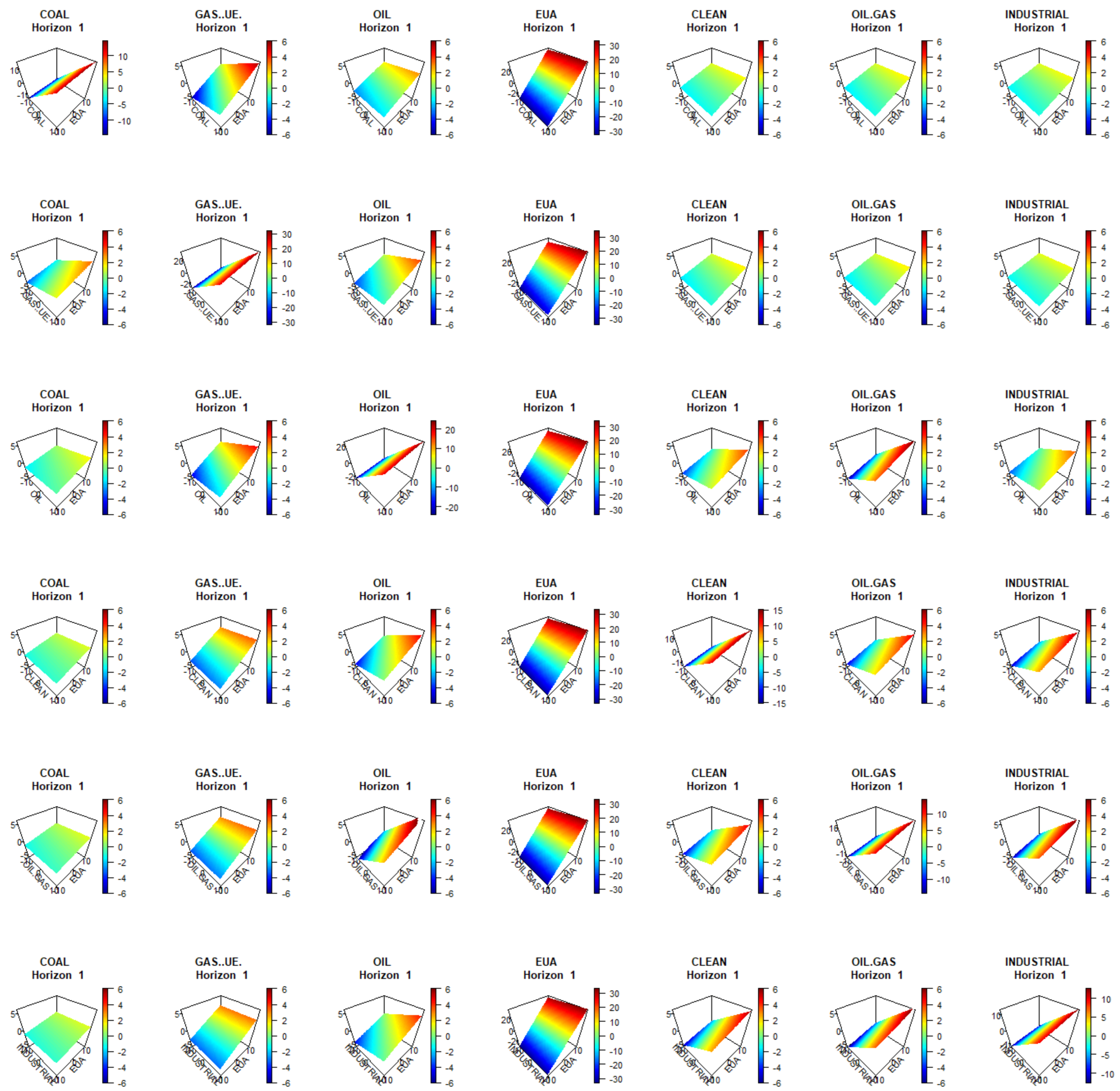
• Impulse response surfaces for conditional mean

Figure 9 shows a 6 × 7 matrix graphic with the response surfaces (in this case planes) of the one step ahead (horizon 1) conditional mean of all of the seven variables (by column and listed on the title of each graph) to bivariate impulses in all pairs of combinations of each variable with EUA (by row). For instance, graphic (1, 2) shows the return response of GAS.UE (axis OZ) to simultaneous shocks in COAL (axis OY) and EUA (axis OX). The size of shocks oscillates from −10 to 10 standard deviations of each series (see axis OX and OY), while the increment of the conditional expected return (axis OZ) oscillates from −6% (blue) to 6% (red). In this case, the positive obliquity of the plane indicates that positive (negative) shocks in COAL and EUA produce an increase (decrease) in the expected GAS.UE return. However, shocks of different signs in COAL and EUA tend to offset their effects on the expected GAS.UE return. In addition, the degree of inclination of the plane, with respect to the plane z = 0 is high, which indicates that the size (in absolute terms) of these effects is high. For instance, simultaneous shocks of 10 (−10) standard deviations in COAL and EUA are expected to increase (decrease) the GAS.UE return around 5%.

Figure 9 highlights that the response functions of each series only depend on its own shocks, independent of the size of the EUA shocks (see graphics (1, 1), (2, 2), (3, 3), (4, 5), (5, 6) and (6, 7)). This fact can be appreciated in the color lines of the plane, which are approximately parallel to the OX axis. Analogously, the response of EUA only depends on its own shocks because the color lines of the plane are parallel to the OY axis (see graphics in column 4).

Regarding cross-effects (Regarding cross-effects, i.e., effects of bivariate shocks in EUA and another series on the response of a third series), column 2 shows that GAS.UE is affected by bivariate EUA-COAL and EUA-OIL shocks. However, for the rest of combinations, the response of GAS.UE is only affected by the EUA shock (the color lines of each plane are parallel to OY axis). Column 1 shows that COAL is only weakly affected by bivariate EUA-GAS.UE shocks (see the low inclination of the plane in graphic (1, 2)). OIL is affected to a greater or lesser extent by the interaction of EUA shocks, with the shocks of other series and the effects of EUA being stronger when combined with the fossil fuels and weaker when combined with the stock indices (see column 3). Finally, CLEAN, OIL.GAS and INDUSTRIAL are affected by the interaction of the EUA shocks, with those of the variables in their block, with EUA having less effect (see graphic (i, j) 5 ≤ i ≠ j ≤ 7).

Figure 10 displays a matrix graphic with the response surfaces of the one step ahead (horizon 1) conditional mean of EUA return to bivariate impulses in all pairs of combinations of the rest of the variables (The impulse response functions of two or more steps ahead were insignificant, due to the high mean reversion of all the series and are omitted for the sake of brevity).

The strongest effects on EUA are exerted by interactions of GAS.UE or OIL shocks with the rest (see graphics in columns 1 and 2 and row 2). In all of the cases, the size of the impacts increases with the size of the shocks.

• Impulse response surfaces for the conditional volatility

Figure 11 presents a matrix graphic with the response surfaces of the one step ahead (horizon = 1) conditional volatility of the seven variables (by column) to bivariate impulses in all pair combinations of each variable with EUA (by row). For instance, graphic (1,2) shows the volatility response of GAS.UE (axis OZ) to impulses in COAL (axis OY) and EUA (axis OX). The size of shocks oscillates from −10 to 10 standard deviations of each series (see axis OX and OY), while the increment of the expected conditional volatility (axis OZ) oscillates from −5 units (blue) to 15 units (red). In this case, the largest increase in volatility corresponds to the largest shocks in absolute value with the same sign. The largest decreases correspond to the largest shocks in absolute value but with different signs.

This figure highlights that the response functions of the conditional volatility of each series only depend on its own shocks, independentl of the size of the EUA shocks (the color lines of the surfaces are approximately parallel to axis OX). With respect to the response functions of EUA (column 4 of Figure 11), they depend on their own shocks (color lines are parallel to axis OY) except when they are combined with GAS.UE shocks (see graphic (2, 4)) in which case a weak interaction effect can be observed. According to cross-effects, GAS.UE is only affected weakly by EUA shocks, except when combined with COAL shocks. Finally, CLEAN, OIL.GAS and INDUSTRIAL are also very weakly affected by the interaction of EUA with shocks of them (see graphic (i, j) 5 ≤ i ≠ j ≤ 7).

Figure 12 shows a matrix graphic with the response surfaces of the one step ahead conditional volatility of EUA to bivariate impulses in all pairs of combinations of the rest of the variables.

The strongest effects on EUA are exerted by interactions of GAS.UE shocks with the rest of series (see graphic (1, 1) and graphic (2, j) 1 ≤ j ≤ 4)). The strongest effect corresponds to the interaction of GAS.UE with CLEAN shocks, when shocks of the corresponding series occur with the same magnitude and direction, while there is a decrease when the direction is different.

Figure 13 shows a matrix graphic with the dynamic evolution of response surfaces of the conditional volatility of each variable to bivariate impulses in all pairs of combinations of each variable with EUA, which contain the most important effects. Each row corresponds to the response of each variable and each column to a temporal horizon.

It can be seen that the shape of the impacts surface is maintained over time and decreases as the time horizon grows, although with different speeds that increasingly depend on the persistence variance of each series (see αi + βI from Table 4). For instance, notice the high persistence in GAS.UE (row 2) and the low persistence in INDUSTRIAL (row 7).

• Impulse response surfaces for the conditional correlation

The analysis of the conditional correlation surfaces revealed that the only significant responses were those corresponding to the combination of shocked variables. For this reason, Figure 14 shows a matrix graphic with only the dynamic evolution of response surfaces of the conditional correlation between each pair of variables to their own shocks. For instance, graphic (1, 1) shows the change of the conditional correlation between COAL and GAS.UE (axis OZ) to simultaneous shocks in COAL (axis OY) and GAS.UE (axis OX). The size of shocks oscillates from −10 to 10 standard deviations of each series (see axis OX and OY), while the increment of the expected conditional correlation (axis OZ) oscillates from −1 units (blue) to 1.5 units (red). The profiles of all surfaces are very similar and show that an increase in the correlation is produced when shocks of the corresponding series occur with the same magnitude and direction, while there is a decrease when the direction is different.

Figure 15 shows the dynamic evolution for different horizons of the response surfaces of the conditional correlation between each variable and EUA in a matrix graphic. Each row corresponds to each pair of variables and each column to a temporal horizon. The effects remain almost intact after 10 days but decrease considerably after 25 days and have practically disappeared after 50 days. This decrease depends on the value of a + b (see Table 4), which is the same for each pair of variables.

Once this in-depth analysis of the impulse response functions of conditional mean, volatility and correlation had been carried out, we analyzed the effects of EUA on the returns and the risk of the rest of variables and vice versa.

If we analyze the impulse response functions of conditional mean, i.e., the expected returns of the series, we notice that the impacts of EUA increase and last for one day due to the existence of a strong mean reversion (see row 4 of Figure 6). The most important impacts are exerted on itself and on GAS.UE and OIL Furthermore, the effects of EUA shocks are enhanced by shocks that affect other variables, when they are of the same sign and are offset if they are of a different sign (see Figure 9). Symmetrically, the shocks of these two variables, both individually (see column 4 of Figure 7) and combined with shocks of other variables (see Figure 10), affect the return of the EUA. In this case, the effects last for two days and are positive in the first day and negative in the second, thus reflecting the existence of a corrective effect typical of the stock markets.

If we consider the responses in volatility (i.e., risk), the most significant impacts of the EUA are exerted on its own volatility and on that of the GAS.UE (see row 4 of Figure 7). The existence of an enhancing effect is only observed when combined with a COAL shock (see column 2 of Figure 11). Symmetrically, the most significant effects on the volatility of EUA correspond to GAS.UE shocks both individually (see column 4 of Figure 7) and combined with shocks from other variables (see graphic (2, 4) of Figure 11 and Figure 12). In both cases, the persistence of these effects is high (see row 4 and column 4 of Figure 7 and Figure 13) and their values increase with the absolute value of the impacts.

Finally, taking into account the correlation responses, the most significant impacts on the correlations of the EUA with another variable are exerted by the shocks that affect them. These impacts increase the value of the correlation and, therefore, the possibility of a risk synergy effect between them. This effect is persistent (see row 4 and column 4 of Figure 8 and Figure 15) and is bigger, the greater the absolute value of the shock. Furthermore, this effect is enhanced if shocks of the same sign are produced simultaneously in both variables (see Figure 15).

4.3. Optimal Portfolio Weights

The importance of identifying the spillover effect of volatility and correlation in a dynamic way is crucial to efficiently managing investment portfolios and to carrying out optimal diversification of assets. This intelligent management allows for reducing the risk and controlling the changes that may occur, due to the economic situation in general or greater restrictions with the mechanisms that adjust the supply of allowances.

In this section, we use the results of the estimated VAR(1)-DCC(1,1)-GARCH(1,1) model in Section 4.1 to investigate portfolio diversification opportunities amongst different alternative energy financial markets. For this aim, and given that most of investors are risk averse and prefer less risk for the same level of expected return [54], we will focus on risk reduction and Markowitz’s minimum variance portfolios. Their weights are obtained sequentially, by minimizing the volatility of the portfolio subject to a required return constraint. This problem can be formulated as:

$$\begin{gathered} \underset{{\mathsf{\omega }}_{\mathrm{t}}}{\min } {\mathsf{\omega }}_{\mathrm{t}}^{\prime }{H}_{\mathrm{t}}{\mathsf{\omega }}_{\mathrm{t}} \\ \mathrm{s}.\mathrm{t}. {\mathsf{\omega }}_{\mathrm{t}}^{\prime }\mathsf{\mu }=1 \end{gathered}$$

where ${\mathsf{\omega }}_{\mathrm{t}}={\left({\mathsf{\omega }}_{1,\mathrm{t}},\dots ,{\mathsf{\omega }}_{\mathrm{N},\mathrm{t}}\right)}^{\prime }$ is the vector of portfolio weights for time t chosen at time t − 1, H_t is the conditional variance and covariance matrix of a vector of returns for time t and µ is the assumed vector of returns. The solution to this problem is:

$${\mathsf{\omega }}_{\mathrm{t}}=\frac{H_{\mathrm{t}}^{-1}\mathsf{\mu }}{{\mathsf{\mu }}^{\prime }{H}_{\mathrm{t}}^{-1}\mathsf{\mu }}$$

(1)

Note that ${{\displaystyle \sum }}_{\mathrm{i}=1}^{\mathrm{N}}{\mathsf{\omega }}_{\mathrm{i},\mathrm{t}}$, with ${\omega }_{i,t}$ being the share on asset i for time t, generally will not need to be equal to 1. Indeed, 1$-{{\displaystyle \sum }}_{\mathrm{i}=1}^{\mathrm{n}}{\mathsf{\omega }}_{\mathrm{i},\mathrm{t}}$ is the share in the risk-free asset.

This optimal portfolio selection procedure assigns greater weight to assets with high-expected return and low expected variance, and vice versa. As on the one hand, investors with different expected returns will hold different portfolios and, on the other hand, it is impossible to know the true vector of expected returns, we will carry out the optimization process for a wide range of hypothetical time-invariant vectors of expected returns, which are not required to be the true one. Different investors at different times have different vectors of expected returns; therefore, we take a set of return vectors capturing possible and different scenarios, where returns could be high, and others in which they could be low or even zero. Asset pricing theory suggests that the unconditional expected returns for stocks should be positive, and that stocks should have the highest expected return. So, following [55,56,57], we do not consider return vectors with all of their components negative, because this does not respond to reality. The selected vectors of returns have to be a proxy of expected returns, and the prior belief of investors is that those returns should be non-negative, and even as high as possible. Once we select that set of return vectors, we can calculate the corresponding weights for each of them by applying (1), and consequently we obtain the optimal portfolio. The last step of the selecting process of the final optimal portfolio is to take the weight for each of its assets and the average of the weights obtained in the different optimal portfolios for each return vectors of the considered set.

With this way of acting, in our particular case, we have followed three different strategies to determine the set of return vectors. In the first case, we take the no overlapping 134 monthly averages of the observed returns included in the analyzed period, and we discard five vectors whose components are all negative. In the second case, we calculate the no overlapping 45 quarterly averages included in our period, discarding two vectors in which all of their components are negative. Finally, in the third case, we have considered the no overlapping 13 yearly averages without discarding any. In order to compare and select the best option of the three strategies we follow the approach of [56].

Table 5. Diebold and Mariano test with heteroscedasticity correction.

	Monthly	Quarterly	Yearly
Monthly		2.2707	−2.1427
Quarterly	−2.2707		−2.5858
Yearly	2.1427	2.5858

All the results are significant at 5%.

provides the t-statistics of the Diebold–Mariano test (see details in the Appendix A) to compare the volatilities of two dynamic portfolios. The null hypothesis of this test is that there is no difference between the portfolio variances. In our case, we have compared the portfolios selected by the three strategies (monthly, quarterly and annually) described earlier. The t-statistics provided in the table are the result of comparing the strategy in the column with the one in the row. A negative (positive) value of the t statistic is evidence in favor of better (worse) performance, in terms of volatilities, of the row strategy. We can observe that the strategy with a statistically significant risk reduction is the second one, corresponding to that obtained with the 43 quarterly return averages.

In addition, Figure 16 displays in a two-panel graphic the evolution of the daily portfolio volatility (left panel) and the daily evolution of the portfolio return (right panel) obtained with the three strategies (red lines correspond to the monthly strategy, black lines to the quarterly strategy and blue lines to the yearly strategy). The volatilities pattern (left panel) is similar in the three strategies, but the oscillations are clearly greater in the yearly average strategy and smaller in the quarterly one, causing the Diebold and Mariano test to select this latter strategy as the best. The profile in the three volatility lines indicates that there are two periods of high volatility, which correspond to April 2013 and March 2020. The maximum in April 2013 corresponds to the onset of phase III with a change in the allocations of allowances and the regularization of the EU ETS because there was a surplus of allowances due to the economic crisis. The EUA price fell from 4.71 to 3.1 and the on following day to 2.5; therefore, in total, it had a drop of more than 50%, which caused high volatility, which is reflected in the composition of the portfolio. The second most important peak corresponds to March 2020 and coincides with the declaration of the health crisis due to the COVID-19 pandemic, which unleashed a great storm in the markets, producing high volatility (see Figure 5). With respect to the right panel of Figure 16, which displays the daily evolution of the portfolio return, we can observe a more homogeneous behavior in the oscillation levels of returns throughout time than in the case of individual assets (see Figure 2), which shows a higher control of the inversion risk.

Figure 17 shows only the evolution of the weights of the optimal portfolio corresponding to the quarterly strategy. The message obtained from the other two strategies (monthly and annual) is very similar and they are not shown for the sake of brevity.

The analysis of the optimal weights shows how the clean energy sector has become important in optimal diversification strategies with the passage of time. Clearly, CLEAN is the asset with the greatest weight in the portfolio 74.72% of the days, followed by EUA with 7.74%. Therefore, it is clear that clean energies have been playing a relevant role in recent years. To diversify the risks, the portfolio has to go short on selling OIL.GAS asset on 91.47% of the days. This is due to those assets tending to have lower volatility levels throughout the analyzed period. Raw materials have specific moments in which they have the largest weights: COAL has been 5.83%, GAS.UE, 7.52% and OIL 3.18%. All of the EUA weights were positive with intermediate values, between 8% and 35%, due to its higher levels of volatility.

It is observed that the weight in CLEAN was the largest from the end of 2016 to February 2020, where it fell due to the pandemic. The closure of most thermal power plants at the beginning of 2020 caused a sharp fall in the price of COAL, which may explain the increase in its weight in the portfolio in the first quarter of 2020. We can see that the weight of OIL was below CLEAN since 2017, but the COVID 2019 crisis has caused interest in renewable energies to be lost and OIL has become important again. This fact could be due to markets taking the economic recovery for granted. The derivative markets, in which raw materials, such as oil are traded, move with expectations, and these are of economic reactivation due to medical advances and vaccination processes. The COVID-19 vaccine is promoting better forecasts for the economy, in which the rise in fuel prices plays an important role. When dealing with expectations, investors believe that these prices will continue to rise until a real balance between supply and demand is produced.

5. Conclusions

This paper has carried out a dynamic multivariate study of the evolution of return of financial assets, related to the energy market (fossil fuels, energy companies and industrial firms). For this, the VAR-DCC-GARCH family of models has been used, which provides a very adequate framework to describe their joint evolution, taking into account their heteroscedastic nature, as well as the temporal evolution of the variances and the correlations between these series. This allows, on the one hand, analysis of the impulse response functions of these moments before unexpected shocks affecting each series and, on the other hand, to capture the patterns existing in the joint evolution of the series in terms of the binomial risk-return, which constitutes crucial information for the design of investment portfolios. In particular, special attention has been paid to the temporal evolution of the prices of the CO₂ European Emission Allowances, in order to know if these prices are helping to achieve the objective of encouraging the use of renewable energy and reducing that of dirty energy so that the EU can meet climate objectives.

Our results show the existence of three groups of assets with little influence on each other. One group is made up of COAL and GAS.UE, a second block is OIL and the stock indices of energy and industrial companies and, lastly, a third block with only the allowance prices. The first two groups tend to move simultaneously in the same direction with significantly positive correlations, and with high persistence in volatility. While it is true that the correlations change over time, they fluctuate relatively little around an average value, and also reflect high persistence.

Regarding the return of CO₂ allowances, its correlation is positive with all the returns series, although this is not very strong. The most important impacts of the EUA shocks on the expected returns and the risk are exerted on itself and on GAS.UE, and vice versa. The impact on mean lasts at most two days, and they are enhanced by shocks that affect other variables when they are of the same sign, and are offset if they are of a different sign. The persistence of the impacts on volatility is high and an enhancing effect of the EUA on GAS.UE is only observed when combined with a COAL shock, while this pushing up effect occurs on EUA if the GAS.UE shock is combined with shocks from other variables. Finally, the most significant impacts on the correlations of the EUA with another variable are exerted by the shocks that affect them. These impacts increase the value of the correlation and, therefore, the possibility of a risk synergy effect between them. This effect is persistent and is bigger, the greater the absolute value of the shock. Furthermore, this effect is enhanced if shocks of the same sign are produced simultaneously in both variables.

In terms of investment, this paper has dynamically calculated the composition of a portfolio, with minimal volatility and required return of assets related to fossil fuels, allowances and energy companies. The results show the importance of investing in clean companies, due to their lower volatility, while also offsetting the risk with short investments in oil and gas companies due to their lower volatility. These weights increase significantly in economic boom years, in which clean companies tend to be an asset to be taken into account, due to their low levels of volatility and increased return. In times of crisis, however, its weighting falls in favor of fossil fuels and allowances. All of this achieves returns with more homogeneous oscillation levels, only altered by unexpected situations, such as, for example, the current pandemic, which has significantly increased the levels of uncertainty in all of the series analyzed.

Although, from the speculation point of view, investing in the EUA does not play a relevant role, but an indirect influence in favor of the environment is observed, which is highlighted with the growth of the weights of clean energy assets in the optimal portfolio with time. This result highlights the declining of dirty energies and the rising of the clean energy market, also amongst the investment community, which might be an indication of the progress towards the energy transition to renewables sources, within a circular economy perspective. Therefore, this shows that the EU ETS is achieving its goals and that clean energy companies, aligned with their role towards socially responsible initiatives, could also gain acceptance in terms of investments, which would be beneficial for the environment.

From our point of view, the information provided by our results may be useful for policymakers (European commission) when evaluating the impact that the restrictions imposed on the carbon market by the MSR have had on investment in assets of energy and industrial companies. In addition, our results could make investments in green and clean energy assets more appealing to investors, which indirectly have positive implications regarding social and economic development. Therefore, this could affect the welfare of clean and green investments, given the evidence on the utility of these renewable energy investments in mitigating the downside risk of their competent and counterpart dirty energy assets.

Despite our good results, it would be interesting to carry out an economic valuation of the volatility in this field, suggested by [55,56]. This future research would take into account more general MGARCH models and the risk aversion of the investor. Additionally, it could be interesting to extend our results by investigating the dynamic directional information spillover of return and volatility between the four markets: fossil fuels, energy, industrial stocks and EUA in line with [58].

References

1. Ellerman, A.D. New entrant and closure provisions: How do they distort? Energy J. 2008, 29. [Google Scholar] [CrossRef] [Green Version]
2. Ellerman, D.; Convery, F.; De Perthuis, C. The European carbon market in action: Lessons from the first trading period. J. Eur. Environ. Plan. Law 2008, 5, 215–233. [Google Scholar] [CrossRef] [Green Version]
3. Parsons, J.E.; Feilhauer, S.; Ellerman, A.D. Designing a U.S. market for CO2. J. Appl. Corp. Financ. 2009, 21, 79–86. [Google Scholar] [CrossRef]
4. Hu, J.; Crijns-Graus, W.; Lam, L.; Gilbert, A. Ex-ante evaluation of EU ETS during 2013–2030: EU-internal abatement. Energy Policy 2015, 77, 152–163. [Google Scholar] [CrossRef]
5. Dhamija, A.K.; Yadav, S.S.; Jain, P. Volatility spillover of energy markets into EUA markets under EU ETS: A multi-phase study. Environ. Econ. Policy Stud. 2017, 20, 561–591. [Google Scholar] [CrossRef]
6. Jiménez-Rodríguez, R. What happens to the relationship between EU allowances prices and stock market indices in Europe? Energy Econ. 2019, 81, 13–24. [Google Scholar] [CrossRef]
7. Chèze, B.; Chevallier, J.; Berghmans, N.; Alberola, E. On the CO2 emissions determinants during the EU ETS phases I and II: A plant-level analysis merging the EUTL and Platts power data. Energy J. 2020, 41. [Google Scholar] [CrossRef]
8. Uddin, G.S.; Hernandez, J.A.; Shahzad, S.J.H.; Hedström, A. Multivariate dependence and spillover effects across energy commodities and diversification potentials of carbon assets. Energy Econ. 2018, 71, 35–46. [Google Scholar] [CrossRef]
9. Lamphiere, M.; Blackledge, J.; Kearney, D. Carbon futures trading and short-term price prediction: An analysis using the fractal market hypothesis and evolutionary computing. Mathematics 2021, 9, 1005. [Google Scholar] [CrossRef]
10. Rockström, J.; Steffen, W.; Noone, K.; Persson, Å.; Chapin, F.S.I.; Lambin, E.; Lenton, T.M.; Scheffer, M.; Folke, C.; Schellnhuber, H.J.; et al. Planetary boundaries: Exploring the safe operating space for humanity. Ecol. Soc. 2009, 14, 1–33. [Google Scholar] [CrossRef]
11. Jones, C.M.; Kaul, G. Oil and the stock markets. J. Financ. 1996, 51, 463–491. [Google Scholar] [CrossRef]
12. Park, J.; Ratti, R.A. Oil price shocks and stock markets in the U.S. and 13 European countries. Energy Econ. 2008, 30, 2587–2608. [Google Scholar] [CrossRef]
13. Kilian, L.; Park, C. The impact of oil price shocks on the U.S. stock market. Int. Econ. Rev. 2009, 50, 1267–1287. [Google Scholar] [CrossRef]
14. Managi, S.; Okimoto, T. Does the price of oil interact with clean energy prices in the stock market? Jpn. World Econ. 2013, 27, 1–9. [Google Scholar] [CrossRef] [Green Version]
15. Kumar, S.; Managi, S.; Matsuda, A. Stock prices of clean energy firms, oil and carbon markets: A vector autoregressive analysis. Energy Econ. 2012, 34, 215–226. [Google Scholar] [CrossRef]
16. Gallego-Álvarez, I.; Segura, L.; Martinez-Ferrero, J. Carbon emission reduction: The impact on the financial and operational performance of international companies. J. Clean. Prod. 2015, 103, 149–159. [Google Scholar] [CrossRef]
17. Dutta, A.; Bouri, E.; Noor, H. Return and volatility linkages between CO2 emission and clean energy stock prices. Energy 2018, 164, 803–810. [Google Scholar] [CrossRef]
18. Zhang, Y.-J.; Wei, Y.-M. An overview of current research on EU ETS: Evidence from its operating mechanism and economic effect. Appl. Energy 2010, 87, 1804–1814. [Google Scholar] [CrossRef]
19. Subramaniam, N.; Wahyuni, D.; Cooper, B.J.; Leung, P.; Wines, G. Integration of carbon risks and opportunities in enterprise risk management systems: Evidence from Australian firms. J. Clean. Prod. 2015, 96, 407–417. [Google Scholar] [CrossRef]
20. Zhang, Y.-J.; Sun, Y.-F. The dynamic volatility spillover between European carbon trading market and fossil energy market. J. Clean. Prod. 2016, 112, 2654–2663. [Google Scholar] [CrossRef]
21. Wang, Y.; Guo, Z. The dynamic spillover between carbon and energy markets: New evidence. Energy 2018, 149, 24–33. [Google Scholar] [CrossRef]
22. Lin, B.; Chen, Y. Dynamic linkages and spillover effects between CET market, coal market and stock market of new energy companies: A case of Beijing CET market in China. Energy 2019, 172, 1198–1210. [Google Scholar] [CrossRef]
23. Xia, T.; Ji, Q.; Zhang, D.; Han, J. Asymmetric and extreme influence of energy price changes on renewable energy stock performance. J. Clean. Prod. 2019, 241, 118338. [Google Scholar] [CrossRef]
24. Chevallier, J. A model of carbon price interactions with macroeconomic and energy dynamics. Energy Econ. 2011, 33, 1295–1312. [Google Scholar] [CrossRef]
25. Castagneto-Gissey, G. How competitive are EU electricity markets? An assessment of ETS phase II. Energy Policy 2014, 73, 278–297. [Google Scholar] [CrossRef]
26. Hammoudeh, S.; Nguyen, D.K.; Sousa, R. Energy prices and CO2 emission allowance prices: A quantile regression approach. Energy Policy 2014, 70, 201–206. [Google Scholar] [CrossRef] [Green Version]
27. Hammoudeh, S.; Lahiani, A.; Nguyen, D.K.; Sousa, R. An empirical analysis of energy cost pass-through to CO2 emission prices. Energy Econ. 2015, 49, 149–156. [Google Scholar] [CrossRef]
28. Chevallier, J.; Nguyen, D.K.; Reboredo, J.C. A conditional dependence approach to CO2-energy price relationships. Energy Econ. 2019, 81, 812–821. [Google Scholar] [CrossRef]
29. Liu, H.-H.; Chen, Y.-C. A study on the volatility spillovers, long memory effects and interactions between carbon and energy markets: The impacts of extreme weather. Econ. Model. 2013, 35, 840–855. [Google Scholar] [CrossRef]
30. Marimoutou, V.; Soury, M. Energy markets and CO2 emissions: Analysis by stochastic copula autoregressive model. Energy 2015, 88, 417–429. [Google Scholar] [CrossRef]
31. Filis, G. Macro economy, stock market and oil prices: Do meaningful relationships exist among their cyclical fluctuations? Energy Econ. 2010, 32, 877–886. [Google Scholar] [CrossRef]
32. Choi, K.; Hammoudeh, S. Volatility behavior of oil, industrial commodity and stock markets in a regime-switching environment. Energy Policy 2010, 38, 4388–4399. [Google Scholar] [CrossRef]
33. Broadstock, D.C.; Cao, H.; Zhang, D. Oil shocks and their impact on energy related stocks in China. Energy Econ. 2012, 34, 1888–1895. [Google Scholar] [CrossRef] [Green Version]
34. Antonakakis, N.; Filis, G. Oil prices and stock market correlation: A time-varying approach. Int. J. Energy Stat. 2013, 1, 17–29. [Google Scholar] [CrossRef]
35. Henriques, I.; Sadorsky, P. Oil prices and the stock prices of alternative energy companies. Energy Econ. 2008, 30, 998–1010. [Google Scholar] [CrossRef]
36. Sadorsky, P. Correlations and volatility spillovers between oil prices and the stock prices of clean energy and technology companies. Energy Econ. 2012, 34, 248–255. [Google Scholar] [CrossRef]
37. Bondia, R.; Ghosh, S.; Kanjilal, K.; Bondia, R.; Ghosh, S.; Kanjilal, K. International crude oil prices and the stock prices of clean energy and technology companies: Evidence from non-linear cointegration tests with unknown structural breaks. Energy 2016, 101, 558–565. [Google Scholar] [CrossRef]
38. Reboredo, J.C. Is there dependence and systemic risk between oil and renewable energy stock prices? Energy Econ. 2015, 48, 32–45. [Google Scholar] [CrossRef]
39. Ji, Q.; Zhang, D.; Geng, J.-B. Information linkage, dynamic spillovers in prices and volatility between the carbon and energy markets. J. Clean. Prod. 2018, 198, 972–978. [Google Scholar] [CrossRef]
40. Oberndorfer, U. EU emission allowances and the stock market: Evidence from the electricity industry. Ecol. Econ. 2009, 68, 1116–1126. [Google Scholar] [CrossRef] [Green Version]
41. Bushnell, J.B.; Chong, H.; Mansur, E.T. Profiting from regulation: Evidence from the European carbon market. Am. Econ. J. Econ. Policy 2013, 5, 78–106. [Google Scholar] [CrossRef]
42. Jong, T.; Couwenberg, O.; Woerdman, E. Does EU emissions trading bite? An event study. Energy Policy 2014, 69, 510–519. [Google Scholar] [CrossRef] [Green Version]
43. Oestreich, A.M.; Tsiakas, I. Carbon emissions and stock returns: Evidence from the EU emissions trading scheme. J. Bank. Financ. 2015, 58, 294–308. [Google Scholar] [CrossRef]
44. Moreno, B.; Da Silva, P.P. How do Spanish polluting sectors’ stock market returns react to European Union allowances prices? A panel data approach. Energy 2016, 103, 240–250. [Google Scholar] [CrossRef]
45. Tian, Y.; Akimov, A.; Roca, E.; Wong, V. Does the carbon market help or hurt the stock price of electricity companies? Further evidence from the European context. J. Clean. Prod. 2016, 112, 1619–1626. [Google Scholar] [CrossRef] [Green Version]
46. Ji, Q.; Xia, T.; Liu, F.; Xu, J.-H. The information spillover between carbon price and power sector returns: Evidence from the major European electricity companies. J. Clean. Prod. 2019, 208, 1178–1187. [Google Scholar] [CrossRef]
47. Ma, Y.; Wang, L.; Zhang, T. Research on the dynamic linkage among the carbon emission trading, energy and capital markets. J. Clean. Prod. 2020, 272, 122717. [Google Scholar] [CrossRef]
48. Engle, R. Dynamic conditional correlation. J. Bus. Econ. Stat. 2002, 20, 339–350. [Google Scholar] [CrossRef]
49. Tse, Y.K.; Tsui, A.K.C. A multivariate generalized autoregressive conditional heteroscedasticity model with time-varying correlations. J. Bus. Econ. Stat. 2002, 20, 351–362. [Google Scholar] [CrossRef]
50. Engle, R.; Sheppard, K. Theoretical and Empirical Properties of Dynamic Conditional Correlation Multivariate GARCH; National Bureau of Economic Research: Cambridge, MA, USA, 2001; p. 8554. [Google Scholar]
51. Hafner, C.M.; Herwartz, H. Volatility impulse responses for multivariate GARCH models: An exchange rate illustration. J. Int. Money Financ. 2006, 25, 719–740. [Google Scholar] [CrossRef]
52. Sharpe, W.F.; Alexander, G.J.; Bailey, J.V. Investments, 6th ed.; Prentice Hall: Upper Saddler River, NJ, USA, 1999; ISBN 978-0-13-010130-3. [Google Scholar]
53. Tsay, R.S. An Introduction to Analysis of Financial Data with R; Wiley and Sons: Hoboken, NJ, USA, 2013; ISBN 978-0-470-89081-3. [Google Scholar]
54. Fleming, J.; Kirby, C.; Ostdiek, B. The economic value of volatility timing using “realized” volatility. J. Financ. Econ. 2003, 67, 473–509. [Google Scholar] [CrossRef]
55. Engle, R.; Colacito, R. Testing and valuing dynamic correlations for asset allocation. J. Bus. Econ. Stat. 2006, 24, 238–253. [Google Scholar] [CrossRef]
56. Dichtl, H.; Drobetz, W.; Wendt, V. How to build a factor portfolio: Does the allocation strategy matter? Eur. Financ. Manag. 2020, 27, 20–58. [Google Scholar] [CrossRef]
57. Diebold, F.X.; Mariano, R.S. Comparing predictive accuracy. J. Bus. Econ. Stat. 2002, 20, 134–144. [Google Scholar] [CrossRef]
58. Song, Y.; Ji, Q.; Du, Y.-J.; Geng, J.-B. The dynamic dependence of fossil energy, investor sentiment and renewable energy stock markets. Energy Econ. 2019, 84, 104564. [Google Scholar] [CrossRef]
Figure 1. Matrix graph with the evolution of the daily prices of the seven series.
Mathematics 09 01787 g001
Figure 2. Matrix graph with the evolution of the daily returns of the seven series.
Mathematics 09 01787 g002
Figure 3. Cross-correlation function of the returns of the seven series in the off-diagonal cells and with the autocorrelation function on themselves in the diagonal.
Mathematics 09 01787 g003
Figure 4. Matrix graph with the cross-correlation function of the residuals of the VAR(1) model in the off-diagonal cells, and with the autocorrelation function of the quadratic residuals in the diagonal.
Mathematics 09 01787 g004
Figure 5. Matrix graph with the estimated dynamic correlation between two variables in the off-diagonal cells and with the estimated volatility of the daily returns of the seven series in the diagonal. The estimated constant correlation of a VAR(1)-CCC-GARCH(1,1) model is in red.
Mathematics 09 01787 g005
Figure 6. Matrix graph with the mean impulse response curves for several forecast horizons and shock sizes. The off-diagonal cells contain the response of the conditional mean of one variable, when the shocked variable is a different one and the diagonal cells encloses the responses when the shocks are produced on itself (the shocked variable in brackets).
Mathematics 09 01787 g006
Figure 7. Matrix graph with the volatility impulse response curves for several forecast horizons and shock sizes. The off-diagonal cells contain the response of the conditional volatility of one variable when the shocked variable is a different one and the diagonal cells enclose the responses when the shocks are produced on itself (the shocked variable in brackets).
Mathematics 09 01787 g007
Figure 8. Matrix graph with the conditional correlation impulse response curves for several forecast horizons and shock sizes. The off-diagonal cells of each row contain the response of the correlation between the shocked variable and each of the others. The diagonal cells specify the shocked variable.
Mathematics 09 01787 g008
Figure 9. Matrix graph with the response surfaces of the conditional mean of all of the seven variables (by column) to bivariate impulses in all pairs of combinations of each variable with EUA (by row).
Mathematics 09 01787 g009
Figure 10. Matrix graph with the response surfaces of the conditional mean of EUA to bivariate impulses in all pairs of combinations of the rest of the variables.
Mathematics 09 01787 g010
Figure 11. Matrix graph with the response surfaces of the conditional volatility of all of the seven variables (by column) to bivariate impulses in all pair combinations of each variable with EUA (by row).
Mathematics 09 01787 g011
Figure 12. Matrix graph with the response surfaces of the conditional volatility of EUA to bivariate impulses in all pairs of combinations of the rest of the variables.
Mathematics 09 01787 g012
Figure 13. Matrix graph with the dynamic evolution of response surfaces of the conditional volatility of each variable to bivariate impulses in all pairs of combinations of each variable with EUA. Each row corresponds to the response of each variable and each column to a temporal horizon.
Mathematics 09 01787 g013
Figure 14. Matrix graph with the response surfaces of the conditional correlation between all pairs of combinations of two variables to bivariate impulses on themselves.
Mathematics 09 01787 g014
Figure 15. Matrix graph with the dynamic evolution of response surfaces of the conditional correlation between each variable and EUA to bivariate impulses of different size on themselves. Each row corresponds to each pair of variables and each column to a temporal horizon.
Mathematics 09 01787 g015
Figure 16. Evolution of the daily portfolio volatility (left panel) and of the daily portfolio return (right panel) for the three strategies (monthly in red line, quarterly in black line and yearly in blue line).
Mathematics 09 01787 g016
Figure 17. Evolution of the weights of the optimal portfolio composed by fossil fuels, energy stocks, EU allowances and a risk-free asset.
Mathematics 09 01787 g017