Collocation Methods for High-Order Well-Balanced Methods for Systems of Balance Laws

Abstract

In some previous works, two of the authors introduced a technique to design high-order numerical methods for one-dimensional balance laws that preserve all their stationary solutions. The basis of these methods is a well-balanced reconstruction operator. Moreover, they introduced a procedure to modify any standard reconstruction operator, like MUSCL, ENO, CWENO, etc., in order to be well-balanced. This strategy involves a non-linear problem at every cell at every time step that consists in finding the stationary solution whose average is the given cell value. In a recent paper, a fully well-balanced method is presented where the non-linear problems to be solved in the reconstruction procedure are interpreted as control problems. The goal of this paper is to introduce a new technique to solve these local non-linear problems based on the application of the collocation RK methods. Special care is put to analyze the effects of computing the averages and the source terms using quadrature formulas. A general technique which allows us to deal with resonant problems is also introduced. To check the efficiency of the methods and their well-balance property, they have been applied to a number of tests, ranging from easy academic systems of balance laws consisting of Burgers equation with some non-linear source terms to the shallow water equations—without and with Manning friction—or Euler equations of gas dynamics with gravity effects.

1. Introduction

Let us consider a PDE system of the form:

$$U_t(x,t)+f{\left(U(x,t)\right)}_x=S\left(U(x,t)\right)H_x\left(x\right),x\in \mathbb{R},t>0,$$

(1)

where $U(x,t)$ takes values on an open convex set $\mathsf{\Omega }\subset {\mathbb{R}}^N$, $f:\mathsf{\Omega }⟶{\mathbb{R}}^N$ is the flux function, $S:\mathsf{\Omega }⟶{\mathbb{R}}^N$, and H is a continuous known function from $\mathbb{R}$ to $\mathbb{R}$ (possibly the identity function $H\left(x\right)=x$). It is supposed that system (1) is strictly hyperbolic, that is, ${\displaystyle D_f\left(U\right)=\frac{\partial f}{\partial U}\left(U\right)}$ has N real distinct eigenvalues $r_1\left(U\right),\dots ,r_N\left(U\right)$ and associated eigenvectors $v_1,\dots ,v_N$.

Systems of the form (1) have non-trivial stationary solutions that satisfy the ODE system:

$$f{\left(U\right)}_x=S\left(U\right)H_x.$$

(2)

A numerical method is said to be well-balanced if it has discrete stationary solutions that approximate all the stationary solutions of the system or, at least, a relevant family of them. The design of numerical methods that have the previous property is of great importance in problems where small perturbations of a stationary solution are going to be considered, like in many geophysical problems. Methods that are well-balanced have been proposed by many authors: for example, References [1,2,3,4,5,6,7,8,9,10,11,12,13,14,15,16,17,18,19,20,21,22,23,24,25,26,27,28,29,30,31,32,33,34,35] and their references.

The aim of this work is to introduce a general methodology to build well-balanced high-order finite-volume numerical methods for (1) of the form:

$$\frac{d{\tilde{U}}_i}{dt}=-\frac{1}{\mathsf{\Delta }x}\left(F_{i+\frac{1}{2}}\left(t\right)-F_{i-\frac{1}{2}}\left(t\right)\right)+\frac{1}{\mathsf{\Delta }x}{S}_i,$$

(3)

where:

• $I_i=\left[x_{i-\frac{1}{2}},x_{i+\frac{1}{2}}\right]$ are the computational cells, whose length $\mathsf{\Delta }x$ is supposed to be constant for simplicity;
• ${\tilde{U}}_i\left(t\right)$ is the approximation of the average of the exact solution at the ith cell at time t, that is,

  $${\tilde{U}}_i\left(t\right)\cong \frac{1}{\mathsf{\Delta }x}{\int }_{x_{i-\frac{1}{2}}}^{x_{i+\frac{1}{2}}}U(x,t)dx;$$
• $F_{i+\frac{1}{2}}=\mathbb{F}(U_{i+\frac{1}{2}}^{t,-},U_{i+\frac{1}{2}}^{t,+})$, where $\mathbb{F}$ is a consistent numerical flux, and $U_{i+\frac{1}{2}}^{t,\pm }$ are the reconstructed states at the intercells, i.e.,

  $$U_{i+\frac{1}{2}}^{t,-}=P_i^t\left(x_{i+\frac{1}{2}}\right),U_{i+\frac{1}{2}}^{t,+}=P_{i+1}^t\left(x_{i+\frac{1}{2}}\right),$$

  where $P_i^t\left(x\right)$ is a reconstruction of order p of the solution at the given ith cell, computed from the sequence $\left\{{\tilde{U}}_i\left(t\right)\right\}$:

  $$P_i^t\left(x\right)=P_i(x;{\left\{{\tilde{U}}_j\left(t\right)\right\}}_{j\in S_i}),$$

  where $S_i$ is the set of cell indices belonging to the stencil associated to $P_i^t\left(x\right)$;
• finally,

  $$S_i\approx {\int }_{x_{i-\frac{1}{2}}}^{x_{i+\frac{1}{2}}}S\left(P_i^t\left(x\right)\right)H_x\left(x\right)dx.$$

  (4)

Given a function U, the following notation will be used to represent its cell averages and the approximations to its cell averages or its point values at the intercells:

$${\overline{U}}_i=\frac{1}{\mathsf{\Delta }x}{\int }_{x_{i-1/2}}^{x_{i+1/2}}U\left(x\right)dx,{\tilde{U}}_i\approx {\overline{U}}_i,U^{i+1/2}\approx U\left(x_{i+1/2}\right),\forall i.$$

Following References [36,37], the well-balanced property of the methods can be transferred to the reconstruction operator:

Definition 1.

A reconstruction operator $P_i\left(x\right)$ is said to be well-balanced for a function $U^{*}$ if

$$P_i\left(x\right)=U^{*}\left(x\right),\forall x\in [x_{i-\frac{1}{2}},x_{i+\frac{1}{2}}],\forall i,$$

(5)

where $P_i$ is the approximation of $U^{*}$ computed from the vector of cell-averages $\left\{{\overline{U}}_i^{*}\right\}$ of the function $U^{*}$.

In Reference [37], it has been proved that the numerical method (3) is exactly well-balanced according to Definition 2 if the reconstruction operator is well-balanced for every stationary solution $U^{*}$ and

$$S_i={\int }_{x_{i-\frac{1}{2}}}^{x_{i+\frac{1}{2}}}S\left(P_i^t\left(x\right)\right)H_x\left(x\right)dx.$$

(6)

Definition 2.

The numerical method (3) is said to be exactly well-balanced if the sequence of cell-averages $\left\{{\overline{U}}_i^{*}\right\}$ (or the sequence of their approximations $\left\{{\tilde{U}}_i^{*}\right\}$ if a quadrature formula is used to compute them) of any stationary solution $U^{*}$ of (1) is an equilibrium of the ODE system (3).

Furthermore, in References [36,37], the authors propose a method to build a well-balanced reconstruction operator from any standard one that will be recalled in the next section. As we shall see, the main difficulty in the application of this technique comes from the fact that, at every cell and at every time step, one has to solve a non-linear problem of the form:

Find U such that

$$\left\{\begin{array}{c}{\displaystyle f{\left(U\right)}_x=S\left(U\right)H_x,}\hfill \\ {\displaystyle \frac{1}{{\Delta }x}{\int }_{x_{i-1/2}}^{x_{i+1/2}}U\left(x\right)dx={\tilde{U}}_i,}\hfill \end{array}\right.$$

(7)

where ${\tilde{U}}_i$ is an approximation of the average at the i-th cell of the sought solution of (1). Once this problem with given average has been solved at the cell, the solution of (7), that will be denoted by $U_i^{*}$, has to be extended to the whole stencil by solving two Cauchy problems of the form

$$\left\{\begin{array}{c}{\displaystyle f{\left(U\right)}_x=S\left(U\right)H_x,}\hfill \\ U\left(x_{i+1/2}\right)=U^{i+1/2}.\hfill \end{array}\right.$$

(8)

More precisely, (8) with initial condition $U\left(x_{i+1/2}\right)=U^{*}\left(x_{i+1/2}\right)$ (resp. with final condition $U\left(x_{i-1/2}\right)=U^{*}\left(x_{i-1/2}\right)$ ) has to be solved forward in space (resp. backward in space) in the cells at the right (resp. at the left) of the ith cell in its stencil.

The previous procedure has been applied to balance laws whose stationary solutions are known in implicit or explicit form, so that problems (7) and (8) can be easily solved: see, for example, References [32,38], and the references therein. However, when solving these problems by analytic procedures is not possible, they have to be solved numerically. Please note that the two main difficulties come from the condition on the average in (7) and from the fact that the ODE is not in normal form: special care has to be taken in resonant problems i.e., problems in which the Jacobian matrix of the flux, $D_f\left(U\right)$ becomes singular. When the Jacobian is regular, the ODE system (2) can be written in normal form

$$U_x=D_f{\left(U\right)}^{-1}S\left(U\right)H_x,$$

(9)

and the solution of the problems is easier. At a sonic point, i.e., a point in which one of the eigenvalues vanishes, the ODE system may have no solution or may have more than one.

In recent papers [39,40], a strategy based on the interpretation of (7) as a control problem has been proposed to deal with the first difficulty: the value of $U_i^{*}$ at the leftmost intercell of the stencil is the control that has to be selected so that the condition on the average is satisfied. Newton’s method is used to find the control, where the gradient is computed by solving the adjoint problem. A standard ODE solver, namely RK4, is used to solve the state and the adjoint equations, and to extend the solution to the whole stencil.

The first goal of this paper is to present a general framework to design and analyze well-balanced high-order numerical methods in which problems (7) and (8) are numerically solved: the definition of the well-balanced property and a general result that allows one to check it will be stated. The second goal is then to introduce a methodology based on the resolution of (7) and (8) using RK collocation methods that leads to numerical methods that are well-balanced according to the given definition. As we shall see, the condition on the average in (7) will naturally lead to non-linear problems that will be solved by an iterative procedure. Finally, the third goal is to propose a strategy to deal with resonant problems that is general, albeit problem-dependent: this strategy will be illustrated in the particular case of the shallow water system.

The organization of the article is as follows: Section 2 is devoted to state the general framework. Definitions of well-balanced methods and reconstruction operators adapted to the numerical solution of the local problems will be introduced and a general result will be stated showing that well-balanced reconstruction operators lead to well-balanced methods. In Section 3, we introduce a strategy based on the use of RK collocation methods to solve problems (7) and (8), and we show that it leads to numerical schemes that are well-balanced. Section 3 ends with the introduction of the technique that allows us to deal with resonant problems.

In Section 4, a number of numerical tests are presented to analyze the performance of the methods and to check their accuracy and well-balancedness. Some numerical tests for scalar and systems of balance laws are considered: Burgers’ equation with a non-linear source term, the shallow water system—both with and without Manning friction—or the Euler equations of gas dynamics including gravity effects are considered. In addition, we also present some numerical results to check that such numerical methods introduced in this work behave correctly in the presence of critical states. Moreover, we show that the numerical methods are able to preserve subsonic and supersonic moving stationary solutions for the compressible Euler equations with gravitational force. Finally, some conclusions are drawn in Section 5, and further developments are also discussed.

2. Well-Balanced Methods

The following strategy to obtain a reconstruction operator

$$P_i\left(x\right)=P_i(x;{\left\{{\overline{U}}_j\right\}}_{j\in S_i})$$

that is well-balanced according to Definition 1, from a standard one

$$Q_i\left(x\right)=Q_i(x;{\left\{{\overline{U}}_j\right\}}_{j\in S_i}),$$

was introduced in Reference [36] (see also Algorithm 1):

Algorithm 1 Exactly well-balanced methods. Reconstruction procedure using exact integration.

Given a family of cell values $\left\{{\overline{U}}_i\right\}$, at every cell $I_i$: Find, if possible, a stationary solution $U_i^{*}\left(x\right)$ defined in the stencil of cell $I_i$, ${\displaystyle {\cup }_{j\in S_i}{I}_j}$, such that: $$\frac{1}{\mathsf{\Delta }x}{\int }_{x_{i-\frac{1}{2}}}^{x_{i+\frac{1}{2}}}{U}_i^{*}\left(x\right)dx={\overline{U}}_i.$$ (10) Otherwise, take $U_i^{*}\equiv 0$. Compute the fluctuations ${\left\{V_j\right\}}_{j\in S_i}$ given by $$V_j={\overline{U}}_j-\frac{1}{\mathsf{\Delta }x}{\int }_{x_{j-\frac{1}{2}}}^{x_{j+\frac{1}{2}}}{U}_i^{*}\left(x\right)dx,j\in S_i,$$ and compute the reconstruction operator: $$Q_i\left(x\right)=Q_i(x;{\left\{V_j\right\}}_{j\in S_i}).$$ Finally, define $$P_i\left(x\right)=U_i^{*}\left(x\right)+Q_i\left(x\right).$$ (11)

According to Reference [36], the reconstruction operator $P_i$ is well-balanced if $Q_i$ is exact for the null function, conservative if $Q_i$ is conservative

$$\frac{1}{\mathsf{\Delta }x}{\int }_{x_{i-\frac{1}{2}}}^{x_{i+\frac{1}{2}}}{P}_i\left(x\right)dx={\overline{U}}_i,\forall i,$$

and $P_i$ is of the same order of accuracy p of $Q_i$ provided that the stationary solutions are smooth.

Observe that, if it is impossible to find a stationary solution defined in the stencil that satisfies (10), then the standard reconstruction is used. Please note that this choice does not spoil the well-balanced character of the numerical method: in this case, the cell values in the stencil cannot be the averages of a stationary solution (otherwise, there would be at least one solution $U_i^{*}$); thus, there is no local equilibrium to preserve. On the other hand, if there is more than one stationary solution defined on the stencil that satisfies (10), a criterion is needed to select one of them. This criterion depends on the particular problem and it will be discussed later.

Notice that the use of quadrature formulas for the computation of the integral (3) appearing in the right-hand side of (4) may destroy the well-balanced property of the method. In Reference [37], the authors proposed to write the source term as follows:

$$\begin{array}{c}\hfill {\int }_{x_{i-\frac{1}{2}}}^{x_{i+\frac{1}{2}}}S\left(P_i^t\left(x\right)\right)H_x\left(x\right)dx=f\left(U_i^{t,*}(x_{i+\frac{1}{2}})\right)-f\left(U_i^{t,*}(x_{i-\frac{1}{2}})\right)\\ \hfill +{\int }_{x_{i-\frac{1}{2}}}^{x_{i+\frac{1}{2}}}\left((S(P_i^t\left(x\right))-S(U_i^{t,*}\left(x\right))\right)H_x\left(x\right)dx,\end{array}$$

(12)

where $U_i^{t,*}$ is the stationary solution found in (10). Finally, the integral of the source term is approximated as follows:

$$S_i=f\left(U_i^{t,*}(x_{i+\frac{1}{2}})\right)-f\left(U_i^{t,*}(x_{i-\frac{1}{2}})\right)+\mathsf{\Delta }x\sum _{m=1}^M{b}_m\left(S\left(P_i^t\left(x_i^m\right)\right)-S\left(U_i^{t,*}\left(x_i^m\right)\right)\right)H_x\left(x_i^m\right),$$

(13)

where $x_i^m$, $b_m$, $m=1,\dots ,M$ are, respectively, the nodes and the weights of the quadrature formula chosen in the cell $I_i$, whose order of accuracy s is larger or equal than p. It can be checked that, if the reconstruction operator is well-balanced for $U^{*}$, then the numerical method (3)–(13) is exactly well-balanced for $U^{*}$.

If the quadrature formula is used, as well, to compute cell averages, i.e.,

$${\overline{U}}_i^{*}\approx {\tilde{U}}_i^{*}=\sum _{m=1}^M{b}_m{U}^{*}\left(x_i^m\right),$$

(14)

the reconstruction algorithm (Algorithm 2) has to be modified as follows (see Reference [37]):

Algorithm 2 Exactly well-balanced methods. Reconstruction procedure using numerical integration.

Given a family of cell values $\left\{{\tilde{U}}_i\right\}$, at every cell $I_i$: 1. Find, if possible, a stationary solution $U_i^{*}\left(x\right)$ defined in the stencil of cell $I_i$, (${\cup }_{j\in S_i}{I}_j$) such that $$\sum _{m=1}^M{b}_m{U}_i^{*}\left(x_i^m\right)={\tilde{U}}_i.$$ (15) Otherwise, take $U_i^{*}\equiv 0$. 2. Compute the fluctuations ${\left\{V_j\right\}}_{j\in S_i}$ given by $$V_j={\tilde{U}}_j-\sum _{m=1}^M{b}_m{U}_i^{*}\left(x_j^m\right),j\in S_i,$$ and compute the reconstruction operator: $$Q_i\left(x\right)=Q_i(x;{\left\{V_j\right\}}_{j\in S_i}).$$ 3. Define $$P_i\left(x\right)=U_i^{*}\left(x\right)+Q_i\left(x\right).$$

Again, it can be proved that this reconstruction operator is well-balanced and leads to numerical methods that are well-balanced according to Definition 2.

The main difficulty to implement the well-balanced reconstruction procedure given by Algorithm 2 comes from the first step in which the values at the quadrature points and the intercells of the stationary solution that satisfies (15) have to be computed in the stencil. When it is not possible to solve these problems by analytical procedure, a numerical one is required. In this case, the generic local discrete problem to be solved is the following:

Problem 1 (Local problem (LP)). Given an index i and a state $\tilde{W}\in \mathsf{\Omega }$, find approximations

$$U_{i,j}^{*,m},m=1,\dots ,M,j\in S_i;U_i^{*,i\pm 1/2},$$

of the values

$$U_i^{*}(x_j^m),m=1,\dots ,M,j\in S_i;U_i^{*}\left(x_{i\pm 1/2}\right),$$

where $U_i^{*}$ is the stationary solution that satisfies

$$\sum _{m=1}^M{b}_m{U}_i^{*}\left(x_i^m\right)=\tilde{W}.$$

(16)

Although the approximations to be found depend in general on $\mathsf{\Delta }x$ and $\tilde{W}$, this dependency will not be explicitly written to avoid an excess of notation.

Once a numerical solver has been selected for the local discrete problems, the approximations of the stationary solution satisfying (16) at the quadrature points $U_{i,j}^{*,m}$ and at the intercells $U_i^{*,i\pm 1/2}$ are used to define the reconstruction operator as follows (Algorithm 3):

Algorithm 3 Well-balanced methods. Reconstruction procedure.

Given a sequence of cell values $\left\{{\tilde{U}}_i\right\}$, at every cell $I_i$: 1. Apply, if possible, the local solver at the i-th cell with $\tilde{W}={\tilde{U}}_i$ to obtain $$U_{i,j}^{*,m},m=1,\dots ,M,j\in S_i;U_i^{*,i\pm 1/2}.$$ Otherwise, take $$U_{i,j}^{*,m}=0,m=1,\dots ,M,j\in S_i;U_i^{*,i\pm 1/2}=0.$$ 2. Compute the fluctuations ${\left\{V_j\right\}}_{j\in S_i}$ given by $$V_j={\tilde{U}}_j-\sum _{m=1}^M{b}_m{U}_{i,j}^{*,m},j\in S_i,$$ and compute: $$Q_i\left(x\right)=Q_i(x;{\left\{V_j\right\}}_{j\in S_i}).$$ 3. Define $$\begin{array}{ccc}\hfill & & P_i^m=U_{i,i}^{*,m}+Q_i\left(x_i^m\right),m=1,\dots ,M,\hfill \end{array}$$ (17) $$\begin{array}{ccc}& & U_{i-1/2}^{+}=U_i^{*,i-1/2}+Q_i\left(x_{i-1/2}\right),\hfill \end{array}$$ (18) $$\begin{array}{ccc}& & U_{i+1/2}^{-}=U_i^{*,i+1/2}+Q_i\left(x_{i+1/2}\right).\hfill \end{array}$$ (19)

Then, the numerical method is defined by (3) with

$$S_i=f\left(U_i^{*,i+1/2}\right)-f\left(U_i^{*,i-1/2}\right)+\mathsf{\Delta }x\sum _{m=1}^M{b}_m\left(S\left(P_i^m\right)-S\left(U_{i,i}^{*,m}\right)\right)H_x\left(x_i^m\right),$$

(20)

where the dependency on t has not been explicitly written to avoid an excess of indices.

The question is now what is the well-balanced property satisfied by the previous method. The following definition is considered:

Definition 3.

The numerical method (3) is said to be well-balanced with order $q\ge p$ if for every stationary solution $U^{*}$ of (1), and, for every $\mathsf{\Delta }x$, there exists a discrete stationary solution $\left\{{\tilde{U}}_{\mathsf{\Delta }x,i}^{*}\right\}$, i.e., an equilibrium of (3), such that

$${\overline{U}}_i^{*}={\tilde{U}}_{\mathsf{\Delta }x,i}^{*}+O\left(\mathsf{\Delta }{x}^q\right),\forall i.$$

(21)

In order to illustrate the definition, let us consider some examples. We consider first the equation:

$$u_t+u_x=u,$$

(22)

whose stationary solutions are

$$u\left(x\right)=C{e}^x,C\in \mathbb{R}.$$

The cell-averages will be computed by the mid-point value so that

$$\frac{1}{\mathsf{\Delta }x}{\int }_{x_{i-1/2}}^{x_{i+1/2}}{u}_0\left(x\right)dx\approx u_0\left(x_i\right).$$

We consider the upwind numerical flux and different discretizations of the source term:

• Method 1:

  $$\frac{d{u}_i}{dt}=\frac{1}{\mathsf{\Delta }x}\left(e^{\mathsf{\Delta }x}{u}_{i-1}-u_i\right).$$

  (23)
  This is the first-order well-balanced numerical method based on the well-balanced piecewise constant reconstruction operator described in Algorithm 2. The discrete stationary solutions satisfy

  $$u_i=e^{\mathsf{\Delta }x}{u}_{i-1},i=0,1,\dots$$
  It is clear then that the set of discrete stationary solutions is given by the point values of the continuous ones:

  $$\left\{C{e}^{x_i}\right\},C\in \mathbb{R},$$

  and the numerical method is the exactly well-balanced according to Definition (2).
• Method 2:

  $$\frac{d{u}_i}{dt}=\frac{1}{\mathsf{\Delta }x}\left(u_i-u_{i-1}\right)+\frac{1}{2}(u_{i-1}+u_i).$$

  (24)
  This is the first-order well-balanced numerical method based on the RK2 collocation method that will be introduced in Section 3. The discrete stationary solutions satisfy

  $$u_i=u_{i-1}+\frac{\mathsf{\Delta }x}{2}(u_{i-1}+u_i),$$

  which leads to

  $$u_i=\frac{1+\mathsf{\Delta }x/2}{1-\mathsf{\Delta }x/2}{u}_{i-1},i=1,2,\dots$$
  The set of discrete stationary solutions is given by:

  $$\left\{C{\left(\frac{1+\mathsf{\Delta }x/2}{1-\mathsf{\Delta }x/2}\right)}^i\right\},C\in \mathbb{R}.$$
  One has for every C:

  $$u\left(x_i\right)=C{e}^{i\mathsf{\Delta }x}=C{\left(\frac{1+\mathsf{\Delta }x/2}{1-\mathsf{\Delta }x/2}\right)}^i+O\left(\mathsf{\Delta }{x}^2\right),\forall i,$$

  so that the numerical method is well-balanced with order 2.
• Method 3:

  $$\frac{d{u}_i}{dt}=\frac{1}{\mathsf{\Delta }x}\left(u_{i-1}-u_i\right)+u_{i-1}.$$

  (25)
  This is the numerical method that corresponds to the upwind treatment of the source term (see Reference [41]). The discrete stationary solutions satisfy

  $$u_i=u_{i-1}+\mathsf{\Delta }x{u}_{i-1},$$

  which leads to

  $$u_i=(1+\mathsf{\Delta }x)u_{i-1},i=1,2,\dots$$
  The set of discrete stationary solutions is given by:

  $$\left\{C{(1+\mathsf{\Delta }x)}^i\right\},C\in \mathbb{R}.$$
  One has for every C:

  $$u\left(x_i\right)=C{e}^{i\mathsf{\Delta }x}=C{(1+\mathsf{\Delta }x)}^i+O\left(\mathsf{\Delta }x\right),\forall i,$$

  so that the numerical method is well-balanced with order 1.
• Consider now the equation

  $$u_t+{\left(\frac{u^2}{2}\right)}_x=u,$$

  whose stationary solutions are

  $$u=x+constant,$$

  and $u\equiv 0$. Let us consider the numerical method:

  $$\frac{d{u}_i}{dt}=\frac{1}{\mathsf{\Delta }x}\left(F_{i-1/2}-F_{i+1/2}\right)+{\overline{u}}_{i-1/2},$$

  (26)

  where

  $${\overline{u}}_{i+1/2}=\frac{u_i+u_{i+1}}{2},F_{i+1/2}=\left\{\begin{array}{cc}{u}_i^2/2\hfill & \mathrm{if}{\overline{u}}_{i+1/2}>0;\hfill \\ 0\hfill & \mathrm{if}{\overline{u}}_{i+1/2}=0;\hfill \\ u_{i+1}^2/2\hfill & \mathrm{if}{\overline{u}}_{i+1/2}<0.\hfill \end{array}\right.$$
  The discrete stationary solutions satisfy

  $$F_{i-1/2}-F_{i+1/2}+\mathsf{\Delta }x{\overline{u}}_{i-1/2}=0.$$
  Let us see that there are no discrete stationary solutions that change their sign from negative to positive (as it happens with all the stationary solutions)

  $$u^{*}\left(x\right)=C+x,C<0$$

  if the interval contains point $x_0=-C$.

  -

  Let us suppose that there exists a discrete stationary solution such that ${\overline{u}}_{i-1/2}<0$, ${\overline{u}}_{i+1/2}>0$. Then, at the i-th cell, we would have:

  $$0=\frac{u_i^2}{2}-\frac{u_i^2}{2}+\mathsf{\Delta }x{\overline{u}}_{i-1/2}\Rightarrow {\overline{u}}_{i-1/2}=0,$$

  which is a contradiction.

  -

  Let us suppose now that ${\overline{u}}_{i-3/2}<0$, ${\overline{u}}_{i-1/2}=0$, ${\overline{u}}_{i+1/2}>0$. Then, at the i-th cell, we have

  $$0=-\frac{u_i^2}{2}+\mathsf{\Delta }x{\overline{u}}_{i-1/2}=-\frac{u_i^2}{2}\Rightarrow u_i=0.$$

  Since ${\overline{u}}_{i-1/2}=0$, we have that $u_{i-1}=0$, as well. Therefore, at the $(i-1)$-th cell, we have

  $$0=\frac{u_{i-1}^2}{2}+\mathsf{\Delta }x{\overline{u}}_{i-3/2}=\mathsf{\Delta }x{\overline{u}}_{i-3/2}\Rightarrow {\overline{u}}_{i-3/2}=0,$$

  which is again a contradiction.

  Therefore, it is not possible to find discrete stationary solutions that change from negative to positive. The numerical method is not well-balanced in spite of the fact that it is consistent and stable.

Remark 1.

Some authors impose $q>p$ in the definition of well-balanced, i.e., stationary solutions have to be approximated with enhanced accuracy. Please note that, although any standard numerical method of order p will provide approximations of any smooth stationary solution with order of accuracy p, these approximations are not necessarily discrete stationary solutions. This is the case of the fourth example above: although the numerical method will provide first order numerical approximations of the stationary solutions of the form $u^{*}\left(x\right)=x+C$ with $C<0$, these approximations cannot be discrete stationary solutions.

Remark 2.

From the practical point of view, it is important to know how to compute discrete stationary solutions in order to ’prepare well’ the initial conditions. Think, for instance, of a numerical experiment for Equation (22) with initial condition

$$u_0\left(x\right)=u^{*}\left(x\right)+\delta \left(x\right),$$

where $u^{*}\left(x\right)$ is a stationary solution, say $u^{*}\left(x\right)=e^x$, and $\delta \left(x\right)$ a small perturbation with compact support. If the initial condition is computed by

$$u_i^0=e^{x_i}+\delta \left(x_i\right),i=1,2\dots ,$$

and Method 1 is used, the stationary solution will remain unperturbed in regions where the wave generated by the initial perturbation is not arrived. Nevertheless, if Method 2 is used, the numerical solution will move everywhere to fit a discrete stationary solution of the problem. If the amplitude of the initial perturbation is of order $O\left(\mathsf{\Delta }x\right)$, the wave can be lost among the numerical errors at the beginning of the experiment. If, instead, the initial condition is computed using the discrete stationary solution that approximates $u^{*}$,

$$u_i^0={\left(\frac{1+\mathsf{\Delta }x/2}{1-\mathsf{\Delta }x/2}\right)}^i+\delta \left(x_i\right),i=1,2\dots$$

the numerical solution will remain again unperturbed until the arrival of the wave.

According to Definition 3, in order to be well-balanced, a numerical method has to have discrete stationary solutions. Let us discuss what are the equilibria of (3)–(20) when the well-balanced reconstruction operator given by Algorithm 3 is used. To do this, let us first introduce the following discrete version of Definition 1:

Definition 4.

The reconstruction operator defined by Algorithm 3 is said to be well-balanced for a sequence of cell values $\left\{{\tilde{U}}_i\right\}$ if, for every i,

$$\begin{array}{ccc}& & \sum _{m=1}^M{b}_m{U}_{i,j}^{*,m}={\tilde{U}}_j,j\in S_i,\hfill \end{array}$$

(27)

$$\begin{array}{ccc}& & U_{i+1/2}^{-}=U_i^{*,i+1/2}=U_{i+1}^{*,i+1/2}=U_{i+1/2}^{+},\hfill \end{array}$$

(28)

where $U_{i,j}^{*,m}$, $U_i^{*,i\pm 1/2}$ is the output given by the solver of local problems for $\tilde{W}={\tilde{U}}_i$ at the ith cell.

In other words, the reconstruction procedure defined by Algorithm 3 is well-balanced for a sequence $\left\{{\tilde{U}}_i\right\}$ if (a) the cell values are recovered when the quadrature formula is applied to the approximations at the points given by the local solver and (b) the approximations at the intercells do not depend on the stencil.

Like in the continuous case, there is a direct relation between discrete stationary solutions and well-balanced reconstruction operators:

Theorem 1.

If the reconstruction operator described in Algorithm 3 is well-balanced for a sequence of cell values $\left\{{\tilde{U}}_i^{*}\right\}$, then the sequence is a discrete stationary solution, i.e., an equilibrium of the ODE system given by (3)–(20).

Proof. 

Let us show that the sequence $\left\{{\tilde{U}}_i^{*}\right\}$ is an equilibrium of (3)–(20). Due to the well-balancedness of the reconstruction operator, at the ith cell, we have:

$$V_j={\tilde{U}}_j^{*}-\sum _{j=1}^M{b}_m{U}_{i,j}^{*,m}=0,j\in S_i,$$

so that $Q_i\left(x\right)=0$. Therefore,

$$\begin{array}{ccc}& & P_i^m=U_{i,i}^{*,m},m=1,\dots ,M,\hfill \\ & & U_{i-1/2}^{+}=U_i^{*,i-1/2},\hfill \\ & & U_{i+1/2}^{-}=U_i^{*,i+1/2}.\hfill \end{array}$$

As a consequence, (20) reduces to

$$S_i=f\left(U_i^{*,i+1/2}\right)-f\left(U_i^{*,i-1/2}\right).$$

On the other hand:

$$\begin{array}{ccc}\hfill F_{i+\frac{1}{2}}-F_{i+\frac{1}{2}}& =& \mathbb{F}(U_{i+\frac{1}{2}}^{-},U_{i+\frac{1}{2}}^{+})-\mathbb{F}(U_{i-\frac{1}{2}}^{-},U_{i-\frac{1}{2}}^{+})\hfill \\ & =& \mathbb{F}(U_i^{*,i+1/2},U_{i+1}^{*,i+1/2})-\mathbb{F}(U_{i-1}^{*,i-1/2},U_i^{*,i-1/2})\hfill \\ & =& f\left(U_i^{*,i+1/2}\right)-f\left(U_i^{*,i-1/2}\right).\hfill \end{array}$$

In the previous expression, the consistency of the numerical flux and (28) have been used. Therefore, the right-hand side of (3) vanishes.    □

The previous result gives the condition under which a sequence of cell values defines a discrete stationary solution. In order to prove that the method is well-balanced, one has to prove that, given any stationary solution $U^{*}$ and $\mathsf{\Delta }x$, it is possible to construct a discrete one that approximates $U^{*}$ with order of accuracy greater or equal than p. If we observe the three first examples above, we see that the discrete stationary solutions satisfy a consistent and well-defined ODE solver of the equation satisfied by the continuous ones

$$u_x=u,$$

the exact solver for Method 1, the trapezoidal scheme for Method 2, and forward Euler scheme for Method 3. This is not the case for the fourth example. The following result states that, if there exists an ODE solver of (2) with order of accuracy greater or equal than p that is consistent in some sense with the local problems solver, then the numerical method is well-balanced:

Theorem 2.

Let us suppose that there exists an ODE solver of (2) with order of accuracy $q\ge p$ that, given any stationary solution $U^{*}$ and any value of $\mathsf{\Delta }x$, provides approximations

$$U_{\mathsf{\Delta }x,i}^{*,m},m=1,\dots ,M;U_{\mathsf{\Delta }x}^{*,i+1/2},\forall i,$$

of the values of $U^{*}$ at the quadrature points and the intercells

$$U^{*}\left(x_i^m\right),m=1,\dots ,M;U^{*}\left(x_{i+1/2}\right),\forall i,$$

in such a way that, at every cell $I_i$, the solution of the local discrete problem (16) with $\tilde{W}$ equal to

$${\tilde{U}}_{\mathsf{\Delta }x,i}^{*}:=\sum _{m=1}^M{b}_m{U}_{\mathsf{\Delta }x,i}^{*,m},$$

(29)

is given by

$$\begin{array}{c}{U}_{i,j}^{*,m}=U_{\mathsf{\Delta }x,j}^{*,m},m=1,\dots ,M,j\in S_i;\hfill \end{array}$$

(30)

$$\begin{array}{c}{U}_i^{*,i\pm 1/2}=U_{\mathsf{\Delta }x}^{*,i\pm 1/2}.\end{array}$$

(31)

Then, the numerical method (3)–(20) is well-balanced.

Proof. 

The sequence $\left\{{\tilde{U}}_{\mathsf{\Delta }x,i}^{*}\right\}$ given by (29) approaches the cell values of $U^{*}$ with order at least p since both the orders of the ODE solver and the quadrature formula are greater or equal than p. On the other hand, it is obviously well-balanced for the reconstruction operator since

$$\sum _{m=1}^M{b}_m{U}_{i,j}^{*,m}=\sum _{m=1}^M{b}_m{U}_{\mathsf{\Delta }x,j}^{*,m}={\tilde{U}}_{\mathsf{\Delta }x,j}^{*}$$

and, furthermore

$$U_i^{*,i+1/2}=U_{i+1}^{*,i+1/2}=U_{\mathsf{\Delta }x}^{*,i+1/2}$$

so that (27) and (28) are satisfied. As a consequence of Theorem 1, $\left\{{\tilde{U}}_{\mathsf{\Delta }x,i}^{*}\right\}$ is a discrete stationary solution, which completes the proof.    □

In a recent paper [39], the ODE solver chosen for (2) was RK4. The local problems were interpreted as control problems in which both the state and the adjoint local problems were solved using RK4, as well, which gave the consistency of both solvers and, thus, the well-balanced property of the method.

3. Collocation Methods

In this paper, we propose to build well-balanced numerical methods for (1) on the basis of collocation RK methods. Remember that these methods admit a double interpretation: on the one hand, they are standard RK methods based on a Butcher tableau

$$\begin{array}{cccc}{c}_1& a_{1,1}& \dots & a_{1,s}\\ c_2& a_{2,1}& \dots & a_{2,s}\\ ⋮& ⋮& \ddots & ⋮\\ c_s& a_{s,1}& \dots & a_{s,s}\\ & b_1& \dots & b_s.\end{array}.$$

Given an index $i_0$, when these methods are applied to a Cauchy problem

$$\left\{\begin{array}{c}{\displaystyle U_x=G(x,U),}\hfill \\ {\displaystyle U\left(x_{i_0-1/2}\right)=U^{i_0-1/2},}\hfill \end{array}\right.$$

(32)

in a uniform mesh of nodes $x_{i+1/2}=x_{i-1/2}+\mathsf{\Delta }x$, $i=i_0,i_0+1,\dots ,$ the numerical solutions are updated as follows:

$$U^{i+1/2}=U^{i-1/2}+\mathsf{\Delta }x{\mathsf{\Phi }}_{\mathsf{\Delta }x}\left(U^{i-1/2}\right),i=i_0,i_0+1,\dots$$

(33)

where

$${\mathsf{\Phi }}_{\mathsf{\Delta }x}\left(U^{i-1/2}\right)=\sum _{j=1}^s{b}_j{K}_i^j.$$

Here, $K_i^1,\dots ,K_i^s$ solve the non-linear system

$$K_i^j=G\left(x_i^j,U^{i-1/2}+\mathsf{\Delta }x\sum _{l=1}^s{a}_{j,l}{K}_i^l\right),j=1,\dots ,s,$$

(34)

where

$$x_i^j=x_{i-1/2}+c_j\mathsf{\Delta }x,j=1,\dots ,s.$$

(35)

On the other hand, they can be interpreted as follows:

$$U^{i+1/2}=P_i\left(x_{i+1/2}\right),$$

where $P_i$ is the only polynomial of degree s that satisfies:

$$\left\{\begin{array}{c}{\displaystyle P_i\left(x_{i-1/2}\right)=U^{i-1/2},}\hfill \\ {\displaystyle P_i^{\prime }\left(x_i^j\right)=G(x_i^j,P_i\left(x_i^j\right)),j=1,\dots ,s.}\hfill \end{array}\right.$$

(36)

We will consider here Gauss-Legendre methods, in which $x_i^1,\dots ,x_i^s$ and $b_1,\dots ,b_s$ are, respectively, the quadrature points and the weights of the Gauss quadrature formula in the interval $[x_{i-1/2},x_{i+1/2}]$. This quadrature formula will be used to compute the averages at the cells. The order of accuracy of these methods is $2s$.

Because of this double interpretation, it can be easily shown that Gauss methods are symmetric or reversible in the following sense (see Reference [42]):

$${\mathsf{\Phi }}_{\mathsf{\Delta }x}\circ {\mathsf{\Phi }}_{-\mathsf{\Delta }x}=Id,\mathrm{or}\mathrm{equivalently}{\mathsf{\Phi }}_{\mathsf{\Delta }x}={\mathsf{\Phi }}_{-\mathsf{\Delta }x}^{-1}.$$

(37)

3.1. Cauchy Problem Solver

Let us describe how the collocation RK methods will be adapted to solve problems of the form (8). The following algorithm will be used to approximate the solution of a Cauchy problem with initial condition

$$U^{*}\left(x_{i_0-1/2}\right)=U^{i_0-1/2}$$

forward and backward in space (Algorithm 4):

Algorithm 4 Numerical solver for the Cauchy problem (8) using collocation RK methods.

For $i=i_0,i_0+1,\dots$ - Compute $K_i^m$, $m=1,\dots ,s$ by solving the non-linear system: $$D_f\left(U^{i-1/2}+\mathsf{\Delta }x\sum _{k=1}^s{a}_{m,k}{K}_i^k\right)K_i^m=S\left(U^{i-1/2}+\mathsf{\Delta }x\sum _{k=1}^s{a}_{m,k}{K}_i^k\right)H_x\left(x_i^m\right),m=1,\dots ,s.$$ (38) - Compute: $$U^{i+1/2}=U^{i-1/2}+\mathsf{\Delta }x\sum _{m=1}^s{b}_m{K}_i^m.$$ - Compute: $$U_i^m=U^{i-1/2}+\mathsf{\Delta }x\sum _{k=1}^s{a}_{m,k}{K}_i^k,m=1,\dots ,s.$$ For $i=i_0,i_0-1,i_0-2,\dots$ - Compute $K_{i-1}^m$ by solving the non-linear system: $$D_f\left(U^{i-1/2}-\mathsf{\Delta }x\sum _{k=1}^s{a}_{m,k}{K}_{i-1}^k\right)K_{i-1}^m=S\left(U^{i-1/2}-\mathsf{\Delta }x\sum _{k=1}^s{a}_{m,k}{K}_{i-1}^k\right)H_x\left(x_{i-1}^m\right),m=1,\dots ,s.$$ (39) - Compute: $$U^{i-3/2}=U^{i-1/2}-\mathsf{\Delta }x\sum _{m=1}^s{b}_m{K}_{i-1}^m.$$ - Compute: $$U_{i-1}^m=U^{i-1/2}-\mathsf{\Delta }x\sum _{k=1}^s{a}_{m,k}{K}_{i-1}^k,m=1,\dots ,s.$$

With the notation of Theorem 2, this ODE solver provides the following approximations of a stationary solution $U^{*}$ at the quadrature points and intercells:

$$U_{\mathsf{\Delta }x}^{*,i+1/2}=U^{i+1/2},U_{\mathsf{\Delta }x,i}^{*,m}=U_i^m,m=1,\dots ,s,\forall i,$$

and the discrete stationary solutions will be then given by

$${\tilde{U}}_{\mathsf{\Delta }x,i}^{*}=\sum _{m=1}^s{b}_m{U}_{\mathsf{\Delta }x,i}^{*,m}.$$

The non-linear systems (38) and (39) are solved by using a fixed-point algorithm. If the Jacobian of the flux function is never singular, this algorithm is equivalent to apply the collocation RK method to the ODE system in normal form (9). When the Jacobian may become singular, special care has to be taken when solving the linear systems involved by the fixed-point algorithm: this difficulty will be discussed in Section 3.6.

3.2. Local Problem Solver

Let us suppose that the stencils are

$$S_i=\{i-l,\dots ,i+r\}.$$

Remember that local problems (LP) consist in, given an index i and a state $\tilde{W}\in \mathsf{\Omega }$, finding approximations

$$U_{i,j}^{*,m},m=1,\dots ,M,j=i-l,\dots ,i+r;U_i^{*,i\pm 1/2},$$

of the values

$$U_i^{*}\left(x_j^m\right),m=1,\dots ,M,j\in i-l,\dots ,i+r;U_i^{*}\left(x_{i\pm 1/2}\right),$$

where $U_i^{*}$ is the stationary solution that satisfies

$$\sum _{m=1}^M{b}_m{U}_i^{*}\left(x_i^m\right)=\tilde{W}.$$

(40)

To solve the problem, we look first for an approximation of $U_i^{*}$ in the cell $I_i$ using the collocation method, i.e., we look for a vector valued polynomial $P_i$ of degree s such that:

$$\left\{\begin{array}{c}{\displaystyle \sum _{m=1}^s{b}_m{P}_i\left(x_i^m\right)=\tilde{W},}\hfill \\ \\ {\displaystyle D_f\left(P_i\left(x_i^m\right)\right)P_i^{\prime }\left(x_i^m\right)=S\left(P_i\left(x_i^m\right)\right)H_x\left(x_i^m\right),m=1,\dots ,s.}\hfill \end{array}\right.$$

(41)

Observe that this system has $(s+1)$ vector unknowns (the coefficients of the polynomials) and $(s+1)$ vector equations.

A fixed-point algorithm will be used to solve this system. Once it has been solved, the approximations of $U_i^{*}$ at the intercells are computed by evaluating the polynomial $P_i$:

$$U^{i-1/2}=P_i\left(x_{i-1/2}\right),U^{i+1/2}=P_i\left(x_{i+1/2}\right).$$

From these two values, the Cauchy solver described in the previous section will be used to compute the approximations of the stationary solution in the other cells of the stencil.

Using the standard RK notation, the local problem solver is as follows (Algorithm 5):

Algorithm 5 Numerical solver for the local problems (LP) using collocation RK methods.

Compute $U^{i-1/2}$, $K_i^m$, $m=1,\dots ,s$ by solving the system: $$\left\{\begin{array}{c}{\displaystyle D_f\left(U^{i-1/2}+\mathsf{\Delta }x\sum _{k=1}^s{a}_{m,k}{K}_i^k\right)K_i^m=S\left(U^{i-1/2}+\mathsf{\Delta }x\sum _{k=1}^s{a}_{m,k}{K}_i^k\right)H_x\left(x_i^m\right),m=1,\dots ,s,}\hfill \\ \\ {\displaystyle \sum _{m=1}^s{b}_m\left(U^{i-1/2}+\mathsf{\Delta }x\sum _{k=1}^s{a}_{m,k}{K}_i^k\right)=\tilde{W}.}\hfill \end{array}\right.$$ (42) Compute: $$\begin{array}{ccc}\hfill U^{i+1/2}& =& U^{i-1/2}+\mathsf{\Delta }x\sum _{m=1}^s{b}_m{K}_i^m;\hfill \\ \hfill U_i^m& =& U^{i-1/2}+\mathsf{\Delta }x\sum _{k=1}^s{a}_{m,k}{K}_i^k,m=1,\dots ,s.\hfill \end{array}$$ Apply Algorithm 4 forward in space from $U^{i+1/2}$ to obtain for $j=i+1,\dots ,i+r$ $$U^{j+1/2};U_j^m,m=1,\dots ,s.$$ Apply Algorithm 4 backward in space from $U^{i-1/2}$ to obtain for $j=i-l,\dots ,i-1$ $$U^{j-1/2};U_j^m,m=1,\dots ,s.$$

The output of the solver is then:

$$U_{i,j}^{*,m}=U_j^m,m=1,\dots ,s,j=i-l,\dots i+r;U_i^{*,i-1/2}=U^{i-1/2},U_i^{*,i+1/2}=U^{i+1/2}.$$

A fixed-point algorithm is used again to solve the non-linear system (42). A sensible initial guess is given by:

$$\begin{array}{ccc}\hfill U^{i-1/2,0}& =& \tilde{W},\hfill \\ \hfill K_i^{m,0}& =& K,m=1,\dots ,s,\hfill \end{array}$$

where K is the solution of the linear system:

$$D_f\left(\tilde{W}\right)K=S\left(\tilde{W}\right)H_x\left(x_i\right),$$

where $x_i$ represents the mid-point of the cell $I_i$. Let us mention again that special care has to be taken if the Jacobian of the flux function may become singular: this difficulty will be discussed in Section 3.6.

3.3. Well-Balanced Property

To prove that the high-order numerical methods are well-balanced, we have to check that the ODE solver and the local problem solver described in the two last subsections are consistent in the sense of the statement of Theorem 2.

Let

$$U_{\mathsf{\Delta }x,i}^{*,m},m=1,\dots ,s;U_{\mathsf{\Delta }x}^{*,i+1/2}$$

be the approximations of a stationary solution $U^{*}$ at the quadrature points and intercells

$$U^{*}\left(x_i^m\right),m=1,\dots ,s;U^{*}\left(x_{i+1/2}\right),$$

provided by the ODE solver described in Section 3.1 in the uniform mesh of nodes $x_{i+1/2}=x_{i-1/2}+\mathsf{\Delta }x$, $i=i_0,i_0+1,\dots .$ Let $P_i^{*}$ be the only polynomial of degree s such that:

$$\begin{array}{ccc}& & P_i^{*}\left(x_{i-1/2}\right)=U_{\mathsf{\Delta }x}^{*,i-1/2},\hfill \\ & & D_f\left(P_i^{*}\left(x_i^m\right)\right){\partial }_x{P}_i^{*}\left(x_i^m\right)=S\left(P_i^{*}\left(x_i^m\right)\right)H_x\left(x_i^m\right),i=1,\dots ,s.\hfill \end{array}$$

By the double interpretation of the method, we have:

$$\begin{array}{ccc}\hfill P_i^{*}\left(x_i^m\right)& =& U_{\mathsf{\Delta }x,i}^{*,m},m=1,\dots ,s;\hfill \\ \hfill P_i^{*}\left(x_{i+1/2}\right)& =& U_{\mathsf{\Delta }x}^{*,i+1/2}.\hfill \end{array}$$

To solve now the local problem at the i-th cell with

$$\tilde{W}={\tilde{U}}_{\mathsf{\Delta }x,i}^{*}=\sum _{m=1}^s{b}_m{U}_{\mathsf{\Delta }x,i}^{*,m},$$

we have to look for a polynomial $P_i$ satisfying (41). Obviously, $P_i^{*}$ solves this non-linear system; thus, $P_i=P_i^{*}$, which implies, in particular,

$$\begin{array}{ccc}& & U_{i,i}^{*,m}=U_{\mathsf{\Delta }x,i}^{*,m},m=1,\dots ,s;\hfill \end{array}$$

(43)

$$\begin{array}{ccc}& & U_i^{*,i\pm 1/2}=U_{\mathsf{\Delta }x}^{*,i\pm 1/2}.\hfill \end{array}$$

(44)

The equalities

$$U_{i,j}^{*,m}=U_{\mathsf{\Delta }x,j}^{*,m},m=1,\dots ,s,j=i+1,\dots i+r$$

(45)

are then trivial, since these values are computed by applying Algorithm 4 forward in space from the same value $U_{\mathsf{\Delta }x,i\pm 1/2}^{*}$, and the equalities

$$U_{i,j}^{*,m}=U_{\mathsf{\Delta }x,j}^{*,m},m=1,\dots ,s,j=i-l,\dots i-1,$$

(46)

follow from the symmetry of the collocation method. Therefore, the hypothesis of Theorem 2 is satisfied, and the numerical method is then well-balanced provided that every stationary solution $U^{*}$ can be approximated by the RK collocation method.

3.4. First and Second Order Methods

For second order methods, the MUSCL reconstruction that uses 3-cell centered stencils ($l=r=1$) and the second-order 1-stage collocation RK method whose Butcher tableau is

$$\begin{array}{cc}1/2& 1/2\\ 0& 1\end{array}$$

(47)

will be used. The solution of local problems is particularly simple, since (42) reduces to find $U^{i-1/2}$, K such that

$$\left\{\begin{array}{c}{\displaystyle D_f\left(U^{i-1/2}+\frac{\mathsf{\Delta }x}{2}K\right)=S\left(U^{i-1/2}+\frac{\mathsf{\Delta }x}{2}K\right)H_x\left(x_i^1\right),}\hfill \\ \\ {\displaystyle U^{i-1/2}+\frac{\mathsf{\Delta }x}{2}K=\tilde{W},}\hfill \end{array}\right.$$

where

$$x_i^1=x_{i-1/2}+\frac{\mathsf{\Delta }x}{2}=x_i.$$

Therefore, it is enough to solve

$$D_f\left(\tilde{W}\right)K=S\left(\tilde{W}\right)H_x\left(x_i\right)$$

and then define

$$U^{i-1/2}=\tilde{W}-\frac{\mathsf{\Delta }x}{2}K,U^{i+1/2}=\tilde{W}+\frac{\mathsf{\Delta }x}{2}K,U_0^1=\tilde{W}.$$

Then, the standard method is used forward and bakward in space to compute $U_{-1}^1$ and $U_1^1$.

Finally, for first order numerical method, the trivial pointwise constant reconstruction is considered so that the stencils for the reconstructions consist only of one cell ($l=r=0$). The second order collocation method (47) is also used.

Remark 3.

Notice that, since the 1-stage Gauss-Legendre method is second order, the schemes considered here are:

• First order numerical methods which are well-balanced with order two.
• Second order numerical methods which are well-balanced with order two.

3.5. Third-Order Methods

The third-order CWENO reconstruction operator will be used here to design third-order methods. This operator uses 3-cell centered stencils, so that $l=r=1$. The fourth-order 2-stage Gauss-Legendre method corresponding to the choices,

$$\left[\begin{array}{cc}{\displaystyle a_{11}}& a_{12}\\ {\displaystyle a_{21}}& a_{22}\end{array}\right]=\left[\begin{array}{cc}{\displaystyle \frac{1}{4}}& {\displaystyle \frac{1}{4}-\frac{\sqrt{3}}{6}}\\ {\displaystyle \frac{1}{4}+\frac{\sqrt{3}}{6}}& {\displaystyle \frac{1}{4}}\end{array}\right],$$

(48)

$$c_1=\frac{1}{2}-\frac{\sqrt{3}}{6},c_2=\frac{1}{2}+\frac{\sqrt{3}}{6},b_1=b_2=\frac{1}{2},$$

(49)

will be used to solve both the local and global problems.

Remark 4.

Notice that, since the 2-stage Gauss-Legendre method is fourth order, we consider third order numerical methods which are well-balanced with order four.

3.6. Resonant Problems

When a fixed-point algorithm is used to solve (38), (39), or (42), one or more linear systems of the form

$$D_f\left(W\right)K=S\left(W\right)H_x\left(\overline{x}\right)$$

(50)

have to be solved at every step, where W is a known state, and $\overline{x}$ a quadrature point. If W is a sonic state, i.e., if one of the eigenvalues of $D_f\left(W\right)$ vanishes, the problem is said to be resonant and the system may not have solution or it may have infinitely many ones:

1.

If $S\left(W\right)H_x\left(x\right)$ does not belong to the image of the linear application defined by the matrix $D_f\left(W\right)$, the system has no solution.

2.

Otherwise, the system has infinitely many solutions

$$K^{*}+\alpha R,\alpha \in \mathbb{R},$$

where $K^{*}$ is a particular solution, and R is an eigenvector associated to the null eigenvalue.

Since, when applying RK collocation methods, we are looking for solutions of the differential Equation (2), a solution K of (50) is said to be admissible if there exists a $C^1$ stationary solution $U^{*}$ such that

$$U^{*}\left(\overline{x}\right)=W,U_x^{*}\left(\overline{x}\right)=K.$$

In case 1, there are no admissible solutions. If this situation arises when solving a local problem, it will be assumed that the problem has no solution and the standard reconstruction will be used in the corresponding cell.

In case 2, if K is an admissible solution and W is an isolated sonic point of the corresponding smooth stationary solution $U^{*}$, the following equality is satisfied:

$$U_x^{*}\left(x\right)=D_f{\left(U^{*}\right)}^{-1}S\left(U^{*}\right)H_x\left(x\right),\forall x\in (\overline{x}-\epsilon ,\overline{x}+\epsilon )-\left\{\overline{x}\right\},$$

for some $\epsilon >0$. Therefore, the limit

$$\underset{x\to \overline{x}}{lim}{D}_f{\left(U^{*}\right)}^{-1}S\left(U^{*}\right)H_x\left(x\right)$$

(51)

has to exist. If the available information about the PDE system and its stationary solution allows one to compute this limit by any analytic procedure, then the possible values of (51) constitute the set of admissible solutions, and the solution of (50) will then be selected in this set. This technique will be illustrated in the particular case of the shallow water equations in Section 4.3.

Remark 5.

Observe that, if W is sonic and $S\left(W\right)$ does not belong to the image of $D_f\left(W\right)$, case 2 can only happen if $H_x\left(\overline{x}\right)=0$. In this case, if there exists a $C^1$ stationary solution $U^{*}$ such that $U^{*}\left(\overline{x}\right)=W$, then $U^{*}\left(\overline{x}\right)$ would be an admissible solution of (50) which implies that necessarily $H_x\left(x^{*}\right)=0$, i.e., a smooth stationary solution of (1) can only reach a sonic state W such that $S\left(W\right)$ does not belong to the image of $D_f\left(W\right)$ at a critical point of H. In this case, (51) will imply a $0/0$ indeterminate form that can be solved by L’Hôpital rule. This is the case for many systems, including the shallow water equations, for which a smooth stationary solution can only reach a sonic (critical) state in the minimum points of the depth function H.

4. Numerical Experiments

Let us describe first the choices that have been made to implement the well-balanced scheme previously described:

• The second-order 1-stage collocation RK method is chosen for the first and second order well-balanced numerical schemes and the 2-stage Gauss-Legendre collocation method for third order ones.
• Concerning the quadrature rules, the midpoint rule for first and second order schemes are used, and the 2-point Gauss quadrature rule for third order schemes.

In all the numerical tests, Rusanov numerical flux is chosen and MUSCL (see Reference [43]) and CWENO reconstructions operators (see References [44,45]) are used, respectively, for the second and third order schemes. Finally, TVD Runge-Kutta schemes of first, second, and third [46] are used to integrate the ODE system (3)–(20).

In those problems where the initial condition is a steady state $U^{*}$, the approximation of its cell averages are computed using a quadrature formula if the exact solution is known, or by approximating the solution of the Cauchy problem (2) with initial condition

$$U\left(a\right)=U^{*}\left(a\right),$$

using the RK collocation method: see Remark 2.

Note that the procedure that we have been describing in this work is quite general and works for a wide class of f, S, and H.

In this section, we will denote the different numerical methods that we compare as follows:

• NWBMi, $i=1,2,3$: a standard non-well balanced numerical scheme of order i.
• WBMi, $i=1,2,3$: well-balanced scheme of order i with reconstruction operator given by Algorithm 2.
• CWBMi, $i=1,2,3$: well-balanced scheme of order i with reconstruction operator Algorithm 3 in which the Cauchy problems are solved following Reference [39].
• CLWBMi, $i=1,2,3$: well-balanced scheme of order i with reconstruction operator defined by Algorithm 3 in which Cauchy and local problems are integrated by using the Gauss-Legendre collocation method described in the previous section.

The numerical tests have been run on a laptop with Intel(R) Xeon(R) CPU E3-1220 v3 @ 3.10 GHz with 8 Mb cache using one single core.

4.1. Problem 1: Burgers Equation with a Non-linear Source Term I

We consider the Burgers equation with a non-linear source term:

$$\left\{\begin{array}{c}{\displaystyle u_t+{\left(\frac{u^2}{2}\right)}_x=u^2,x\in \mathbb{R},t>0,}\hfill \\ u(x,0)=u_0\left(x\right).\hfill \end{array}\right.$$

(52)

This problem corresponds to the choice

$${\displaystyle U=u,f\left(U\right)=\frac{u^2}{2},S\left(U\right)=u^2,H\left(x\right)=x.}$$

The stationary solutions satisfy the ODE

$$u^{\prime }=u,$$

(53)

whose general solution is

$$u\left(x\right)=C{e}^x,C\in \mathbb{R}.$$

As the expression of the steady states is known, the stationary solution $u_i^{*}$ satisfying (15) could be easily computed for any quadrature formula

$$u_i^{*}\left(x\right)=\frac{u_i}{{\sum }_{m=0}^M{\alpha }_m^i{e}^{x_m^i}}{e}^x.$$

(54)

Although in this test WBMi can be easily computed, we also consider CWBMi and CLWBMi to compare the efficiency of the methods.

Test 1.1

Let us consider the space interval $[-1,1]$ and the time interval $[0,5]$. $u_0=e^x$ is set as initial condition and the CFL parameter is set to 0.9. The boundary condition is imposed at the left boundary and open boundary conditions at the right boundary.

The convergence criterion chosen in Algorithm 5 is the following: we stop it if the maximum absolute value between the approximations of the values of the stationary solution at the extremes of the cell and the quadrature points of the cells belonging to the stencil for two consecutive iterations is less than a threshold.

In what follows, the tolerance considered to stop Algorithm 5 is $\epsilon ={10}^{-15}$.

Note that, at the discrete level, the cell-averages of $u_0\left(x\right)=e^x$ have to be computed. We consider 4 different ways of computing them:

(a)

Exactly computed:

$$u_i^0=\frac{e^{\mathsf{\Delta }x}-1}{\mathsf{\Delta }x}{e}^{x_{i-1/2}},\forall i.$$

(b)

Using a quadrature formula:

$$u_i^0=\sum _{m=0}^M{\alpha }_m^i{e}^{x_m^i},\forall i.$$

(c)

The cell averages are approximated by

$$u_i^0=\sum _{m=0}^M{\alpha }_m^i{u}_{h,m}^{*,i},\forall i,$$

(55)

where $u_{h,m}^{*,i}$ are the approximation the Cauchy problem

$$\left\{\begin{array}{c}{u}^{\prime }=u,\hfill \\ u(-1)=e^{-1},\hfill \end{array}\right.$$

(56)

computed with the standard RK4 method on the mesh selected to solve the control problems described in Reference [39].

(d)

The cell averages are approximated by (55), where now $u_{h,m}^{*,i}$ are the approximation of the exponential at the quadrature points obtained by solving (56) with the RK collocation method.

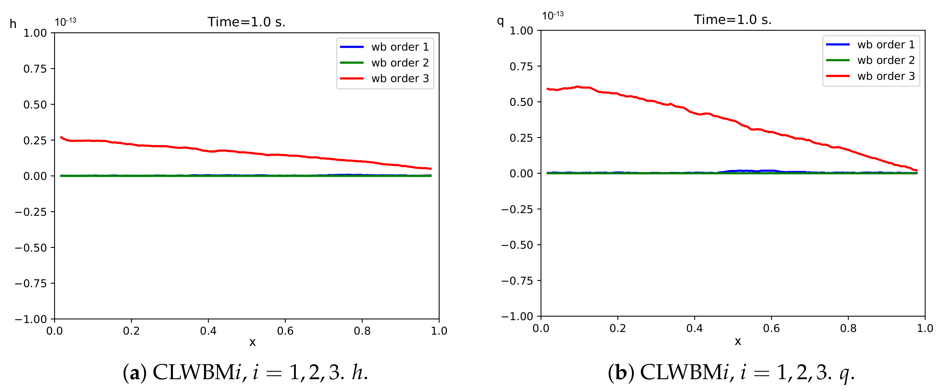
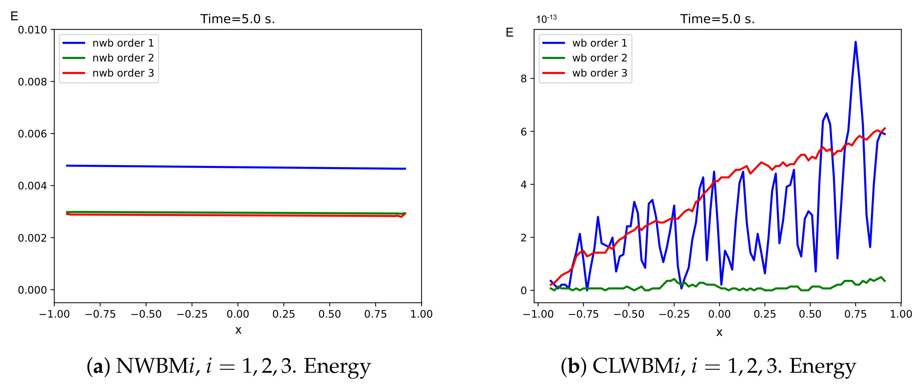
The numerical methods are integrated until the final time $t=5$, which is more than twice the travel time of a small perturbation of the steady state along the domain. $L^1$ errors between the initial and final cell-averages will be computed. According to Theorem 1, errors should be of the order of the machine precision (MP) if option (d) is considered to compute the initial condition for CLWBMi, $i=1,2,3$. Figure 1 (right) shows the errors corresponding to CLWBMi, $i=1,2,3$ for a 200-cell mesh. As expected, they are of the order of MP.

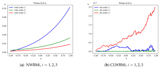
Figure 1. Test 1.1. Differences between the stationary and the numerical solutions at time $t=5$ s for a 200-cell mesh.

Notice that, in the other cases, if (a), (b), or (c) are used for CLWBMi, $i=1,2,3$, the errors decrease with $\mathsf{\Delta }x$ (see Table 1). Thus, if option (b) is chosen and a third order reconstruction operator is used, then the convergence rate is expected to be 4 as errors are generated by the use of the 2-stage collocation RK method for solving the local problems. If option (c) is used, the same convergence rate is expected, and the errors are due to the use of RK4 for computing the initial condition and the use of the 2-stage collocation RK method. Finally, in the case of option (a), the errors are due to the use of both numerical integration and the 2-stage collocation method in the solution of local problems: again, the errors are expected to be of order 4.

Table 1. Test 1.1. $L^1$ errors at $t=5$ and convergence rates for CLWBM3 when option (a), (b), (c), and (d) are chosen to compute the initial cell averages.

Cells	Option (a)		Option (b)		Option (c)		Option (d)
	Error	Order	Error	Order	Error	Order	Error	Order
5	1.96 × ${10}^{-4}$	-	1.82 × ${10}^{-4}$	-	1.46 × ${10}^{-4}$	-	4.88 × ${10}^{-16}$	-
10	1.21 × ${10}^{-5}$	4.015	1.12 × ${10}^{-5}$	4.016	8.81 × ${10}^{-6}$	4.054	7.44 × ${10}^{-16}$	-
20	7.56 × ${10}^{-7}$	4.003	7.01 × ${10}^{-7}$	4.003	5.42 × ${10}^{-7}$	4.023	3.00 × ${10}^{-16}$	-
40	4.72 × ${10}^{-8}$	4.001	4.38 × ${10}^{-8}$	4.001	3.36 × ${10}^{-8}$	4.011	7.94 × ${10}^{-15}$	-
80	2.95 × ${10}^{-9}$	4.000	2.74 × ${10}^{-9}$	4.000	2.09 × ${10}^{-9}$	4.006	9.00 × ${10}^{-15}$	-
160	1.84 × ${10}^{-10}$	4.000	1.71 × ${10}^{-10}$	4.000	1.30 × ${10}^{-10}$	4.003	1.23 × ${10}^{-14}$	-

Similar results are obtained for first and second-order methods: the order of convergence is two if option (a), (b), and (c) are used since the mid-point method is second-order accurate, and we consider the 1-stage collocation RK method.

Now, we compare the results obtained with NWBMi, WBMi, CWBMi, CLWBMi, $i=1,2,3$. The cell-averages are computed using option (b) for NWBMi and WBMi, option (c) for CWBMi, and option (d) for CLWBMi. $L^1$ errors with respect to the initial condition are computed.

Figure 1 shows the differences between the stationary and the numerical solutions obtained with NWBMi and CLWBMi, $i=1,2,3$. Similar results are obtanied for WBMi and CWBMi, $i=1,2,3$. Table 2 and Table 3 show the errors corresponding to NWBMi, WBMi, CWBMi, CLWBMi, $i=1,2,3$.

Table 2. Test 1.1. Differences in $L^1$-norm with respect to the stationary solution and convergence rates for NWBMi, $i=1,2,3$.

Cells	NWBM1: Error	Order	NWBM2: Error	Order	NWBM3: Error	Order
100	7.53 × ${10}^{-2}$	-	2.44 × ${10}^{-3}$	-	7.66 × ${10}^{-6}$	-
200	3.78 × ${10}^{-2}$	0.995	8.09 × ${10}^{-4}$	1.591	9.62 × ${10}^{-7}$	2.993
400	1.89 × ${10}^{-2}$	1.002	2.16 × ${10}^{-4}$	1.905	1.21 × ${10}^{-7}$	2.995
800	9.43 × ${10}^{-3}$	1.000	5.54 × ${10}^{-5}$	1.963	1.51 × ${10}^{-8}$	2.998

Table 3. Test 1.1. Differences in $L^1$-norm with respect to the stationary solution for WBMi, CWBMi, CLWBMi, $i=1,2,3$.

Cells	Order 1: Error			Order 2: Error			Order 3: Error
	WBM	CWBM	CLWBM	WBM	CWBM	CLWBM	WBM	CWBM	CLWBM
100	4.21 × ${10}^{-15}$	3.55 × ${10}^{-15}$	2.50 × ${10}^{-15}$	8.87 × ${10}^{-16}$	3.63 × ${10}^{-16}$	2.03 × ${10}^{-16}$	3.20 × ${10}^{-16}$	1.43 × ${10}^{-14}$	8.17 × ${10}^{-15}$
200	2.90 × ${10}^{-15}$	5.54 × ${10}^{-13}$	2.51 × ${10}^{-15}$	4.42 × ${10}^{-16}$	1.23 × ${10}^{-15}$	1.66 × ${10}^{-16}$	2.54 × ${10}^{-16}$	2.43 × ${10}^{-14}$	1.76 × ${10}^{-14}$
400	1.84 × ${10}^{-14}$	2.05 × ${10}^{-14}$	1.12 × ${10}^{-15}$	1.82 × ${10}^{-15}$	3.64 × ${10}^{-16}$	2.89 × ${10}^{-16}$	7.40 × ${10}^{-14}$	4.47 × ${10}^{-14}$	4.45 × ${10}^{-14}$
800	4.45 × ${10}^{-16}$	2.67 × ${10}^{-15}$	2.77 × ${10}^{-15}$	1.83 × ${10}^{-16}$	2.03 × ${10}^{-16}$	2.05 × ${10}^{-16}$	2.61 × ${10}^{-15}$	9.48 × ${10}^{-14}$	7.88 × ${10}^{-14}$

Notice that the errors for NWBM decrease with $\mathsf{\Delta }x$ at the expected rate. WBM preserve the exact solution up to MP, as well as CWBM and CLWBM, provided that the tolerance used in the Newton’s method for the former and Algorithm 5 for the latter is small enough. The computational costs are shown in Table 4. Nonetheless, since the goal of carrying out these experiments is to prove that the introduced well-balanced technique works, the implementation is not optimized. It can be seen that the well-balanced reconstruction given by Algorithm 2 increases the computational cost by a factor ranging from 1.5 to 7.5 (see Table 4). On the other hand, the use of Algorithm 3 increases the computational cost by a factor ranging from 1 to 1.8 if collocation RK method are used for solving the local problems and a factor ranging from 1.1 to 3.8 if control techniques with $N_p=1$ (see Reference [39]) are used. Therefore, the CLWBM schemes introduced in this work are more efficient than the CWBM schemes presented in Reference [39].

Table 4. Test 1.1. Computational times (milliseconds).

Cells	Order (i)	NWBMi	WBMi	CWBMi	CLWBMi
	1	20	30	70	30
100	2	30	60	140	110
	3	40	190	240	230
	1	20	60	230	100
200	2	40	190	330	280
	3	110	480	530	520
	1	50	180	520	220
400	2	100	530	1150	720
	3	350	1680	1980	1870
	1	140	570	2020	870
800	2	270	2040	3580	2820
	3	1080	5540	6600	5960

4.2. Problem 2: Burgers Equation with a Non-linear Source Term II

We now consider Burgers equation with another non-linear source term:

$$\left\{\begin{array}{c}{u}_t+{\left({\displaystyle \frac{u^2}{2}}\right)}_x=sin\left(u\right),x\in \mathbb{R},t>0,\hfill \\ u(x,0)=u_0\left(x\right).\hfill \end{array}\right.$$

(57)

The stationary solutions satisfy the ODE

$$u^{\prime }=\frac{sin\left(u\right)}{u}.$$

(58)

Note that no simple expression of the stationary solutions is known so (10) has to be computed numerically.

4.2.1. Test 2.1

We consider again the same computational domain, and the system is integrated up to $T=5$. The CFL parameter is imposed to be $0.9$. As initial condition, we consider the stationary solution that corresponds to the solution of the Cauchy problem (58) with

$$u(-1)=2,$$

that is approximated by the Gauss-Legendre collocation method. The left boundary condition is set to $u(-1,t)=2$, and open boundary conditions are considered upstream.

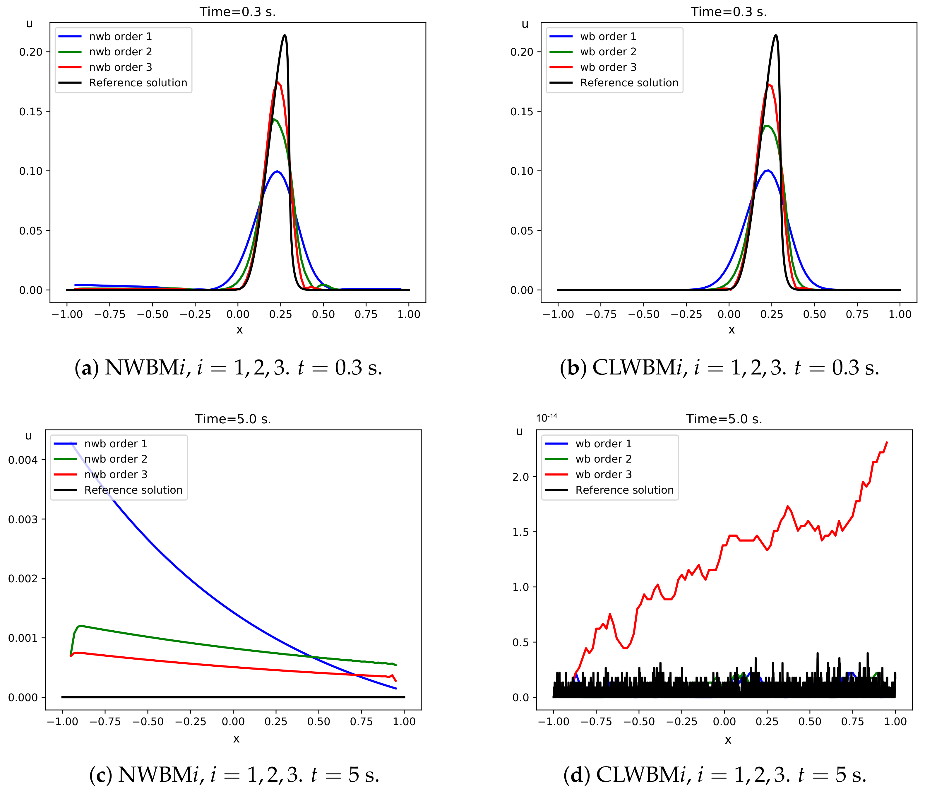
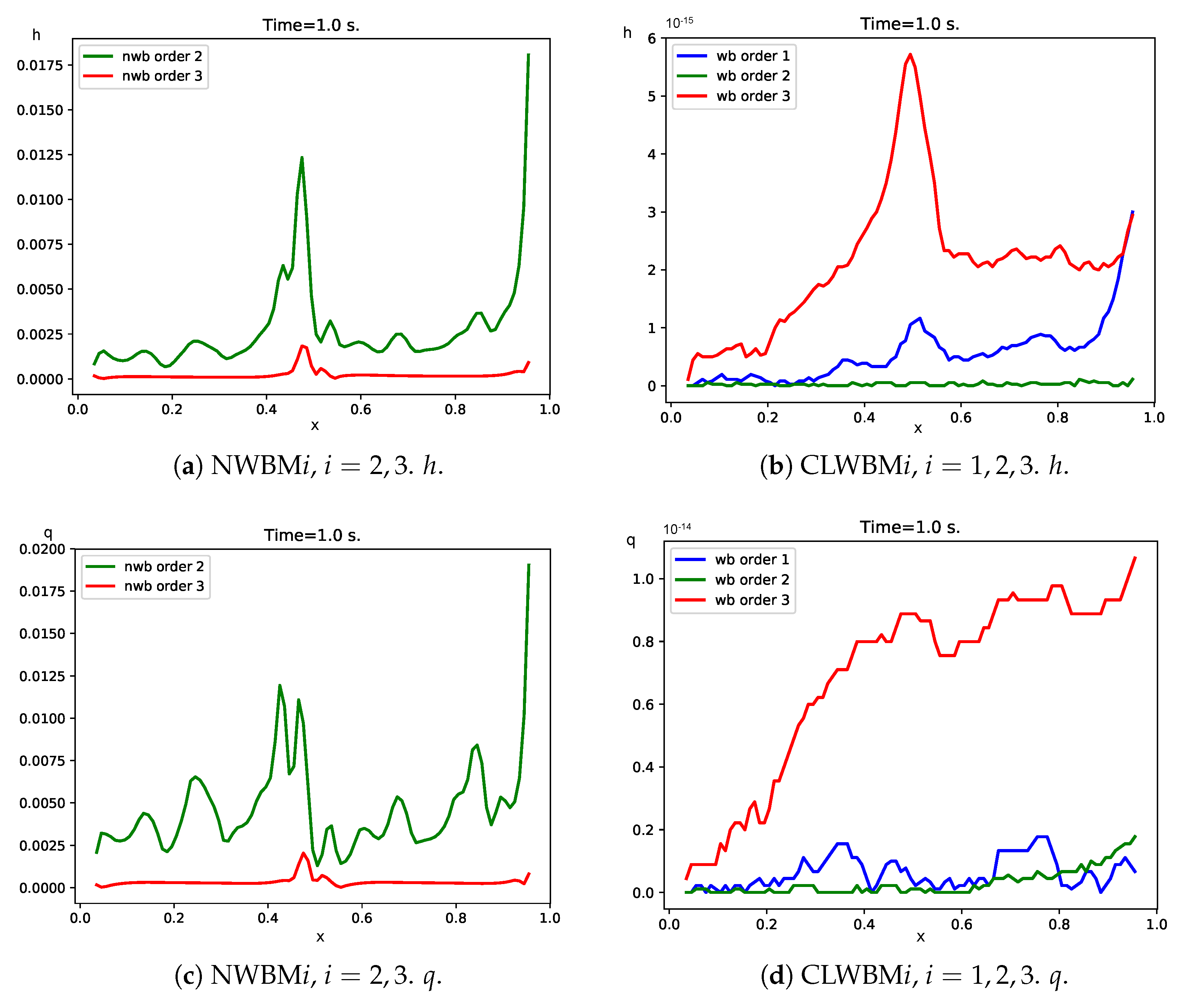
Figure 2 shows the differences between the stationary and the numerical solutions computed with NWBMi, $i=1,2,3$ (left) and CLWBMi, $i=1,2,3$ (right), (the figures corresponding to CWBMi, $i=1,2,3$ are similar).

Figure 2. Test 2.1. Differences between the stationary and the numerical solutions at $t=5$ s using a mesh with 100 cells.

The errors corresponding to NWBMi, CWBMi, and CLWBMi, $i=1,2,3$, respectively, are shown in Table 5 and Table 6. Computational costs are shown in Table 7. Note that the collocation strategy increases the computational cost from 7.3 to 14, whereas the method proposed in Reference [39] increases the computational cost by a factor ranging from 27 to 40. After the study of these two experiments, one can conclude that the results obtained with the collocation strategy introduced in this paper are better than the ones got by CWBMi, $i=1,2,3$ as described in Reference [39], considering that the errors are similar for both procedures, but the first strategy is much more efficient. Consequently, we will only consider the collocation strategy in the following experiments.

Table 5. Test 2.1. Differences in $L^1$-norm with respect to the stationary solution and convergence rates for NWBMi, $i=1,2,3$.

Cells	Error ($\mathit{i}=1$)	Order	Error ($\mathit{i}=2$)	Order	Error ($\mathit{i}=3$)	Order
100	2.72 × ${10}^{-3}$	-	1.43 × ${10}^{-4}$	-	2.53 × ${10}^{-5}$	-
200	1.34 × ${10}^{-3}$	1.021	2.43 × ${10}^{-6}$	5.879	1.74 × ${10}^{-8}$	10.503
400	6.58 × ${10}^{-4}$	1.026	8.19 × ${10}^{-7}$	1.569	1.14 × ${10}^{-10}$	7.250
800	3.24 × ${10}^{-4}$	1.022	2.34 × ${10}^{-7}$	1.806	1.41 × ${10}^{-11}$	3.016

Table 6. Test 2.1. Differences in $L^1$-norm with respect to the stationary solution for CWBMi, CLWBMi, $i=1,2,3$.

Cells	Order 1: Error		Order 2: Error		Order 3: Error
	CWBM	CLWBM	CWBM	CLWBM	CWBM	CLWBM
100	9.71 × ${10}^{-14}$	3.00 × ${10}^{-15}$	1.76 × ${10}^{-13}$	6.39 × ${10}^{-16}$	1.99 × ${10}^{-13}$	8.50 × ${10}^{-15}$
200	7.56 × ${10}^{-15}$	5.37 × ${10}^{-15}$	3.46 × ${10}^{-15}$	5.15 × ${10}^{-16}$	2.97 × ${10}^{-14}$	2.51 × ${10}^{-14}$
400	4.00 × ${10}^{-15}$	5.68 × ${10}^{-15}$	7.53 × ${10}^{-16}$	5.73 × ${10}^{-16}$	3.31 × ${10}^{-14}$	4.85 × ${10}^{-14}$
800	5.97 × ${10}^{-15}$	4.63 × ${10}^{-15}$	8.54 × ${10}^{-16}$	5.31 × ${10}^{-16}$	6.63 × ${10}^{-14}$	9.61 × ${10}^{-14}$

Table 7. Test 2.1. Computational cost (milliseconds). $t=5$ s.

Cells	Order(i)	NWBMi	CWBMi	CLWBMi
	1	10	340	130
100	2	20	690	280
	3	40	1390	490
	1	30	1280	230
200	2	60	2350	440
	3	180	5190	1230

4.2.2. Test 2.2

Now, we consider the evolution of a small perturbation of the previous stationary solution. Thus, the initial solution is set to

$$u_0\left(x\right)=u^{*}\left(x\right)+0.3e^{-200{(x+0.5)}^2},$$

where $u^{*}\left(x\right)$ is the previous stationary solution.

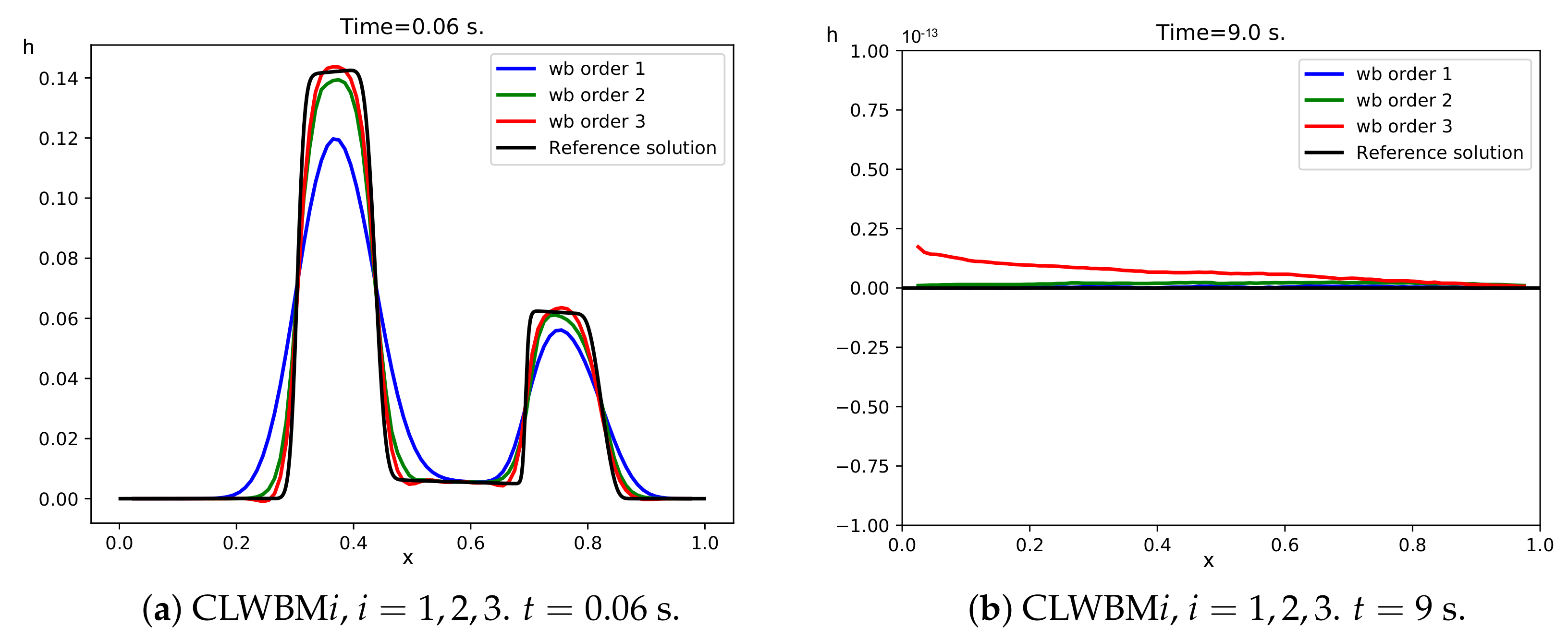
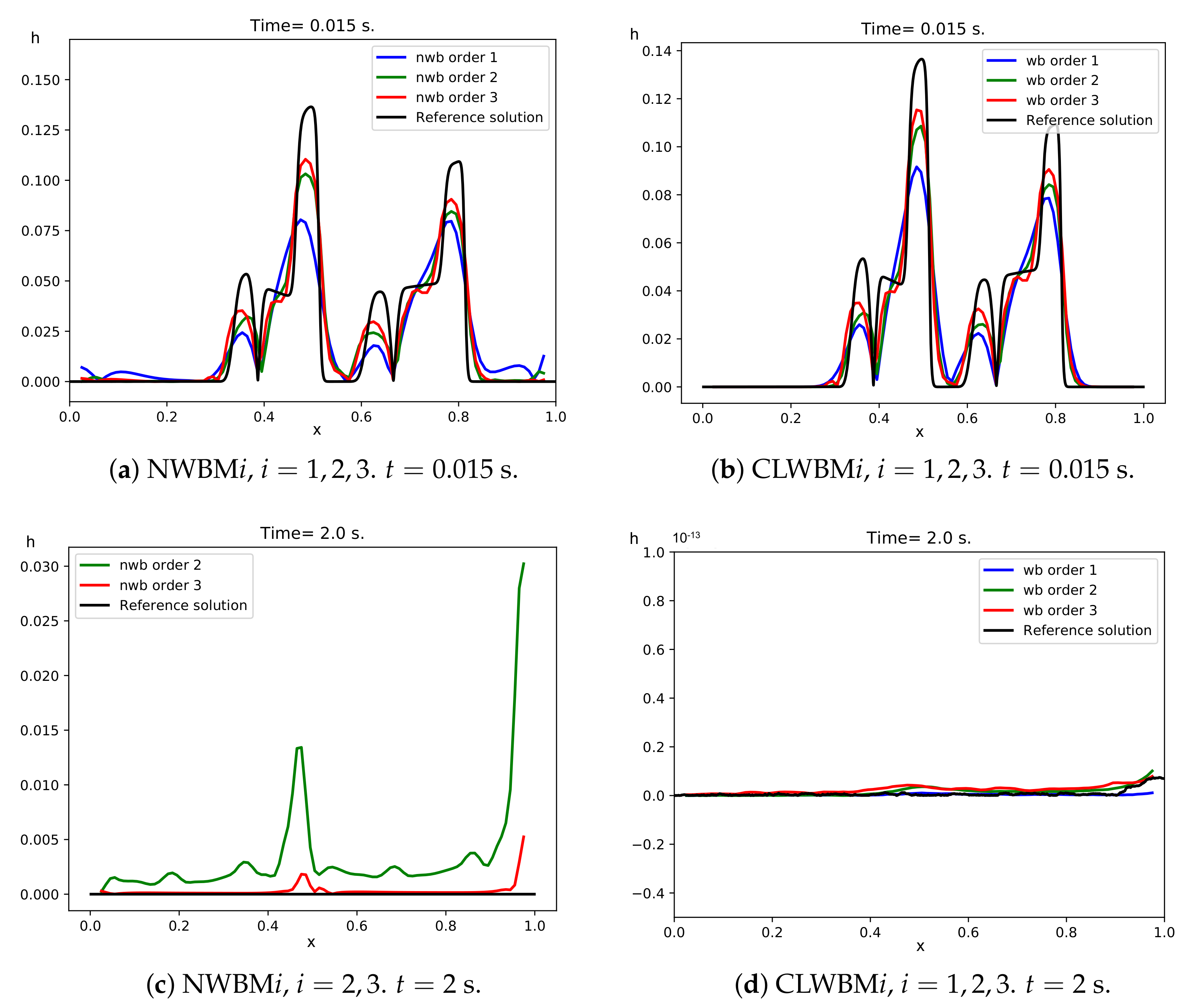
Figure 3 shows the difference between the stationary and the numerical solutions computed with NWBMi, $i=1,2,3$ and CLWBMi, $i=1,2,3$ at times $t=0.3,5$ (the results are similar for CWBMi, $i=1,2,3$). In black, we show a reference solution computed on a fine mesh with 12,800 cells using a first order well-balanced method.

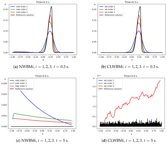
Figure 3. Test 2.2. Reference and numerical solutions: differences with the stationary solution at times $t=0.3,5$ s for a 100-cell mesh.

Observe that, as expected, the well-balanced methods are able to recover the stationary solution after the perturbation left the domain, while non-well balanced methods introduce an error that remains in the domain. This could be also observed in Table 8, where the errors with respect to the stationary solution at time $t=5$ s are shown for the 100-cell mesh.

Table 8. Test 2.2. Differences in $L^1$-norm with respect to the stationary solution for NWBMi, CWBMi, and CLWBMi ($i=1,2,3$) at time $t=5$ s.

Method	Error ($\mathit{i}=1$)	Error ($\mathit{i}=2$)	Error ($\mathit{i}=3$)
NWBMi	2.43 × ${10}^{-3}$	1.71 × ${10}^{-3}$	1.05 × ${10}^{-3}$
CWBMi	1.09 × ${10}^{-13}$	4.47 × ${10}^{-15}$	3.34 × ${10}^{-14}$
CLWBMi	2.52 × ${10}^{-15}$	1.19 × ${10}^{-15}$	1.24 × ${10}^{-14}$

4.3. Problem 3: Shallow Water Equations

Let us consider now the 1D shallow water system which corresponds to the choices $N=2$, with

$$U=\left(\begin{array}{c}h\\ q\end{array}\right),f\left(U\right)=\left(\begin{array}{c}q\\ {\displaystyle \frac{q^2}{h}+\frac{g}{2}{h}^2}\end{array}\right),S\left(U\right)=\left(\begin{array}{c}0\\ gh\end{array}\right),$$

where x corresponds to to the axis of the channel, and t is the time. The unknown $h(x,t)$ and $q(x,t)$ are the thickness and discharge, respectively; the function $H\left(x\right)$ is the depth function, and g is the gravity; $u=q/h$ is the depth-averaged velocity, and $c=\sqrt{gh}$.

The eigenvalues of the system are ${\lambda }^{\pm }=u\pm c$, and the Froude number defined by

$${\displaystyle Fr\left(U\right)=\frac{\left|u\right|}{c},}$$

(59)

characterizes the flow regime: subcritical ($Fr>1$), critical ($Fr=1$), or supercritical ($Fr>1$).

The stationary solutions $U^{*}$ satisfy the ODE system:

$$\left\{\begin{array}{c}{q}_x=0,\hfill \\ {\left({\displaystyle \frac{q^2}{h}+\frac{1}{2}g{h}^2}\right)}_x=gh{H}_x,\hfill \end{array}\right.$$

(60)

which can be written as follows:

$$\left\{\begin{array}{c}\left(-u^2+gh\right)h_x=gh{H}_x,\hfill \\ q_x=0.\hfill \end{array}\right.$$

(61)

The stationary solutions are given in implicit form by:

$$q=C_1,\frac{q^2}{2h^2}+gh-gH=C_2,C_1,C_2\in \mathbb{R}.$$

(62)

In Reference [38], a family of high-order well-balanced numerical methods was presented, based in the Algorithm 2, in which local problems were solved on the basis of this implicit form. Here, Algorithm 3 with collocation RK methods to solve the local problems is used.

The numerical treatment of resonant situations discussed in Section 3.6 will be illustrated here in the particular case of the shallow water system. It can be easily checked that system (50), which, in our case, becomes

$$\left[\begin{array}{cc}0& 1\\ -u^2+gh& 2u\end{array}\right]\left[\begin{array}{c}{K}_1\\ K_2\end{array}\right]=\left[\begin{array}{c}0\\ gh{H}_x\left(x\right)\end{array}\right],$$

(63)

when $U^{*}$ is a critical state, i.e., when $u^2=gh$, reduces to:

$$\left[\begin{array}{cc}0& 1\\ 0& 2u\end{array}\right]\left[\begin{array}{c}{K}_1\\ K_2\end{array}\right]=\left[\begin{array}{c}0\\ gh{H}_x\left(x\right)\end{array}\right].$$

(64)

Therefore, the system has solutions only if $H_x\left(x\right)=0$: in this case, the solutions are

$$K=\alpha {[1,0]}^T,\alpha \in \mathbb{R}.$$

In fact, it can be shown (see Reference [38], for instance) that a smooth stationary solution can only reach a critical state at a minimum point $x^c$ of the depth function H. Differentiating the second relation of (62) with respect to x, and using the relation $H_x\left(x_c\right)=0$, one obtains, at $x=x_c$,

$$\frac{q{q}_x}{h^2}+h_x\left(g-\frac{q^2}{h^3}\right)=0,$$

which, assuming $h_x\left(x_c\right)\ne 0$, implies

$${\displaystyle h^c\left(q\right)=\frac{q^{2/3}}{g^{1/3}}.}$$

(65)

With this information in mind, let us compute the limit

$$\underset{x\to x^c}{lim}\frac{gh{H}_x}{-u^2+gh},$$

to determine the value of $h_x$ at $x^c$. This is a $0/0$ indeterminate limit, and L’Hôpital’s rule can be applied. To do this, first, the limit is rewritten as follows:

$$\underset{x\to x^c}{lim}\frac{g{H}_x}{{\displaystyle g-\frac{q^2}{h^3}}}.$$

(66)

Some easy computation leads to

$$h_x\left(x^c\right)=\frac{h^c{\left(q\right)}^4}{3h_x\left(x^c\right)q^2}g{H}_{xx}\left(x^c\right);$$

(67)

therefore:

$$h_x\left(x^c\right)=\pm \frac{h^c{\left(q\right)}^2}{\sqrt{3}q}{g}^{1/2}\sqrt{H_{xx}\left(x^c\right)}=\pm \sqrt{\frac{h^c\left(q\right)H_{xx}\left(x^c\right)}{3}}=\pm \sqrt{\frac{q^{2/3}{H}_{xx}\left(x^c\right)}{3g^{1/3}}}.$$

(68)

The above expression shows that, if $q\ne 0$ and $H_{xx}\left(x_c\right)\ne 0$, it is $h_x\left(x_c\right)\ne 0$, thus justifying the assumption used before. Then, the chosen solution of (50) will be

$$K={\left[\pm \sqrt{\frac{q^{2/3}{H}_{xx}\left(x^c\right)}{3g^{1/3}}},0\right]}^T.$$

More precisely, when applying Algorithm 5 or Algorithm 4, a threshold $ϵ>0$ is selected to detect critical states. If a system (50) has to be solved in which

$$\left|Fr\right(U^{*})-1|<ϵ,$$

at a point $\overline{x}$, then

• If $\overline{x}$ is not close to a minimum point of H, it is assumed that is not possible to find a smooth stationary solution that solves the problem and the algorithm is stopped.
• Otherwise, the selected solution of (50) is

  -

  $K={\left[{\displaystyle \sqrt{\frac{q^{2/3}{H}_{xx}\left(\overline{x}\right)}{3g^{1/3}}},0}\right]}^T$, if h is increasing close to $\overline{x}$,

  -

  $K={\left[{\displaystyle -\sqrt{\frac{q^{2/3}{H}_{xx}\left(\overline{x}\right)}{3g^{1/3}}},0}\right]}^T$, if h is decreasing close to $\overline{x}$,

  and the algorithm goes on.

4.3.1. Test 3.1: Transcritical Smooth Stationary Solution

The objective with this test is to check the correct behavior of the numerical methods of this work in presence of critical states. Following Reference [38], we consider here a smooth transcrital stationay solution for the 1D shallow water system on the interval $[0,3]$. The integration time is $T=1$, and the bathymetry is given by

$$H\left(x\right)=\left\{\begin{array}{ccc}-0.25(1+cos(5\pi (x+0.5)\left)\right)\hfill & \mathrm{if}& 1.3\le x\le 1.7,\\ \\ 0\hfill & & \mathrm{otherwise}.\end{array}\right.$$

(69)

The initial condition corresponds to the solution of the Cauchy problem (61) with initial condition $h\left(0\right)=1.67750727$ and $q\left(0\right)=2.5$. It can be checked that it has a critical state at $x^c=1.5$. The shallow water system is integrated up to time $T=1$, setting q downstream, and the water height upstream. The difference between the stationary and the numerical solutions computed with NWBMi, $i=1,2,3$ and CLWBMi, $i=1,2,3$ are shown in Figure 4. $L^1$ Errors are shown in Table 9 and Table 10. Notice that Reference [38] obtained similar results. The computational costs are shown in Table 11.

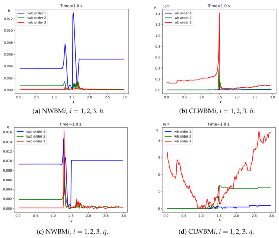
Figure 4. Test 3.1. Reference and numerical solutions: differences with the stationary solution at time $t=1$ s for the 200-cell mesh.

Table 9. Test 3.1. Differences in $L^1$-norm with respect to the stationary solution and convergence rates for NWBMi, $i=1,2,3$.

Cells	Error ($\mathit{i}=1$)	Order	Error ($\mathit{i}=2$)	Order	Error ($\mathit{i}=3$)	Order
	$\mathit{h}$		$\mathit{h}$		$\mathit{h}$
100	4.99 × ${10}^{-2}$	-	7.63 × ${10}^{-3}$	-	5.99 × ${10}^{-3}$	-
200	1.31 × ${10}^{-2}$	1.923	1.27 × ${10}^{-3}$	2.583	8.86 × ${10}^{-4}$	2.757
400	3.87 × ${10}^{-3}$	1.766	1.84 × ${10}^{-4}$	2.790	6.20 × ${10}^{-5}$	3.838
800	1.56 × ${10}^{-3}$	1.314	5.31 × ${10}^{-5}$	1.794	6.88 × ${10}^{-6}$	3.172
Cells	Error ($\mathit{i}=\mathbf{1}$)	Order	Error ($\mathit{i}=\mathbf{2}$)	Order	Error ($\mathit{i}=\mathbf{3}$)	Order
	$\mathit{q}$		$\mathit{q}$		$\mathit{q}$
100	1.28 × ${10}^{-1}$	-	1.89 × ${10}^{-2}$	-	1.72 × ${10}^{-2}$	-
200	2.81 × ${10}^{-2}$	2.188	3.18 × ${10}^{-3}$	2.575	2.35 × ${10}^{-3}$	2.866
400	9.29 × ${10}^{-3}$	1.161	4.81 × ${10}^{-4}$	2.724	2.09 × ${10}^{-4}$	3.489
800	4.09 × ${10}^{-3}$	1.168	1.37 × ${10}^{-4}$	1.812	2.29 × ${10}^{-5}$	3.190

Table 10. Test 3.1. Differences in $L^1$-norm with respect to the stationary solution for CLWBMi, $i=1,2,3$.

Cells	Error (i = 1)		Error (i = 2)		Error (i = 3)
	$\mathit{h}$	$\mathit{q}$	$\mathit{h}$	$\mathit{q}$	$\mathit{h}$	$\mathit{q}$
100	1.46 × ${10}^{-15}$	2.13 × ${10}^{-15}$	2.80 × ${10}^{-16}$	1.44 × ${10}^{-15}$	2.88 × ${10}^{-16}$	3.63 × ${10}^{-15}$
200	4.95 × ${10}^{-16}$	3.00 × ${10}^{-16}$	3.03 × ${10}^{-15}$	1.44 × ${10}^{-14}$	3.94 × ${10}^{-14}$	5.53 × ${10}^{-14}$
400	2.94 × ${10}^{-16}$	1.74 × ${10}^{-15}$	4.75 × ${10}^{-16}$	1.20 × ${10}^{-15}$	8.89 × ${10}^{-14}$	1.45 × ${10}^{-13}$
800	1.50 × ${10}^{-15}$	6.92 × ${10}^{-15}$	3.25 × ${10}^{-16}$	1.21 × ${10}^{-15}$	1.04 × ${10}^{-13}$	1.55 × ${10}^{-13}$

Table 11. Test 3.1. Computational cost (milliseconds). $t=1$ s.

Cells	Order (i)	NWBMi	CLWBMi
	1	20	30
100	2	30	130
	3	70	320
	1	30	60
200	2	80	370
	3	200	1100

4.3.2. Test 3.2: Perturbation of a Smooth Transcritical Stationary Solution

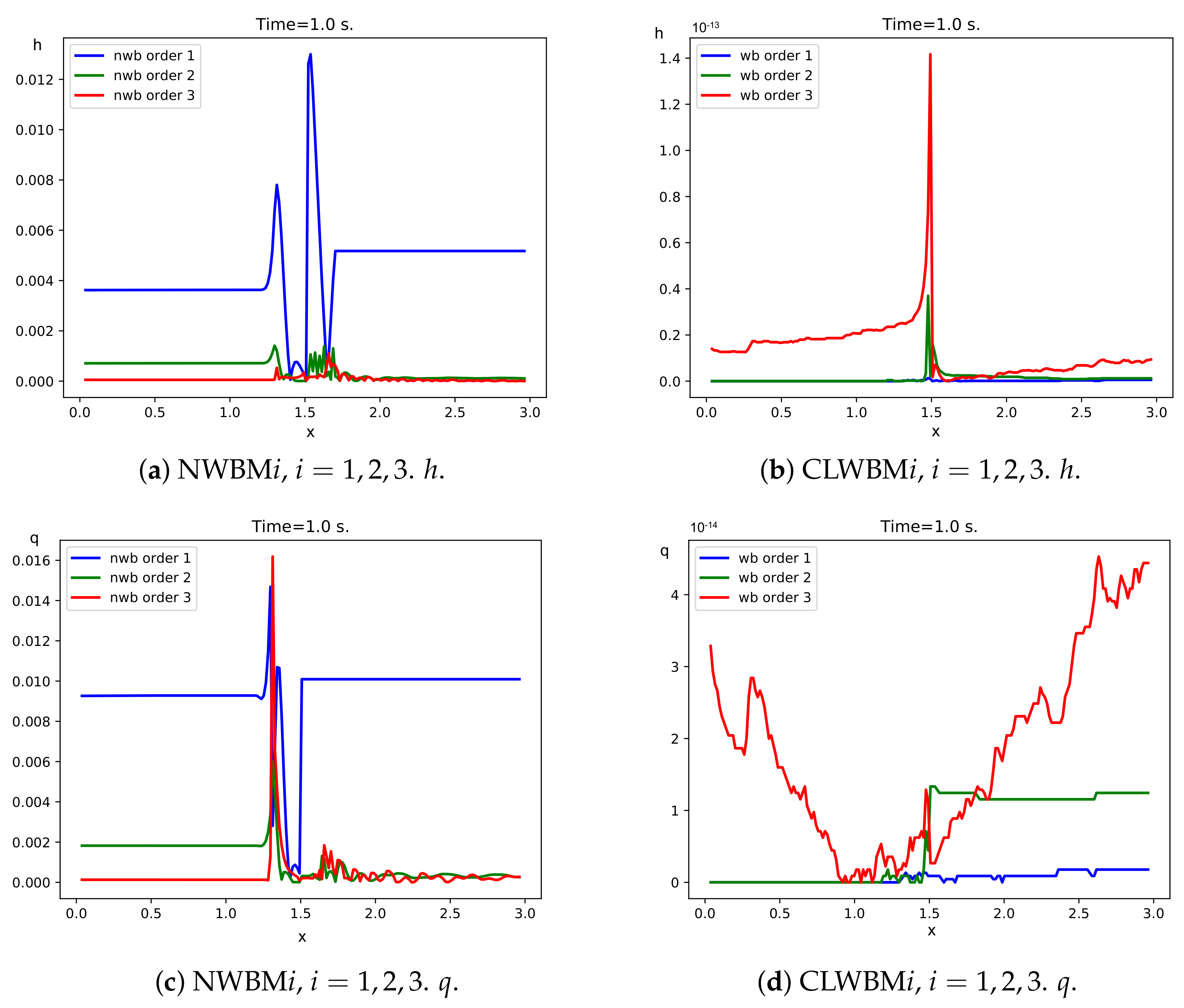
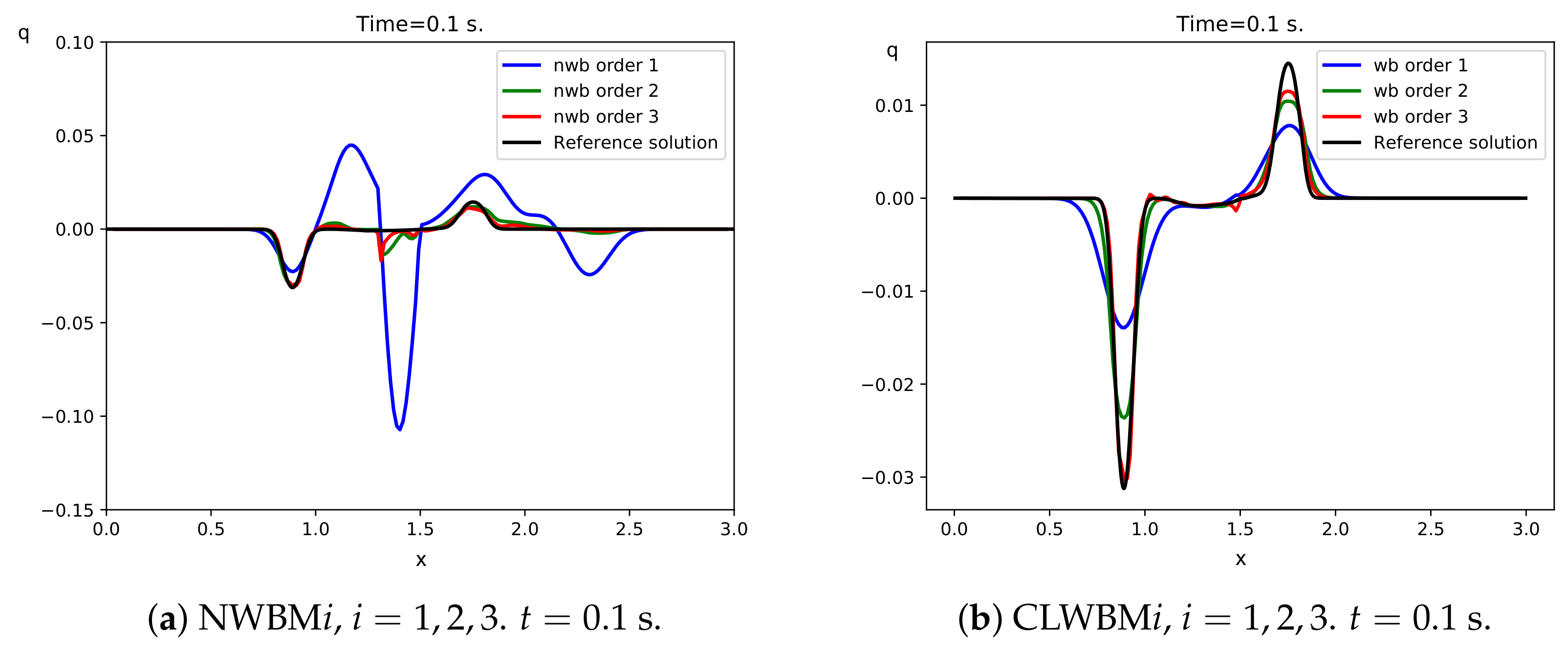
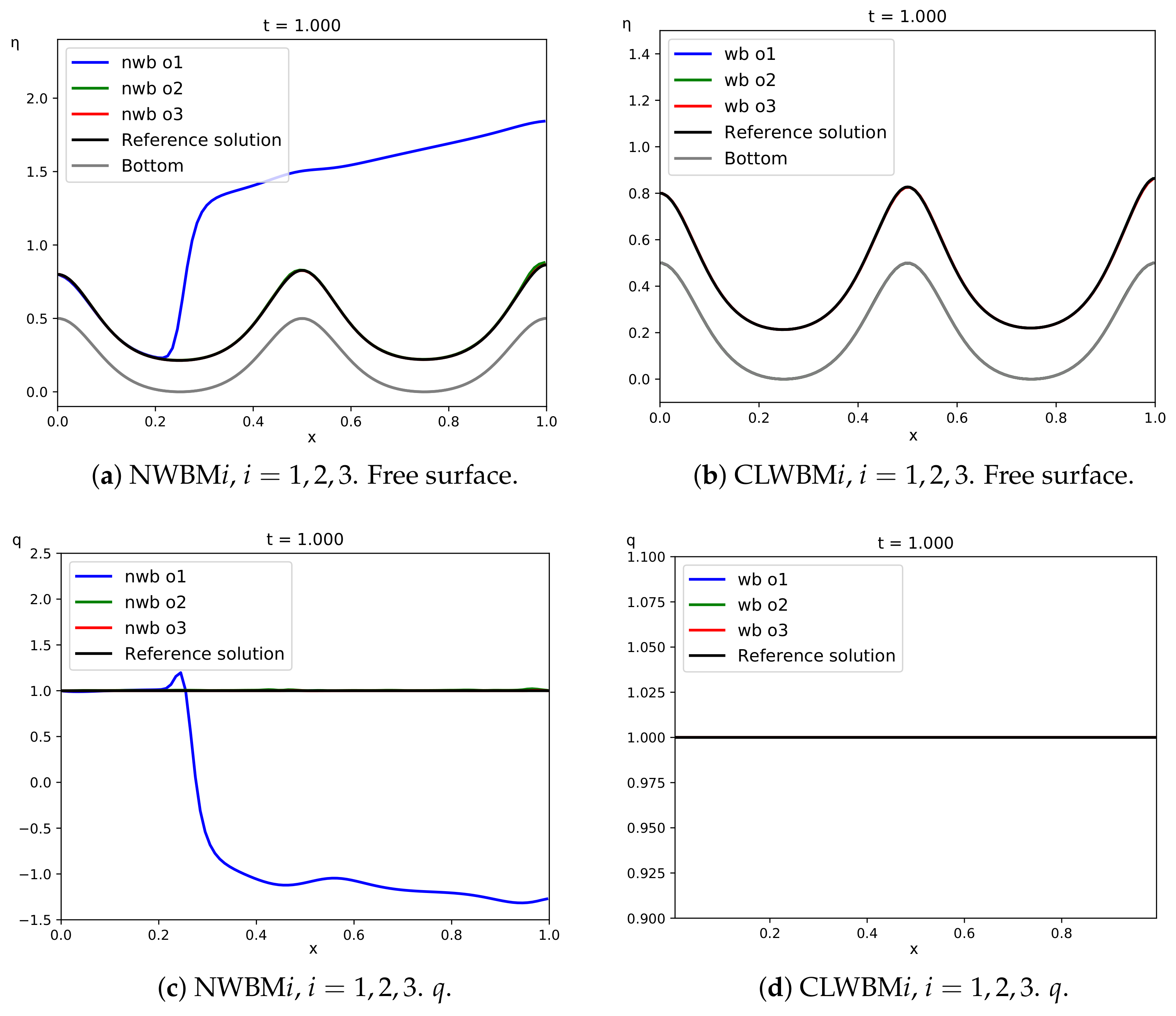
In this test, we consider the evolution of a small perturbation of the previous transcritical stationary solution. More precisely, a small perturbation of the water thickness of amplitude $\mathsf{\Delta }h=0.02$ is set at the interval $[1.1,1.2]$, that is in the subcritical region. Therefore, this perturbation splits in two wawes, one moving downstream and the other upstream, as shown in Figure 5 and Figure 6 at time $t=0.1$ s. Figure 5 and Figure 6 show the difference between the stationary and the numerical solutions computed with NWBMi, $i=1,2,3$ and CLWBMi, $i=1,2,3$ at times $t=0.1,5$ s. A reference solution is also computed using a first order well-balanced method with fine mesh (2000 cells).

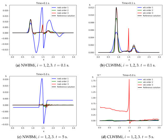
Figure 5. Test 3.2. Reference and numerical solutions: differences with the stationary solution at times $t=0.1,5$ s for h with a 200-cell mesh.

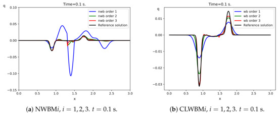
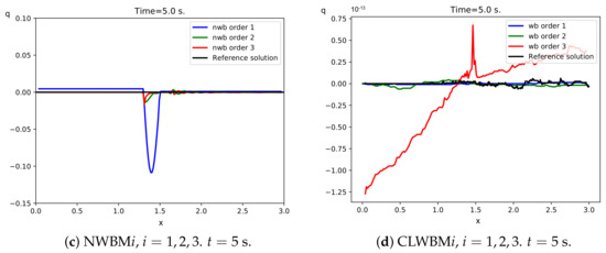
Figure 6. Test 3.2. Reference and numerical solutions: differences with the stationary solution at times $t=0.1,5$ s for q for a 200-cell mesh.

Observe that, as in the previous examples, only the well-balanced methods are able to preserve the stationary solution. The non-well-balanced method generates strong perturbations that are bigger than the initial perturbation. Differences between the stationary and the numerical solutions in $L^1$-norm at time $t=5$ s for a 200-cell mesh are shown in Table 12. Finally, let us point out that the third order well-balanced method presents a small spurious oscillation in the location of the critical point, that disappears with time. This is not the case for the first and second order well-balanced methods.

Table 12. Test 3.2. Differences in $L^1$-norm for NWBMi and CLWBMi ($i=1,2,3$) with respect to the stationary solution using a 200-cell mesh at time $t=5$ s.

Method	Error ($\mathit{i}=1$)		Error ($\mathit{i}=2$)		Error ($\mathit{i}=3$)
	$\mathit{h}$	$\mathit{q}$	$\mathit{h}$	$\mathit{q}$	$\mathit{h}$	$\mathit{q}$
NWBMi	1.01 × ${10}^{-2}$	2.13 × ${10}^{-2}$	4.83 × ${10}^{-4}$	2.00 × ${10}^{-3}$	2.70 × ${10}^{-4}$	1.30 × ${10}^{-3}$
CLWBMi	5.11 × ${10}^{-14}$	4.32 × ${10}^{-16}$	1.95 × ${10}^{-14}$	6.47 × ${10}^{-15}$	7.89 × ${10}^{-14}$	1.38 × ${10}^{-13}$

4.3.3. Test 3.3: Perturbation of a Smooth Subcritical Stationary Solution

Let us consider evolution of a small perturbation of a smooth subcritical stationary solution. The initial condition $U_0\left(x\right)={(h_0\left(x\right),q_0\left(x\right))}^T$ is given by:

$$h_0\left(x\right)=\left\{\begin{array}{cc}{h}^{*}\left(x\right)+0.02,\hfill & \mathrm{if} 0.7\le x\le 1.0,\hfill \\ h^{*}\left(x\right),\hfill & \mathrm{otherwise},\hfill \end{array}\right.$$

$$q_0\left(x\right)=q^{*}\left(x\right),$$

where $U^{*}\left(x\right)={(h^{*}\left(x\right),q^{*}\left(x\right))}^T$ is the solution of the Cauchy problem

$$\left\{\begin{array}{c}{q}_x=0,\hfill \\ \left(-u^2+gh\right)h_x=gh{H}_x,\hfill \\ h\left(0\right)=2,q\left(0\right)=3.5.\hfill \end{array}\right.$$

(70)

The depth function is given again by (69).

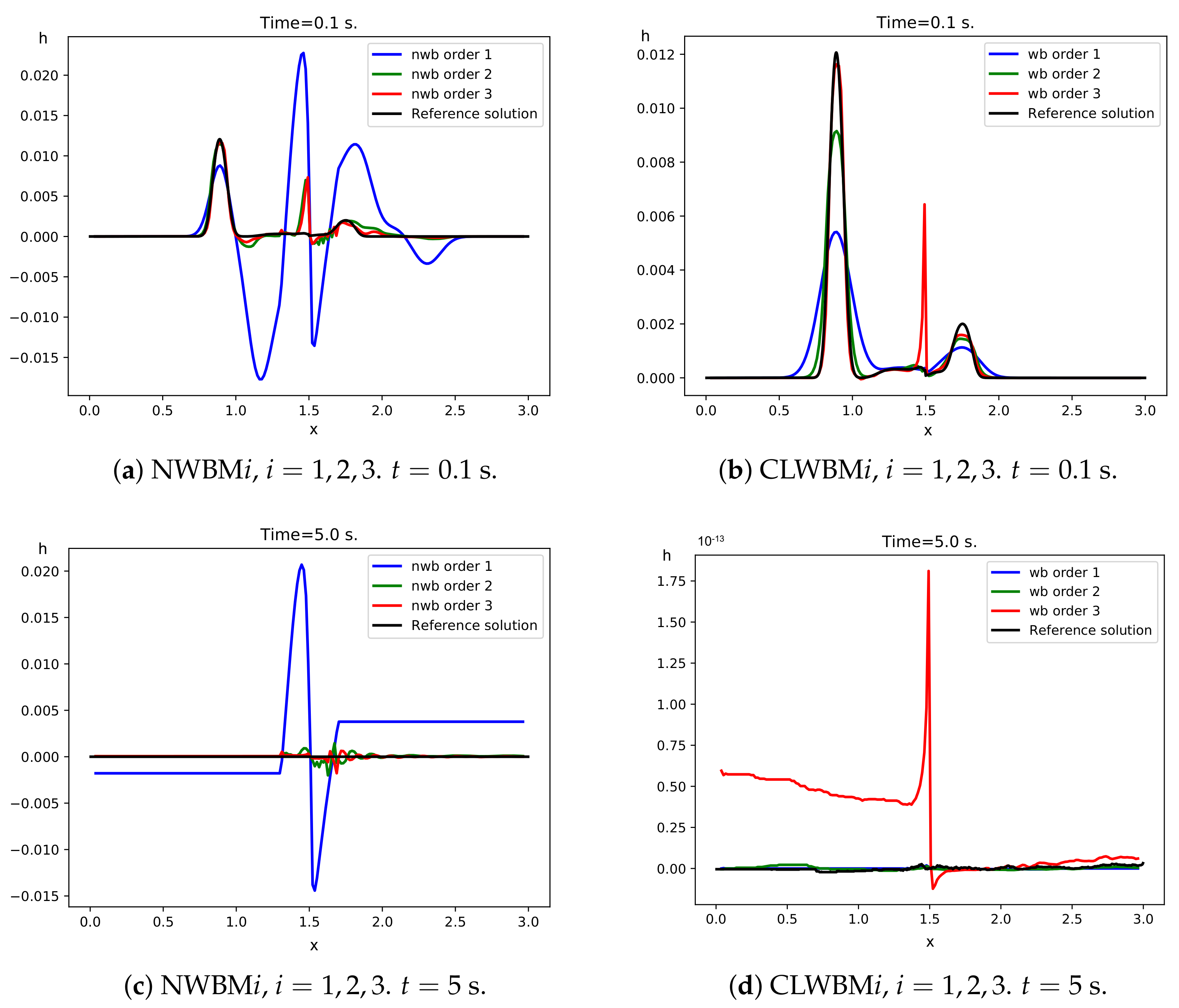
Figure 7 shows the differences between the stationary solution and the numerical solutions obtained with NWBMi, $i=1,2,3$ and CLWBMi, $i=1,2,3$ at times $t=0.1,5$ for h (the graphs are similar for q). A reference solution has been computed with a first order well-balanced scheme on a fine mesh (3200 cells).

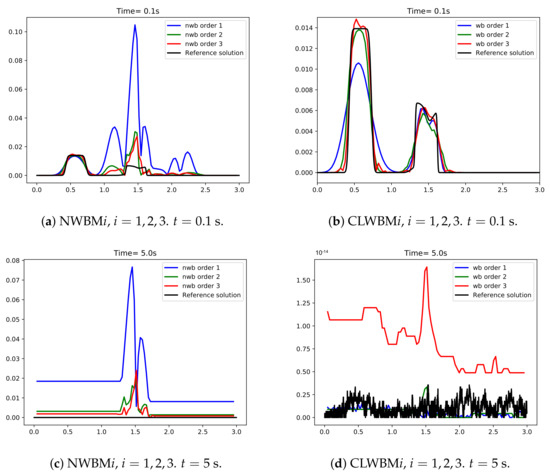
Figure 7. Test 3.3. Reference and numerical solutions: differences with the stationary solution at times $t=0.1$ s and $t=5$ s for h for a 100-cell mesh.

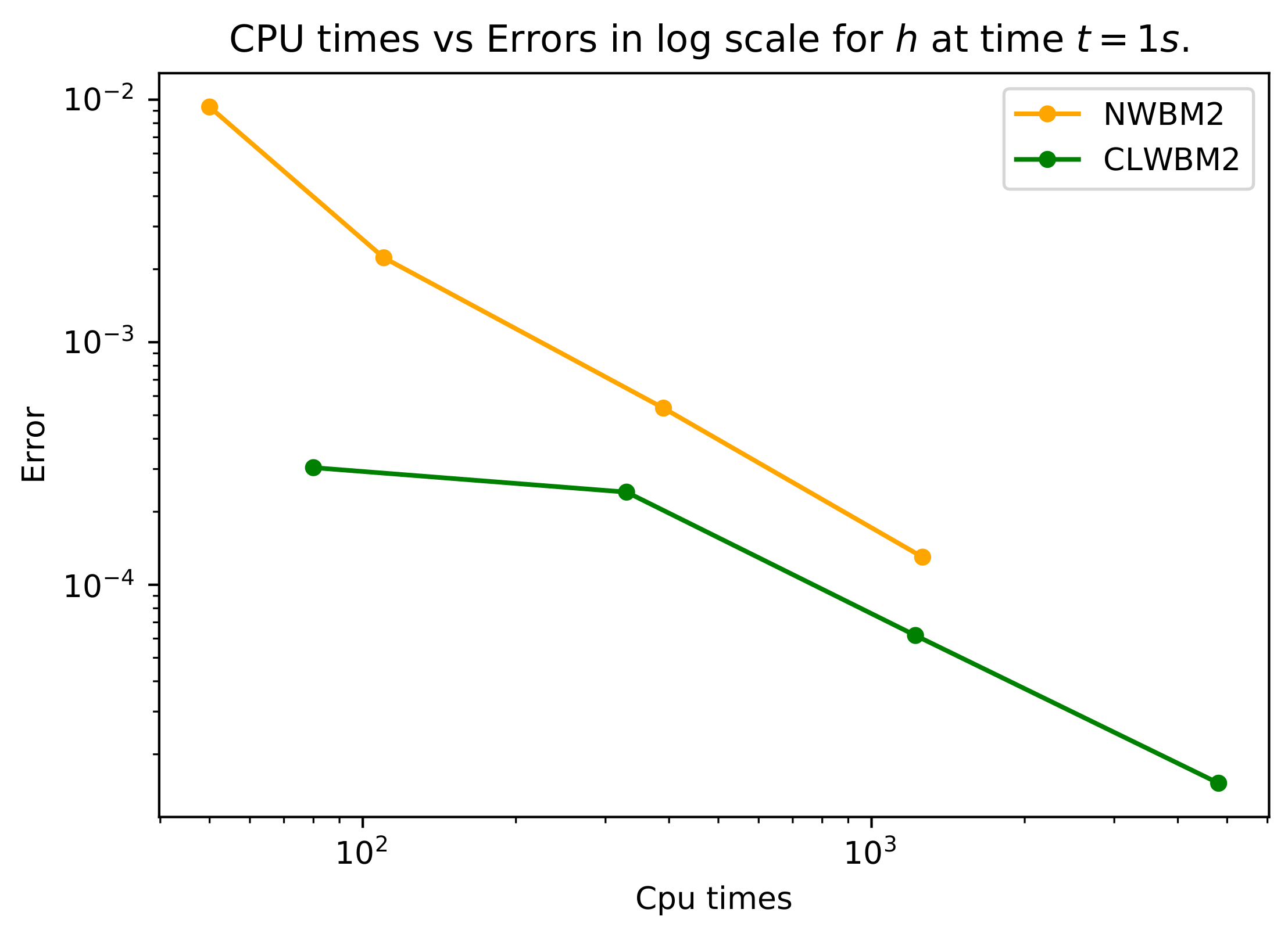
Notice that, since the perturbation amplitude is small enough, the well-balanced methods perform much better than the non-well-balanced methods, that generates spurious waves of amplitudes bigger than the original perturbation. In Table 13, the differences with respect to the stationary solution at time $t=5$ s are shown for the 100-cell mesh. In order to check the efficiency of the methods, Figure 8 shows the errors in $L^1$-norm with respect to the reference solution versus the CPU times in milliseconds for the NWBM2 and CLWBM2 at time $t=1$ s, when the perturbation is still in the domain. Similar results have been obtained for the first and third order methods. Notice that the CLWBM are computationally more efficient. See, for instance, that, in order to obtain an error of approximately 2 × ${10}^{-4}$, the computational cost for the NWBM2 is increased by a factor of about 2.2 with respect to the CLWBM2.

Table 13. Test 3.3. Differences in $L^1$-norm for NWBMi and CLWBMi ($i=1,2,3$) with respect to the stationary solution for the 100-cell mesh at time $t=5$ s.

Method	Error ($\mathit{i}=1$)		Error ($\mathit{i}=2$)		Error ($\mathit{i}=3$)
	$\mathit{h}$	$\mathit{q}$	$\mathit{h}$	$\mathit{q}$	$\mathit{h}$	$\mathit{q}$
NWBMi	5.08 × ${10}^{-2}$	1.94 × ${10}^{-1}$	9.33 × ${10}^{-3}$	3.51 × ${10}^{-2}$	6.02 × ${10}^{-3}$	2.12 × ${10}^{-2}$
CLWBMi	1.81 × ${10}^{-15}$	5.54 × ${10}^{-15}$	1.95 × ${10}^{-15}$	4.45 × ${10}^{-15}$	2.46 × ${10}^{-14}$	5.20 × ${10}^{-14}$

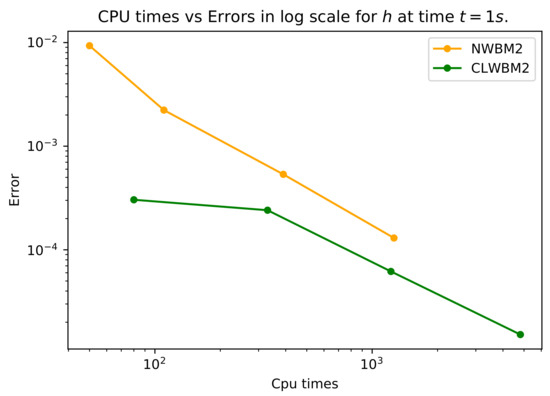
Figure 8. Test 3.3. Errors in $L^1$-norm with respect to the reference solution versus CPU times in milliseconds for the NWBM2 and CLWBM2 at time $t=1$ s.

4.4. Problem 4: Shallow Water Equations with Manning Friction

Let us consider the shallow water equations with Manning friction:

$$\left\{\begin{array}{c}{h}_t+q_x=0,\hfill \\ {\displaystyle q_t+{\left({\displaystyle \frac{q^2}{h}+\frac{1}{2}g{h}^2}\right)}_x=gh{H}_x-\frac{kq\left|q\right|}{h^{\eta }}.}\hfill \end{array}\right.$$

(71)

In the previous, k is the Manning friction coefficient, and $\eta$ is set to $\frac{7}{3}$.

The stationary solutions satisfy the ODE system

$$\left\{\begin{array}{c}{\displaystyle \left(-u^2+gh\right)h_x=gh{H}_x-\frac{kq\left|q\right|}{h^{\eta }},}\hfill \\ q_x=0.\hfill \end{array}\right.$$

(72)

In what follows, we consider some experiments taken from Reference [47].

4.4.1. Test 4.1

Let us consider first a moving equilibria test with constant bathymetry. Therefore, the smooth stationary solutions satisfy

$$\left\{\begin{array}{c}{\displaystyle \left(-q^2/h^2+gh\right)h_x=-\frac{kq\left|q\right|}{h^{\eta }},}\hfill \\ q_x=0.\hfill \end{array}\right.$$

(73)

As in Reference [47], we consider the interval the space interval $[0,1]$, discretized with 200 cells. Now, we consider a subcritical steady state with $q\left(0\right)=-1$ and $h\left(0\right)$ a positive root of the non-linear function $\xi \left(h\right)$, obtained by integrating (73), given by

$${\displaystyle \xi \left(h\right)=-\frac{q_0^2}{\eta -1}\left(h^{\eta -1}-h_0^{\eta -1}\right)+\frac{g}{\eta +2}\left(h^{\eta +2}-h_0^{\eta +2}\right)+k{q}_0\left|q_0\right|(x-x_0),}$$

(74)

where $x_0=-\mathsf{\Delta }x$, $x=0$, $q_0=q\left(0\right)$ and $h_0=h^c,$ with $h^c$ defined by

$$h^c={\left({\displaystyle \frac{q_0^2}{g}}\right)}^{\frac{1}{3}}.$$

In this experiment, $k=1$, which enforces the stiff character of the friction term. As boundary conditions, q is set downstream and h upstream, and the system is integrated up to $t=1$. Due to the stiff character of the friction term, the explicit non-well-balanced methods turn out to be unstable for small values of h and/or big values of k, unless a very small time step is used. If an implicit discretization of the stiff source term is considered, NWBMi, $i=1,2,3$ methods do not explode, yet there is not convergence to any stationary solution. The stability restriction is much less severe for the well-balanced schemes. For these reasons, only the numerical solutions obtained with well-balanced schemes are shown.

Figure 9 shows the discrepancies between the stationary and the numerical solutions at $t=1$ s with CLWBMi, $i=1,2,3$; Table 14 shows the $L^1$ errors for a mesh with 200 cells.

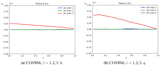
Figure 9. Test 4.1. Differences between the stationary and the numerical solutions for CLWBMi, $i=1,2,3$ at time $t=1$ s for a 200-cell mesh.

Table 14. Test 4.1. Differences in $L^1$-norm with respect to the stationary solution for CLWBMi ($i=1,2,3$) for the 200-cell mesh at time $t=1$ s.

Method	Error ($\mathit{i}=1$)		Error ($\mathit{i}=2$)		Error ($\mathit{i}=3$)
	$\mathit{h}$	$\mathit{q}$	$\mathit{h}$	$\mathit{q}$	$\mathit{h}$	$\mathit{q}$
CLWBMi	2.24 × ${10}^{-16}$	5.06 × ${10}^{-16}$	0.00	5.56 × ${10}^{-19}$	1.58 × ${10}^{-14}$	3.38 × ${10}^{-14}$

4.4.2. Test 4.2

Now, we consider a numerical experiment that corresponds to a small perturbation of the previous stationary solution $U^{*}\left(x\right)={[h^{*}\left(x\right),q^{*}\left(x\right)]}^T$:

$$h_0\left(x\right)=\left\{\begin{array}{cc}{h}^{*}\left(x\right)+0.2,\hfill & {\displaystyle \mathrm{if} \frac{3}{7}\le x\le \frac{4}{7},}\hfill \\ h^{*}\left(x\right),\hfill & \mathrm{otherwise},\hfill \end{array}\right.$$

$$q_0\left(x\right)=q^{*}\left(x\right).$$

As in Reference [47], we consider a mesh with 100 cells, and the model is run up to $t=9$ s.

As in the previous test case, only the well-balanced schemes will be considered. Figure 10 shows the discrepancies between the stationary and the numerical solutions for the water depth computed with CLWBMi, $i=1,2,3$ at the time steps $t=0.06$ s and $t=9$ s (the figures are similar for q). In black, we plot a reference solution computed with a 1st-order well-balanced scheme with a 1600-cell mesh.

Figure 10. Test 4.2. Reference and numerical solutions: differences with the stationary solution for CLWBMi, $i=1,2,3$, at times $t=0.06,9$ s for h on a 100-cell mesh.

As expected, the stationary solution is preserved by the well-balanced schemes after the perturbation left the domain. Table 15 shows the $L^1$ errors with respect to the steady state at $t=9$ s for 100-cell mesh.

Table 15. Test 4.2. Differences in $L^1$-norm with respect to the stationary solution for CLWBMi ($i=1,2,3$) for the 100-cell mesh at time $t=9$ s.

Method	Error ($\mathit{i}=1$)		Error ($\mathit{i}=2$)		Error ($\mathit{i}=3$)
	$\mathit{h}$	$\mathit{q}$	$\mathit{h}$	$\mathit{q}$	$\mathit{h}$	$\mathit{q}$
CLWBMi	2.99 × ${10}^{-16}$	3.97 × ${10}^{-16}$	1.81 × ${10}^{-15}$	2.76 × ${10}^{-15}$	6.50 × ${10}^{-14}$	1.77 × ${10}^{-14}$

4.4.3. Test 4.3

We end this subsection with two numerical experiments whose objective is show the efficiency of the schemes to preserve steady states that involve a varying bathymetry and friction. In this case, k takes the value of $0.01$ and the space domain is again the interval $[0,1]$. The bathymetry is given by

$${\displaystyle H\left(x\right)=1-\frac{1}{2}\frac{e^{cos\left(4\pi x\right)}-e^{-1}}{e-e^{-1}}.}$$

(75)

The first experiment concerns the preservation of the supercritical stationary solution corresponding to (72) with initial conditions $q\left(0\right)=1$ and $h\left(0\right)=0.3$.

Following Reference [47], we take 100 discretization cells, and the numerical simulation of this experiment is run until $t=1$ s.

Figure 11 shows the numerical solutions at $t=1$ s for NWBMi, $i=1,2,3$ and CLWBMi, $i=1,2,3.$ Notice that NWBM1 is completely wrong: due to the numerical diffusion, the supercritical regime is lost at the right side of the domain, which causes a shock wave traveling to the left (of course, this behavior disappears when the mesh is fine enough). Therefore, in Figure 12, where the differences with the stationary solution are plotted, only the results for NWBMi, $i=2,3$ and for CLWBMi, $i=1,2,3$ are shown. Table 16 shows the errors corresponding to the different methods for the 100-cell mesh. We also consider a reference solution computed with a well-balanced first order scheme on a 1600-cell mesh.

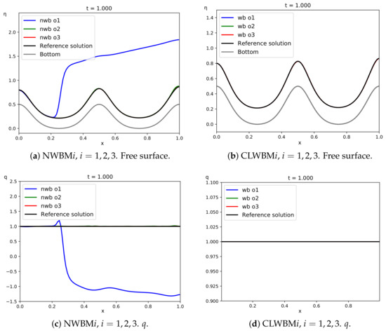
Figure 11. Test 4.3. 100-cell numerical solutions and reference solution at time $t=1$ s.

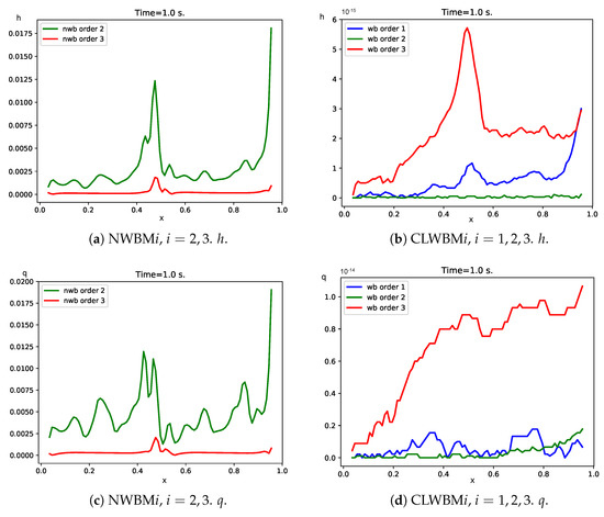
Figure 12. Test 4.3. Differences between the stationary and the numerical solutions at time $t=1$ s with a 100-cell mesh.

Table 16. Test 4.3. Differences in $L^1$-norm with respect to the stationary solution for NWBMi and CLWBMi ($i=1,2,3$) for the 100-cell mesh at time $t=1$ s.

Method	Error ($\mathit{i}=1$)		Error ($\mathit{i}=2$)		Error ($\mathit{i}=3$)
	$\mathit{h}$	$\mathit{q}$	$\mathit{h}$	$\mathit{q}$	$\mathit{h}$	$\mathit{q}$
NWBMi	8.28 × ${10}^{-1}$	1.54	3.61 × ${10}^{-3}$	4.88 × ${10}^{-3}$	3.65 × ${10}^{-3}$	4.30 × ${10}^{-4}$
CLWBMi	7.03 × ${10}^{-16}$	5.85 × ${10}^{-16}$	3.22 × ${10}^{-17}$	3.75 × ${10}^{-16}$	2.14 × ${10}^{-15}$	6.87 × ${10}^{-15}$

4.4.4. Test 4.4

Following Reference [47], the very last experiment in this subsection focuses on a perturbation of the aforementioned steady state. The initial condition $U_0\left(x\right)={[h_0\left(x\right),q_0\left(x\right)]}^T$ is given by:

$$h_0\left(x\right)=\left\{\begin{array}{cc}{h}^{*}\left(x\right)+0.05,\hfill & \mathrm{if} x\in \left[{\displaystyle \frac{2}{7},\frac{3}{7}}\right]\cup \left[{\displaystyle \frac{4}{7},\frac{5}{7}}\right],\hfill \\ h^{*}\left(x\right),\hfill & \mathrm{otherwise},\hfill \end{array}\right.$$

$$q_0\left(x\right)=\left\{\begin{array}{cc}{q}^{*}\left(x\right)+0.5,\hfill & \mathrm{if} x\in \left[{\displaystyle \frac{2}{7},\frac{3}{7}}\right]\cup \left[{\displaystyle \frac{4}{7},\frac{5}{7}}\right],\hfill \\ q^{*}\left(x\right),\hfill & \mathrm{otherwise},\hfill \end{array}\right.$$

where $U^{*}\left(x\right)={[h^{*}\left(x\right),q^{*}\left(x\right)]}^T$ is the stationary solution considered in the previous experiment. As in Reference [47], we use a 100-cell mesh for the numerical simulation on the domain $[0,1]$, and the computations are carried out until the final time $t=2$ s.

Observe that there are not big differences among the solutions during for small times. Nevertheless, for the NNWBM1, the supercritical regime is lost on the right of the domain, causing a shock traveling to the left, as in Test 4.3. Figure 13 shows then the differences between the numerical solutions and the stationary solution for h with NWBMi, $i=1,2,3$ at time $t=0.015$ and $i=2,3$ at time $t=2$, and with CLWBMi, $i=1,2,3$ at times $t=0.015$ and $t=2$ (the plots are similar for q). Again, in black, we plot a reference solution computed on a 1600-cell mesh with a first order well-balanced scheme.

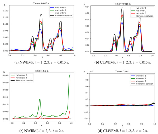
Figure 13. Test 4.4. Reference and numerical solutions: differences with the stationary solution at times $t=0.015,2$ s for h, for a 100-cell mesh.

Once more, well-balanced schemes are able to recover the stationary states after the perturbation left the domain. Table 17 shows the differences in $L^1$-norm with respect to the stationary solution at time $t=2$ s for a mesh with 100 cells.

Table 17. Test 4.4. Differences in $L^1$-norm with respect to the stationary solution for NWBMi and CLWBMi ($i=1,2,3$) at time $t=2$ s for a 100-cell mesh.

Method	Error ($\mathit{i}=1$)		Error ($\mathit{i}=2$)		Error ($\mathit{i}=3$)
	$\mathit{h}$	$\mathit{q}$	$\mathit{h}$	$\mathit{q}$	$\mathit{h}$	$\mathit{q}$
NWBMi	2.42	6.12	3.57 × ${10}^{-3}$	4.87 × ${10}^{-3}$	1.39 × ${10}^{-3}$	4.30 × ${10}^{-4}$
CLWBMi	3.73 × ${10}^{-16}$	3.60 × ${10}^{-16}$	1.80 × ${10}^{-15}$	1.99 × ${10}^{-15}$	2.64 × ${10}^{-15}$	8.93 × ${10}^{-15}$

4.5. Problem 5: Compressible Euler Equations with Gravitational Force

Finally, let us consider the compressible Euler equations for gas dynamics with gravity:

$$\left\{\begin{array}{c}{\rho }_t+{\left(\rho u\right)}_x=0,\hfill \\ {\left(\rho u\right)}_t+{\left(\rho u^2+p\right)}_x=-\rho H_x,\hfill \\ E_t+{\left(u(E+p)\right)}_x=-\rho u{H}_x.\hfill \end{array}\right.$$

(76)

Here, u is the velocity, $p\ge 0$ the pressure, $\rho \ge 0$ the density, $q=\rho u$ the momentum, E the total energy per unit volume, and $H\left(x\right)$ is the gravitational potential. The internal energy e is defined by ${\displaystyle \rho e=E-\frac{1}{2}\rho u^2}$, and pressure could be determined from the internal energy using the equation of state. In this work, we suppose an ideal gas; therefore,

$$p=(\gamma -1)\rho e,$$

(77)

$\gamma >1$ being the adiabatic constant. Here, it is set to $\gamma =1.5$.

Note that (76) is a particular case of (1) with $N=3$,

$$U=\left(\begin{array}{c}\rho \\ \rho u\\ E\end{array}\right),f\left(U\right)=\left(\begin{array}{c}\rho u\\ \rho u^2+p\\ u(E+p)\end{array}\right),S\left(U\right)=\left(\begin{array}{c}0\\ -\rho \\ -\rho u\end{array}\right).$$

Supposing that the system is strictly hyperbolic and considering (77), the stationary solutions satisfy the ODE system:

$$\left\{\begin{array}{c}{q}_x=0,\hfill \\ {\displaystyle \frac{d\widehat{U}}{dx}=G(x,\widehat{U}),}\hfill \end{array}\right.$$

(78)

where

$$\widehat{U}=\left(\begin{array}{c}\rho \\ E\end{array}\right),G(x,\widehat{U})=-\left(\begin{array}{c}{\displaystyle \frac{\rho }{c^2-u^2}}\\ {\displaystyle \frac{\rho }{\gamma -1}\left(1+\frac{3-\gamma }{2}\frac{u^2}{c^2-u^2}\right)}\end{array}\right)H_x,$$

where $c=\sqrt{\gamma p/\rho }$ is the sound speed, which is valid for stationary regular solution. Notice that, for regular solutions of the Euler equations, the entropy is constant along material lines. So that, for stationary solutions, $u{s}_x=0$, where s denotes the entropy density. Therefore, if u does not vanish, it follows that these stationary solutions are isentropic.

Test 5.1

In this test, we consider the space domain $[-1,1]$, and the system is integrated up to time $t=5$ s. The gravity potential is $H\left(x\right)=x$.

As initial condition, a supersonic stationary solution corresponding to the solution of the Cauchy problem

$$\left\{\begin{array}{c}{q}_x=0,\hfill \\ {\displaystyle \frac{d\widehat{U}}{dx}=G(x,\widehat{U}),}\hfill \\ \rho (-1)=1,q(-1)=10,E(-1)=52\hfill \end{array}\right.$$

(79)

is computed with the Gauss-Legendre collocation method. Density, momentum, and energy is set downstream, and open free boundary conditions upstream. $CFL$ parameter is set to $0.9$.

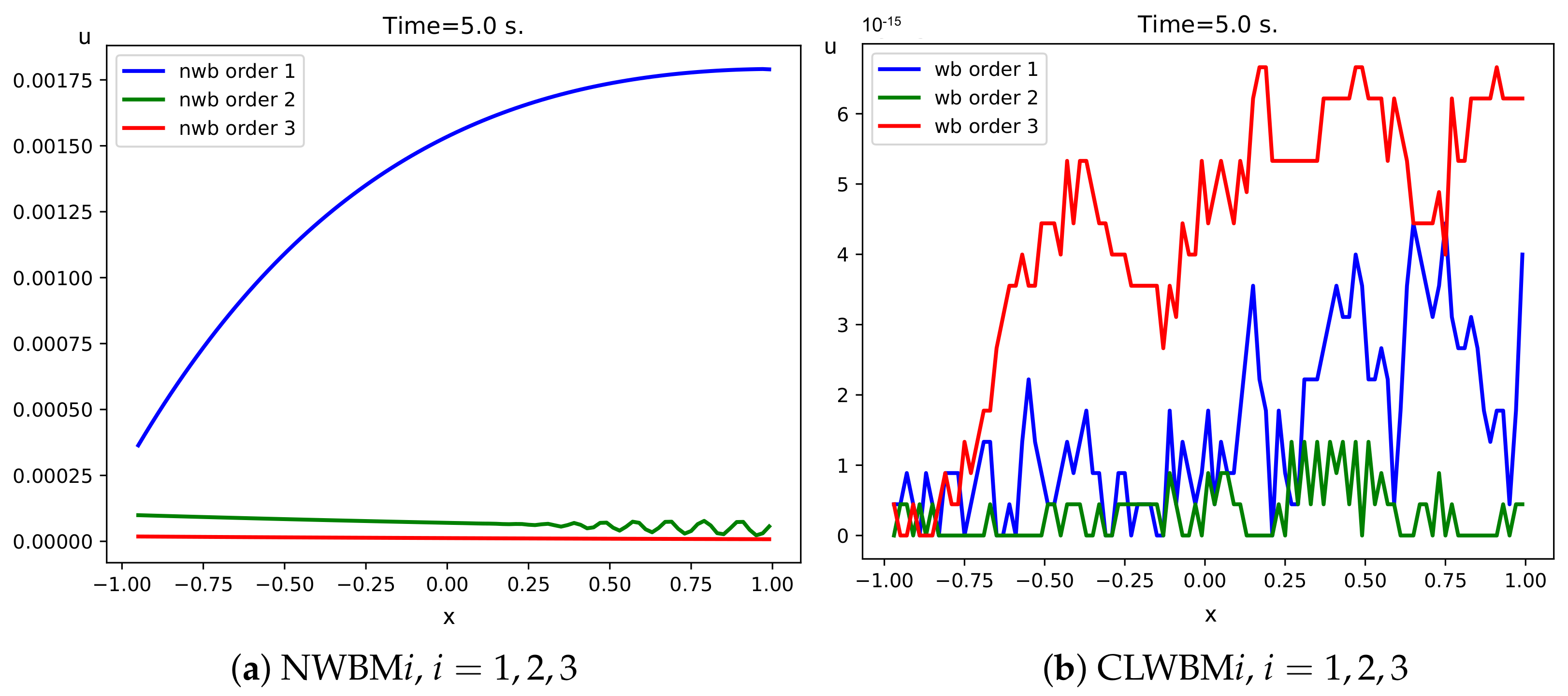
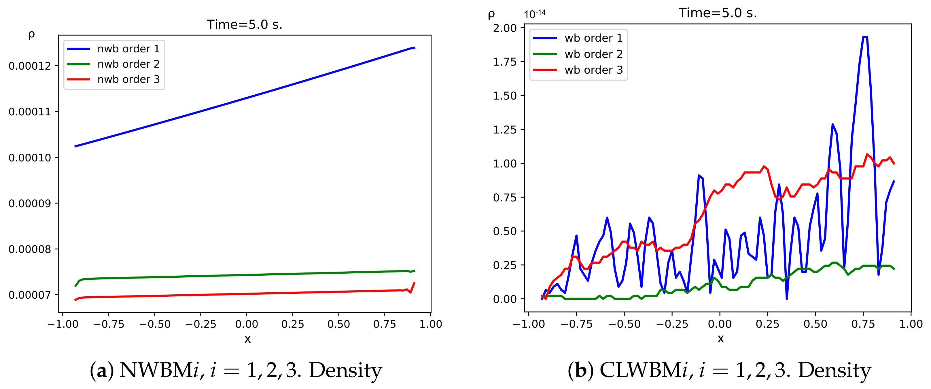
Figure 14, Figure 15 and Figure 16 show the differences between the stationary and the numerical solutions for NWBMi and CLWBMi, $i=1,2,3$ for $\rho$, q, and E, respectively; Table 18 shows the errors for for the 100-cell mesh with NWBMi and CLWBMi, $i=1,2,3$ at time $t=5$ s. Table 19 shows the computational cost for NWBMi, CWBMi, and CLWBMi, $i=1,2,3$. Notice that CLWBM are significantly more efficient than CWBM. We have carried out similar experiments with a perturbation of this stationary solution as initial condition, and we obtained the expected results, i.e., only the well-balanced methods are able to exactly recover the steady state solution. For the sake of conciseness, we do not present the tests here.

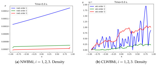
Figure 14. Test 5.1. Differences between the stationary and the numerical solutions at time $t=5$ s for $\rho$ with a mesh of 100 cells.

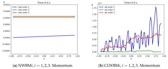
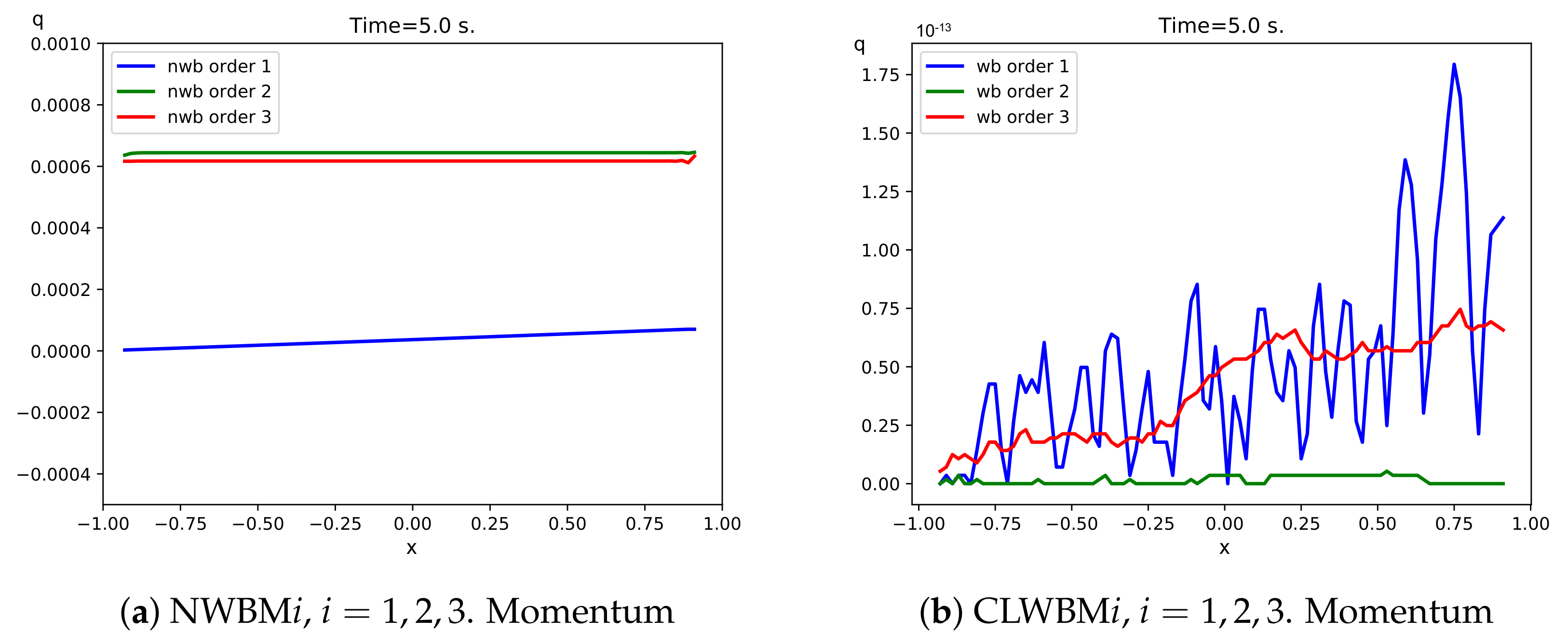
Figure 15. Test 5.1. Differences between the stationary and the numerical solutions at time $t=5$ s for q with a mesh of 100 cells.

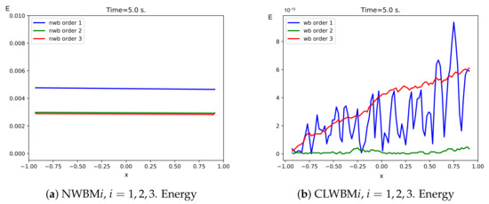
Figure 16. Test 5.1. Differences between the stationary and the numerical solutions at time $t=5$ s for E with a mesh of 100 cells.

Table 18. Test 5.1. Differences in $L^1$-norm with respect to the stationary solution for NWBMi and CLWBMi ($i=1,2,3$) for the mesh with 100 cells at time $t=5$ s.

Method	Error ($\mathit{i}=1$)	Error ($\mathit{i}=2$)	Error ($\mathit{i}=3$)
h
NWBMi	2.23 × ${10}^{-4}$	9.41 × ${10}^{-5}$	9.51 × ${10}^{-3}$
CLWBMi	6.97 × ${10}^{-15}$	6.58 × ${10}^{-14}$	3.20 × ${10}^{-13}$
q
NWBMi	1.45 × ${10}^{-4}$	1.28 × ${10}^{-3}$	5.95 × ${10}^{-3}$
CLWBMi	2.22 × ${10}^{-15}$	2.81 × ${10}^{-15}$	2.77 × ${10}^{-14}$
E
NWBMi	1.38 × ${10}^{-4}$	1.22 × ${10}^{-3}$	5.78 × ${10}^{-3}$
CLWBMi	1.24 × ${10}^{-14}$	8.13 × ${10}^{-14}$	7.15 × ${10}^{-13}$

Table 19. Test 5.1. Computational cost (milliseconds) for the mesh with 100 cells. $t=5$ s.

Order (i)	NWBMi	CWBMi	CLWBMi
1	120	4480	220
2	250	8960	1440
3	670	19430	4750

5. Conclusions

Following Reference [36], we propose a family of well-balanced high-order numerical schemes that can be applied to general 1D balance laws. Note that the main difficulty of the method proposed in Reference [36] comes from the fact that local stationary solutions must be computed at every cell that may require the knowledge of the stationary states. When solving the ODE (2) for the stationary solution is not possible or too costly, the first step has to be computed numerically: what we propose here is to build both the stationary solutions and the local solvers for the first step on the basis of the collocation RK methods. The well-balanced property of these numerical methods is precisely stated, and we have also introduced a general technique that allows us to deal with resonant problems for any 1D systems of balance laws.

We have considered a good number of examples: Burgers equation, shallow water system with friction, and Euler equations with gravity to check the well-balanced property of the methods and to test their efficiency. In some of these test cases, the stationary solutions are known either in implicit or explicit form, while, in others, the only information comes from the ODE (2) that the stationary solutions satisfy: in the former case, we can compare the efficiency of the new implementation, while, in the latter, we can show the generality of the methods.

Although well-balanced schemes are more costly, they are more effective than standard non-well-balanced methods when they are applied to the propagation of small perturbation around an equilibria or when long-time integration is required. Furthermore, the tests show that the strategy based on the collocation RK methods introduced in this work is more efficient than the one presented in Reference [39].

The methods considered here can be applied in principle to any system of balance laws. For instance, in the context of Euler equations, in Reference [48], a first and second order numerical scheme that is well-balanced for particular 1D radial solutions for the Euler equations in cylindrical coordinates has been developed following the strategy proposed by two of the authors that was later reviewed in Reference [37]. It is possible to use the technique described here to extend the methods in Reference [48] to more general source terms and higher-order. This will be considered in a future work.

Futher developments will include applications to:

• Balance laws (1) with non-regular source terms, that is systems for which H has jump discontinuities.
• Multidimensional problems.

References

- Audusse, E.; Bouchut, F.; Bristeau, M.O.; Klein, R.; Perthame, B. A fast and stable well-balanced scheme with hydrostatic reconstruction for shallow water flows. SIAM J. Sci. Comput. 2004, 25, 2050–2065. [Google Scholar] [CrossRef]
- Bouchut, F. Nonlinear Stability of Finite Volume Methods for Hyperbolic Conservation Laws: And Well-Balanced Schemes for Sources; Springer Science & Business Media: Berlin/Heidelberg, Germany, 2004. [Google Scholar]
- Castro, M.; Chacón Rebollo, T.; Fernández-Nieto, E.; Parés, C. On Well-Balanced Finite Volume Methods for Nonconservative Nonhomogeneous Hyperbolic Systems. SIAM J. Sci. Comput. 2007, 29, 1093–1126. [Google Scholar] [CrossRef] [Green Version]
- Chacón Rebollo, T.; Delgado, A.; Fernández-Nieto, E. A family of stable numerical solvers for the shallow water equations with source terms. Comput. Methods Appl. Mech. Eng. 2003, 192, 203–225. [Google Scholar] [CrossRef]
- Chacón Rebollo, T.; Delgado, A.; Fernández-Nieto, E. Asymptotically balanced schemes for non-homogeneous hyperbolic systems—Application to the Shallow Water equations. C. R. Math. 2004, 338, 85–90. [Google Scholar] [CrossRef]
- Varma, R.S.D.; Chandrashekar, P. A second-order well-balanced finite volume scheme for Euler equations with gravity. Comput. Fluids 2018, 181. [Google Scholar] [CrossRef] [Green Version]
- Chandrashekar, P.; Zenk, M. Well-Balanced Nodal Discontinuous Galerkin Method for Euler Equations with Gravity. J. Sci. Comput. 2015, 71. [Google Scholar] [CrossRef] [Green Version]
- Desveaux, V.; Zenk, M.; Berthon, C.; Klingenberg, C. A well-balanced scheme to capture non-explicit steady states in the Euler equations with gravity. Int. J. Numer. Methods Fluids 2016, 81, 104–127. [Google Scholar] [CrossRef]
- Desveaux, V.; Zenk, M.; Berthon, C.; Klingenberg, C. Well-balanced schemes to capture non-explicit steady states. RIPA model. Math. Comput. 2015, 85, 1. [Google Scholar] [CrossRef]
- Gosse, L. A well-balanced flux-vector splitting scheme designed for hyperbolic systems of conservation laws with source terms* 1. Comput. Math. Appl. 2000, 39, 135–159. [Google Scholar] [CrossRef] [Green Version]
- Gosse, L. A Well-Balanced Scheme Using Non-Conservative Products Designed for Hyperbolic Systems of Conservation Laws With Source Terms. Math. Model. Methods Appl. Sci. 1999, 11. [Google Scholar] [CrossRef] [Green Version]
- Gosse, L. Localization effects and measure source terms in numerical schemes for balance laws. Math. Comput. 2002, 71, 553–582. [Google Scholar] [CrossRef] [Green Version]
- Käppeli, R.; Mishra, S. Well-balanced schemes for the Euler equations with gravitation. J. Comput. Phys. 2014, 259, 199–219. [Google Scholar] [CrossRef]
- Greenberg, J.M.; LeRoux, A.Y. A well-balanced scheme for the numerical processing of source terms in hyperbolic equations. SIAM J. Numer. Anal. 1996, 33, 1–16. [Google Scholar] [CrossRef]
- Greenberg, J.; Leroux, A.; Baraille, R.; Noussair, A. Analysis and approximation of conservation laws with source terms. SIAM J. Numer. Anal. 1997, 34, 1980–2007. [Google Scholar] [CrossRef]
- LeVeque, R. Balancing source terms and flux gradients in high-resolution Godunov methods: The quasi-steady wave-propagation algorithm. J. Comput. Phys. 1998, 146, 346–365. [Google Scholar] [CrossRef] [Green Version]
- Lukacova-Medvidova, M.; Noelle, S.; Kraft, M. Well-balanced finite volume evolution Galerkin methods for the shallow water equations. J. Comput. Phys. 2007, 221, 122–147. [Google Scholar] [CrossRef] [Green Version]
- Noelle, S.; Pankratz, N.; Puppo, G.; Natvig, J. Well-balanced finite volume schemes of arbitrary order of accuracy for shallow water flows. J. Comput. Phys. 2006, 213, 474–499. [Google Scholar] [CrossRef]
- Noelle, S.; Xing, Y.; Shu, C.W. High-order well-balanced finite volume WENO schemes for shallow water equation with moving water. J. Comput. Phys. 2007, 226, 29–58. [Google Scholar] [CrossRef]
- Pelanti, M.; Bouchut, F.; Mangeney, A. A Roe-Type Scheme for Two-Phase Shallow Granular Flows over Variable Topography. ESAIM Math. Model. Numer. Anal. 2008, 42, 851–885. [Google Scholar] [CrossRef] [Green Version]
- Perthame, B.; Simeoni, C. A kinetic scheme for the Saint-Venant system with a source term. Calcolo 2001, 38, 201–231. [Google Scholar] [CrossRef]
- Perthame, B.; Simeoni, C. Convergence of the upwind interface source method for hyperbolic conservation laws. In Hyperbolic Problems: Theory, Numerics, Applications; Springer: Berlin/Heidelberg, Germany, 2003; pp. 61–78. [Google Scholar]
- Russo, G.; Khe, A. High order well balanced schemes for systems of balance laws. Proc. Symp. Appl. Math. 2009, 67, 919–928. [Google Scholar] [CrossRef]
- Tang, H.; Tang, T.; Xu, K. A gas-kinetic scheme for shallow-water equations with source terms. Z. Angew. Math. Phys. 2004, 55, 365–382. [Google Scholar] [CrossRef]
- Klingenberg, C.; Touma, R.; Koley, U. Well-Balanced Unstaggered Central Schemes for the Euler Equations with Gravitation. SIAM J. Sci. Comput. 2016, 38. [Google Scholar] [CrossRef]
- Xing, Y.; Shu, C.W. High order well-balanced finite volume WENO schemes and discontinuous Galerkin methods for a class of hyperbolic systems with source terms. J. Comput. Phys. 2006, 214, 567–598. [Google Scholar] [CrossRef]
- Klingenberg, C.; Puppo, G.; Semplice, M. Arbitrary Order Finite Volume Well-Balanced Schemes for the Euler Equations with Gravity. SIAM J. Sci. Comput. 2019, 41, A695–A721. [Google Scholar] [CrossRef] [Green Version]
- Kanbar, F.; Touma, R.; Klingenberg, C. Well-balanced Central Schemes for the One and Two-dimensional Euler Systems with Gravity. Appl. Numer. Math. 2020, 156. [Google Scholar] [CrossRef]
- Cheng, Y.; Kurganov, A. Moving-water equilibria preserving central-upwind schemes for the shallow water equations. Commun. Math. Sci. 2016, 14, 1643–1663. [Google Scholar] [CrossRef]
- Kurganov, A. Finite-volume schemes for shallow-water equations. Acta Numer. 2018, 27, 289–351. [Google Scholar] [CrossRef] [Green Version]
- Chertock, A.; Cui, S.; Kurganov, A.; Wu, T. Well-balanced positivity preserving central-upwind scheme for the shallow water system with friction terms. Int. J. Numer. Methods Fluids 2015, 78. [Google Scholar] [CrossRef] [Green Version]
- Castro, M.J.; de Luna, T.M.; Parés, C. Well-balanced schemes and path-conservative numerical methods. In Handbook of Numerical Analysis; Elsevier: Amsterdam, The Netherlands, 2017; Volume 18, pp. 131–175. [Google Scholar]
- Franck, E.; Mendoza, L.S. Finite volume scheme with local high order discretization of the hydrostatic equilibrium for the euler equations with external forces. J. Sci. Comput. 2016, 69, 314–354. [Google Scholar] [CrossRef] [Green Version]
- Grosheintz-Laval, L.; Käppeli, R. Well-balanced finite volume schemes for nearly steady adiabatic flows. J. Comput. Phys. 2020, 423, 109805. [Google Scholar] [CrossRef]
- Käppeli, R.; Mishra, S. A well-balanced finite volume scheme for the euler equations with gravitation-the exact preservation of hydrostatic equilibrium with arbitrary entropy stratification. Astron. Astrophys. 2016, 587, A94. [Google Scholar] [CrossRef] [Green Version]
- Castro, M.; Gallardo, J.; López-García, J.; Parés, C. Well-Balanced High Order Extensions of Godunov’s Method for Semilinear Balance Laws. SIAM J. Numer. Anal. 2008, 46, 1012–1039. [Google Scholar] [CrossRef]
- Castro, M.; Parés, C. Well-Balanced High-Order Finite Volume Methods for Systems of Balance Laws. J. Sci. Comput. 2020, 82. [Google Scholar] [CrossRef]
- Castro, M.; López-García, J.; Parés, C. High order exactly well-balanced numerical methods for shallow water systems. J. Comput. Phys. 2013, 246, 242–264. [Google Scholar] [CrossRef]
- Gómez-Bueno, I.; Castro, M.J.; Parés, C. High-order well-balanced methods for systems of balance laws: A control-based approach. Appl. Math. Comput. 2021, 394, 125820. [Google Scholar]
- Gómez-Bueno, I.; Castro, M.; Parés, C. Well-Balanced Reconstruction Operator for Systems of Balance Laws: Numerical Implementation. In Recent Advances in Numerical Methods for Hyperbolic PDE Systems; Springer: Berlin/Heidelberg, Germany, 2021; pp. 57–77. [Google Scholar]
- Bermudez, A.; Vazquez, M.E. Upwind methods for hyperbolic conservation laws with source terms. Comput. Fluids 1994, 23, 1049–1071. [Google Scholar] [CrossRef]
- Haier, E.; Lubich, C.; Wanner, G. Geometric Numerical Integration: Structure-Preserving Algorithms for Ordinary Differential Equations; Springer: Berlin/Heidelberg, Germany, 2006. [Google Scholar]
- Van Leer, B. Towards the Ultimate Conservative Difference Scheme V. A Second-order Sequel to Godunov’s Method. J. Comput. Phys. 1979, 32, 101–136. [Google Scholar] [CrossRef]
- Levy, D.; Puppo, G.; Russo, G. Compact Central WENO Schemes for Multidimensional Conservation Laws. SIAM J. Sci. Comput. 2000, 22. [Google Scholar] [CrossRef] [Green Version]
- Cravero, I.; Semplice, M. On the accuracy of WENO and CWENO reconstructions of third order on nonuniform meshes. J. Sci. Comput. 2015, 67. [Google Scholar] [CrossRef] [Green Version]
- Gottlieb, S.; Shu, C.W. Total Variation Diminishing Runge-Kutta Schemes. Math. Comput. 1996, 67. [Google Scholar] [CrossRef] [Green Version]
- Michel-Dansac, V.; Berthon, C.; Clain, S.; Foucher, F. A well-balanced scheme for the shallow-water equations with topography. Comput. Math. Appl. 2015, 72. [Google Scholar] [CrossRef] [Green Version]
- Gaburro, E.; Castro, M.J.; Dumbser, M. Well-balanced Arbitrary-Lagrangian-Eulerian finite volume schemes on moving nonconforming meshes for the Euler equations of gas dynamics with gravity. Mon. Not. R. Astron. Soc. 2018, 477, 2251–2275. [Google Scholar] [CrossRef] [Green Version]
Publisher’s Note: MDPI stays neutral with regard to jurisdictional claims in published maps and institutional affiliations. |
© 2021 by the authors. Licensee MDPI, Basel, Switzerland. This article is an open access article distributed under the terms and conditions of the Creative Commons Attribution (CC BY) license (https://creativecommons.org/licenses/by/4.0/).