Optimal Control of Dengue Transmission with Vaccination

Abstract

Dengue disease is caused by four serotypes of the dengue virus: DEN-1, DEN-2, DEN-3, and DEN-4. The chimeric yellow fever dengue tetravalent dengue vaccine (CYD-TDV) is a vaccine currently used in Thailand. This research investigates what the optimal control is when only individuals having documented past dengue infection history are vaccinated. This is the present practice in Thailand and is the latest recommendation of the WHO. The model used is the Susceptible-Infected-Recovered (SIR) model in series configuration for the human population and the Susceptible-Infected (SI) model for the vector population. Both dynamical models for the two populations were recast as optimal control problems with two optimal control parameters. The analysis showed that the equilibrium states were locally asymptotically stable. The numerical solution of the control systems and conclusions are presented.

1. Introduction

The dengue epidemic first occurred in the Philippines in 1954. It reached Thailand in 1958. The disease is caused by an infection by any one of the four serotypes of dengue virus, which are labeled as DEN-1, DEN-2, DEN-3, and DEN-4. The dengue viruses are transmitted by two species of the Aedes mosquitoes, the Aedes aegypti and the Aedes albopictus. All four serotypes have a common antigen, resulting in cross-reaction and cross-protection of the four serotypes. The cross protection is not permanent. A person infected by one of the serotypes will have permanent immunity to that serotype, but only partial immunity to the other three. Some of the immunity will last for a short period, approximately 6–12 months. Those people might be re-infected if they happen to meet a different serotype of dengue virus. This second infection is different from the initial infection and is labeled as a secondary dengue infection [1,2,3,4] since the symptoms and outcomes of the primary and secondary dengue infections can be quite different. In some individuals (infants or young children), infection by the dengue virus may lead to undifferentiated fever (uf). The individuals are said to have the viral syndrome of dengue fever, which can only be detected through laboratory tests. In older children and adults, infection by the dengue viruses leads to what is usually labeled as dengue fever (DF). People with DF exhibit symptoms such a mild fever, headaches, pain around the eyes, muscular pain, and pain in the bones. If an individual experiences the clinical symptoms of high fever accompanied by bleeding, enlarged liver, and severe shock, he is said to have dengue hemorrhagic fever (DHF). During the fever, there will also be a low platelet count and plasma leakage. If large amounts of plasma leak out, the patient will have a shock condition called dengue shock syndrome (DSS) [5,6,7]. The last two (DHF and DSS) are the symptoms that the individuals in the secondary dengue infection group experience. These symptoms can be viewed as an allergic reaction.

Since millions of people can be infected by the dengue virus, there is an economic cost to these people becoming sick, and vaccines have been developed. Chimeric yellow fever dengue tetravalent dengue vaccine (CYD-TDV) is one of these vaccines. It was first registered as a dengue vaccine in Mexico. It is now registered in 13 countries around the world, including Thailand, which had a role in its development. This dengue vaccine is the first and only vaccine in the world at the moment to cover all four strains of the dengue virus and is called Dengvaxia^®, which is developed by Sanofi Pasteur to help protect against the dengue disease. The vaccine has an overall effectiveness of 56.5%, which is 74% more effective in older children, 12–14 years old, and 75% effective for DEN-3 and DEN-4 [8,9]. It is reported that the efficacy of the vaccine is higher in children who have previously been infected with dengue fever. The dengue vaccine reduces the severity of the disease by 88.5% and hospitalization by 67.2% [10,11,12]. In December 2017, the WHO [13] issued a new recommendation that states that the WHO recommends vaccination (with Dengvaxia) only in individuals with a documented past dengue infection. This should be taken into consideration in any models used.

Esteva and Vargas [4,14] were among the first to study the transmission of dengue disease. They developed a mathematical model in which there were compartmental models for both the human and mosquito populations. The human population was described by a Susceptible-Infected-Recovered (SIR) model while the mosquito population was described by an SI (no recovered) model. Pongsumpun et al. [15,16,17] have also studied the transmission of dengue virus. Most of Pongsumpun’s work has been centered on the situation in Thailand since the dengue fever is of major concern to Thailand. She has included an exposed class (E) to the model, making the Susceptible-Infected-Exposed-Recovered (SEIR) model, to describe the dynamics of the human population. In Ref. [16], the author used the SIR model to simulate the possible outcomes of vertical transmission of the virus among mosquitos. She and her coworkers [17] included vertical transmission in a SEIR model. Syafruddin and Noorani [18] studied the mathematical model for dengue transmission and applied it to the situations in Indonesia and Malaysia. Yaacob [19] studied the mathematical model of the dengue disease in people who have no immunity.

Singh et al. [20] and Tasman et al. [21] considered the effects of vaccination on a model in which the human population is divided into children and adults. They also considered that there were two types of infections, primary and secondary dengue infection. It was assumed that individuals experiencing a secondary infection were at a higher risk. In these studies, the adults were further divided in two groups, so the human population consisted to three groups: less than 9 years, between 9 and 45 years, and between 45 and 65 years [22,23]. Using a similar model to study the transmission of another disease, melioidosis, Tavaen and Viriyapong [24] studied the local and global stability analyses and optimal control for this disease. There are many studies about the effects of the dengue vaccination on the spread of the dengue disease. [25,26,27,28]. They have introduced various models to simulate the dynamic of the programs when there is complete vaccination, random mass vaccination, imperfect random mass vaccination, and random mass vaccination with waning immunity levels. They have used optimal control strategies to simulate the results of the programs.

The number of cases and deaths by month and the number of cases and deaths each year in Thailand from 2003–2020 data from the Bureau of Epidemiology at the Ministry of Health is shown in Figure 1. It can be seen in the figure that the dengue fever is prevalent in the rainy season from June to September. The incidence is the highest in July. The number of cases, which fluctuated month to month, tended to increase yearly from 2003 to 2020. The same is true for the number of deaths. When the number of cases is high, there will be more deaths. The percentage of deaths is very small. Using the sources that gave these results, we were interested in the outcome of a vaccination program in which only individuals with a documented past dengue infection (i.e., an individual who would have a secondary dengue infection if bitten by a mosquito infected with a different serotype of the virus) are vaccinated. We used the double Susceptible-Infected-Recovered (SIR) model for the human population and the Susceptible-Infected (SI) model for the vector population. The analysis of the stability of the model was carried out by using dynamic analysis. The Routh–Hurwitz criteria were applied to analyze the system model for stability. The reproductive number was calculated. The optimal control theory was applied in the transmission model in order to minimize the number of infected humans with primary and secondary infections. Numerical simulation was performed. Results and conclusion are presented in this paper.

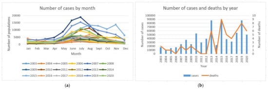
Figure 1. The number of cases by month and the number of cases and deaths each year from 2003–2020 [29]: (a) the number of cases by month; (b) the number of cases and deaths by year.

2. Materials and Methods

2.1. Mathematical Model

The basic mathematical model was the SEIR model presented in ref. [15]. The equations in that model describe the dynamics of the spread of dengue fever when there is only one serotype of the virus present. In this work, the basic SEIR model of [15] was extended to include secondary infection of a different serotype, whereby the members of the recovered population become the susceptible members in the second SIR, effectively providing a framework for describing a vaccination program in which only people who have been infected are considered. In Thailand, the medical status of each Thai citizen is kept at the District Office in each province in the country. It is easy to determine from the past medical histories anyone who was infected with the dengue virus. Dengue fever is one of the five diseases that must be reported to the Thai Ministry of Health. The susceptible human population in the second SIR model used here are the not sick humans who have been infected by the serotype A virus, since they will be the only ones given the vaccine. A person who has no prior history of any dengue infection is not considered to be a candidate for the vaccination. The vector population was divided into two compartments: susceptible and infected (SI). The infected mosquito was the subset of infected mosquitoes transmitting virus B. The human population was subdivided into six population groups. It should be remembered that all of the recovered individuals have the antibodies to a particular serotype of the dengue virus at the end of primary infection. Susceptible people of this kind are not born into this group; they emerge after several months of being infected by a serotype virus. The vector population was classified into two subclasses. The variables are defined in Table 1.

Table 1. The definition of the variables used in the differential system of Equations (1)–(10).

Variables	Definition
$\overline{S_{HP}}$	The number of humans susceptible to primary infection
$\overline{I_{HP}}$	The number of humans with a primary infection
$\overline{R_{HP}}$	The number of humans who have recovered from a primary infection
$\overline{S_{HS}}$	The number of humans susceptible to secondary infection
$\overline{I_{HS}}$	The number of humans with a secondary infection
$\overline{R_{HS}}$	The number of humans who have recovered from a secondary infection
$\overline{S_V}$	The number of susceptible vectors
$\overline{I_V}$	The number of infected vectors

The dynamic transmission of dengue disease with the vaccination model is shown in Figure 2.

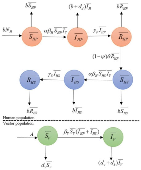
Figure 2. Diagram of the transmission model of dengue disease with the vaccination model of human and vector populations.

The dynamics of human and vector populations and the system of differential equations are given by:

$$\frac{d\overline{S_{HP}}}{dt}=b{N}_H-\alpha {\beta }_H\overline{S_{HP}}\overline{I_V}-b\overline{S_{HP}}$$

(1)

$$\frac{d\overline{I_{HP}}}{dt}=\alpha {\beta }_H\overline{S_{HP}}\overline{I_V}-{\gamma }_P\overline{I_{HP}}-\left(b+d_d\right)\overline{I_{HP}}$$

(2)

$$\frac{d\overline{R_{HP}}}{dt}={\gamma }_P\overline{I_{HP}}-\left(1-\psi \right)\theta \overline{R_{HP}}-b\overline{R_{HP}}$$

(3)

$$\frac{d\overline{S_{HS}}}{dt}=\left(1-\psi \right)\theta \overline{R_{HP}}-\alpha {\beta }_H\overline{S_{HS}}\overline{I_V}-b\overline{S_{HS}}$$

(4)

$$\frac{d\overline{I_{HS}}}{dt}=\alpha {\beta }_H\overline{S_{HS}}\overline{I_V}-{\gamma }_P\overline{I_{HS}}-b\overline{I_{HS}}$$

(5)

$$\frac{d\overline{R_{HS}}}{dt}={\gamma }_S\overline{I_{HS}}-b\overline{R_{HS}}$$

(6)

$$\frac{d\overline{S_V}}{dt}=A-{\beta }_V\overline{S_V}\left(\overline{I_{HP}}+\overline{I_{HS}}\right)-d_V\overline{S_V}$$

(7)

$$\frac{d\overline{I_V}}{dt}={\beta }_V\overline{S_V}\left(\overline{I_{HP}}+\overline{I_{HS}}\right)-\left(d_V+d_k\right)\overline{I_V}$$

(8)

with the conditions:

$$\overline{S_{HP}}+\overline{I_{HP}}+\overline{R_{HP}}+\overline{S_{HS}}+\overline{I_{HS}}+\overline{R_{HS}}=N_H$$

(9)

$$\overline{S_V}+\overline{I_V}=N_V$$

(10)

where the parameters of Equations (1)–(10) are defined in Table 2.

Table 2. The definition of the parameters of the differential system of Equations (1)–(10).

Parameters	Definition
$\alpha$	The biting rate of the vector population
$\psi$	The vaccine efficiency
$\theta$	The recurrent infection rate
$N_H$	The total number of humans in the study population
$N_V$	The total number of vectors in the study population
${\beta }_H$	The transmission rate of dengue virus from vector to human
${\beta }_V$	The transmission rate of dengue virus from human to vector
$b$	The birth and natural mortality rate of the human population
$d_V$	The natural mortality rate of the vector population
$d_d$	The mortality rate from infection of the human population
$d_k$	The mortality rate from infection of the vector population
${\gamma }_P$	The recovery rate of those with a primary infection
${\gamma }_S$	The recovery rate of those with a secondary infection

The rate of change of both the total population of humans and vectors is zero and given by:

$$\frac{d\overline{S_{HP}}}{dt}+\frac{d\overline{I_{HP}}}{dt}+\frac{d\overline{R_{HP}}}{dt}+\frac{d\overline{S_{HS}}}{dt}+\frac{d\overline{I_{HS}}}{dt}+\frac{d\overline{R_{HS}}}{dt}=0$$

(11)

$$\frac{d\overline{S_V}}{dt}+\frac{d\overline{I_V}}{dt}=0$$

(12)

with conditions, we get:

$$d_d\overline{I_{HP}}=0$$

(13)

$$d_k\overline{I_V}+d_V{N}_V=A$$

(14)

Normalizing the equations by introducing the following normalized variables:

$$S_{HP}=\frac{\overline{S_{HP}}}{N_H}, I_{HP}=\frac{\overline{I_{HP}}}{N_H}, R_{HP}=\frac{\overline{R_{HP}}}{N_H},S_{HS}=\frac{\overline{S_{HS}}}{N_H}, I_{HS}=\frac{\overline{I_{HS}}}{N_H}, R_{HS}=\frac{\overline{R_{HS}}}{N_H}$$

(15)

$$S_V=\frac{\overline{S_V}}{N_V}, I_V=\frac{\overline{I_V}}{N_V}$$

(16)

with the additional condition:

$$S_{HP}+ I_{HP}+R_{HP}+S_{HS}+ I_{HS}+R_{HS}=1$$

(17)

$$S_V+I_V=1$$

(18)

The mathematical model of Equations (1)–(8) is now reduced to the following equation:

$$\frac{d{S}_{HP}}{dt}=b-\alpha {\beta }_H{S}_{HP}{I}_V{N}_V-b{S}_{HP}$$

(19)

$$\frac{d{I}_{HP}}{dt}=\alpha {\beta }_H{S}_{HP}{I}_V{N}_V-{\gamma }_P{I}_{HP}-\left(b+d_d\right)I_{HP}$$

(20)

$$\frac{d{R}_{HP}}{dt}={\gamma }_P{I}_{HP}-\left(1-\psi \right)\theta R_{HP}-b{R}_{HP}$$

(21)

$$\frac{d{S}_{HS}}{dt}=\left(1-\psi \right)\theta R_{HP}-\alpha {\beta }_H{S}_{HS}{I}_V{N}_V-b{S}_{HS}$$

(22)

$$\frac{d{I}_{HS}}{dt}=\alpha {\beta }_H{S}_{HS}{I}_V{N}_V-{\gamma }_S{I}_{HS}-b{I}_{HS}$$

(23)

$$\frac{d{I}_V}{dt}={\beta }_V\left(1-I_V\right)\left(I_{HP}+I_{HS}\right)N_H-\left(d_V+d_k\right)I_V$$

(24)

2.2. The Equilibrium Points

Definition 1

([17]). The point $\tilde{X}\in {ℝ}^n$ is an equilibrium point for the differential equation $\frac{dX}{dt}=f\left(t,X\right)$ if $f\left(t,\tilde{X}\right)=0$ for all $t$.

Since epidemiological models are inherently dynamical systems, the knowledge of the equilibrium points is vital for determining the behavior of long-term dynamics. Towards this goal, the most important parameter for determining whether an outbreak will occur or not is the basic reproductive number $R_0$. The equilibrium points are obtained by setting the right-hand side of Equations (19)–(24) to zero. This system model now admits two equilibrium points, namely the disease-free point and an endemic equilibrium point. The disease-free equilibrium point $E_1$ is:

$$E_1=\left(1,0,0,0,0,0\right)$$

(25)

The endemic equilibrium point $E_2=\left(S_{HP}^{*},I_{HP}^{*},R_{HP}^{*},S_{HS}^{*},I_{HS}^{*},I_V^{*}\right)$ is:

$$\begin{gathered} S_{HP}^{*}=\frac{{\tau }_1\left(b\left(2\theta \left(\psi -1\right){\gamma }_P\right)-{\tau }_2\right)-{\tau }_7+\sqrt{{\tau }_3\left({\tau }_4+{\tau }_5\right)+{\tau }_7^2}}{{\tau }_6} \\ {I}_{HP}^{*}=\frac{b{\tau }_1{\tau }_2+{\tau }_7-\sqrt{{\tau }_3\left({\tau }_4+{\tau }_5\right)+{\tau }_7^2}}{{\tau }_6} \\ {R}_{HP}^{*}=\frac{b{\tau }_1{\tau }_2+{\tau }_7+\sqrt{{\tau }_3\left({\tau }_4+{\tau }_5\right)+{\tau }_7^2}}{{\tau }_6} \\ {S}_{HS}^{*}=\frac{{\tau }_7+\left({\tau }_3-{\tau }_{25}+{\tau }_{26}\right)\sqrt{{\tau }_3\left({\tau }_4+{\tau }_5\right)+{\tau }_7^2}+{\tau }_{22}}{{\tau }_{18}{\tau }_{19}{\tau }_{20}{\tau }_{21}} \\ {I}_{HS}^{*}=\frac{{\tau }_7+\left({\tau }_3-{\tau }_{25}+{\tau }_{26}\right)\sqrt{{\tau }_3\left({\tau }_4+{\tau }_5\right)+{\tau }_7^2}-{\tau }_{22}}{{\tau }_{18}{\tau }_{19}{\tau }_{20}{\tau }_{21}} \\ {I}_V^{*}=\frac{\sqrt{{\tau }_3\left({\tau }_4+{\tau }_5\right)+{\tau }_7^2}-{\tau }_{22}-{\tau }_7}{{\tau }_{27}+{\tau }_{28}} \end{gathered}$$

(26)

where:

$$\begin{gathered} {\tau }_1=b\alpha N_H{N}_V{\beta }_H{\beta }_V, {\tau }_2=\left(b+\theta -\theta \psi \right)\left(b+{\gamma }_S\right), {\tau }_3=b^2{\alpha }^2{N}_H{N}_V^2{\beta }_H^2{\beta }_V, \\ {\tau }_4=4\theta \left(\psi -1\right)\left(d_V+d_k\right)\left(b+\alpha N_V{\beta }_H\right)\left(b+d_d+{\gamma }_P\right){\gamma }_P{\tau }_2, \\ {\tau }_5=N_H{\beta }_{V}b{\tau }_2, {\tau }_6=2\alpha \theta \left(\psi -1\right)N_H{N}_V{\beta }_H\left(b+\alpha N_V{\beta }_H\right){\beta }_V{\gamma }_P\left(b+d_d+{\gamma }_P\right), \\ {\tau }_7=\alpha N_V{\beta }_H\left(\theta \left(\psi -1\right){\gamma }_P\right)+{\tau }_2, {\tau }_8=2\left(b+d_d+{\gamma }_P\right){\tau }_2, \\ {\tau }_9=2b^2\alpha \theta \left(\psi -1\right)\left(d_V+d_k\right)N_V{\beta }_H{\gamma }_P, \\ {\tau }_{10}=2b{\alpha }^2{\theta }^2{\left(\psi -1\right)}^2\left(d_V+d_k\right)N_V^2{\beta }_H^2{\gamma }_P\left(d_d+{\gamma }_P\right){\gamma }_S, \\ {\tau }_{11}=\theta -\theta \psi +d_d+\alpha N_V{\beta }_H+{\gamma }_P+{\gamma }_S, \\ {\tau }_{12}=\theta \left(\psi -1\right)\left({\gamma }_P+d_d\right)-\alpha N_V{\beta }_H-{\gamma }_S, \\ {\tau }_{13}=\left(\theta \left(\psi -1\right)-{\gamma }_P-{\gamma }_S\right)\left(\alpha N_V{\beta }_H+1\right), \\ {\tau }_{14}=\alpha \theta \left(\psi -1\right)N_V{\beta }_H\left(d_d+{\gamma }_P\right), {\tau }_{15}=d_d\left(\theta \left(\psi -1\right)-\alpha N_V{\beta }_H\right), \\ {\tau }_{16}={\left(2b\alpha N_V{\beta }_H\left(\theta -\theta \psi \right){\gamma }_P+\left(b+\theta -\theta \psi \right)\left(b+{\gamma }_S\right)\right)}^2, \\ {\tau }_{17}=b^2\left(2{\theta }^2{\left(\psi -1\right)}^2{\gamma }_P^2-2\theta \left(\psi -1\right){\gamma }_P{\tau }_2+{\tau }_2^2\right), \\ {\tau }_{18}=4b^2{\alpha }^2\theta \left(\psi -1\right)\left(b+\theta -\theta \psi \right)N_H{N}_V^2{\beta }_H^2{\left(b+\alpha N_V{\beta }_H\right)}^2, {\tau }_{19}={\beta }_V{\gamma }_P\left(b+d_d+{\gamma }_P\right), \\ {\tau }_{20}={\tau }_2\left(d_k\left(b+d_d+{\gamma }_P\right)-d_V\left(b+d_d+{\gamma }_P\right)+1\right), {\tau }_{21}=b{N}_H{\beta }_V\left(\theta -\theta \psi \right){\gamma }_P, \\ {\tau }_{22}=b\alpha N_V{\beta }_H{\tau }_8\left(d_V+d_k\right)+N_H{\beta }_{V}b{\tau }_7, \\ {\tau }_{23}={\tau }_9\left(b^3+b^2{\tau }_{11}-b{\tau }_{12}-{\tau }_{14}{\tau }_{15}\right)-{\tau }_{10}+{\tau }_{13}+{\tau }_1{\tau }_{16}{\tau }_{17}, \\ {\tau }_{24}=b^2\left(\theta \psi -\alpha N_V{\beta }_H+{\gamma }_S\right)+b\alpha \theta N_V{\beta }_H\left(\psi -1\right), \\ {\tau }_{25}=\theta \left(\psi +1\right)\left(2b\theta {\gamma }_S+\alpha N_V{\beta }_H{\gamma }_P+b{\gamma }_S\right), \\ {\tau }_{26}=N_V{\beta }_H{\gamma }_S\left(\alpha \theta \psi -b\alpha -\alpha \theta \right)+b^2\left(1+b\right), \\ {\tau }_{27}=2{\alpha }^2{N}_V^2{\beta }_H^2\left(d_V+d_k\right){\tau }_8, {\tau }_{28}=b{N}_H{\beta }_V\left(\theta -\theta \psi \right){\gamma }_P+{\tau }_2 \end{gathered}$$

2.3. The Basic Reproductive Number

Definition 2

([24]). Basic reproductive number ($R_0$) is defined as the average number of secondary infections when a single infective enters an entirely susceptible population.

The basic reproductive number ($R_0$) is obtained using the next-generation matrix method [30,31,32]. We selected $I_{HP},I_{HS},$ and $I_V$ to be the classes to construct the $F$ and $V$ matrices, which are important to this method. For our system, the matrices $F$ and $V$ contain new infection terms and transition terms. We evaluated the Jacobian matrices $F$ and $V$ at the disease-free equilibrium point $E_1=\left(1,0,0,0,0,0\right)$, where $F$ is non-negative and $V$ is non-singular. The $F$ (gains) and $V$ (losses) matrices are:

$$F=\left[\begin{array}{ccc}\frac{\partial f_1}{\partial I_{HP}}\left(E_1\right)& \frac{\partial f_1}{\partial I_{HS}}\left(E_1\right)& \frac{\partial f_1}{\partial I_V}\left(E_1\right)\\ \frac{\partial f_2}{\partial I_{HP}}\left(E_1\right)& \frac{\partial f_2}{\partial I_{HS}}\left(E_1\right)& \frac{\partial f_2}{\partial I_V}\left(E_1\right)\\ \frac{\partial f_3}{\partial I_{HP}}\left(E_1\right)& \frac{\partial f_3}{\partial I_{HS}}\left(E_1\right)& \frac{\partial f_3}{\partial I_V}\left(E_1\right)\end{array}\right], V=\left[\begin{array}{ccc}\frac{\partial v_1}{\partial I_{HP}}\left(E_1\right)& \frac{\partial v_1}{\partial I_{HS}}\left(E_1\right)& \frac{\partial v_1}{\partial I_V}\left(E_1\right)\\ \frac{\partial v_2}{\partial I_{HP}}\left(E_1\right)& \frac{\partial v_2}{\partial I_{HS}}\left(E_1\right)& \frac{\partial v_2}{\partial I_V}\left(E_1\right)\\ \frac{\partial v_3}{\partial I_{HP}}\left(E_1\right)& \frac{\partial v_3}{\partial I_{HS}}\left(E_1\right)& \frac{\partial v_3}{\partial I_V}\left(E_1\right)\end{array}\right]$$

where:

$$f=\left[\begin{array}{c}{f}_1\\ f_2\\ f_3\end{array}\right]=\left[\begin{array}{c}\alpha {\beta }_H{S}_{HP}{I}_V{N}_V\\ \alpha {\beta }_H{S}_{HS}{I}_V{N}_V\\ {\beta }_V\left(I_{HP}+I_{HS}\right)N_H\end{array}\right] , v=\left[\begin{array}{c}{v}_1\\ v_2\\ v_3\end{array}\right]=\left[\begin{array}{c}\left({\gamma }_P+b+d_d\right)I_{HP}\\ \left({\gamma }_S+b\right)I_{HS}\\ \left(d_V+d_k\right)I_V\end{array}\right]$$

The required matrices are:

$$\begin{gathered} F=\left[\begin{array}{ccc}0& 0& \alpha {\beta }_H{N}_V\\ 0& 0& 0\\ {\beta }_V{N}_H& {\beta }_V{N}_H& 0\end{array}\right], V=\left[\begin{array}{ccc}{\gamma }_P+b+d_d& 0& 0\\ 0& {\gamma }_S+b& 0\\ 0& 0& d_V+d_k\end{array}\right] \\ {V}^{-1}=\left[\begin{array}{ccc}\frac{1}{{\gamma }_P+b+d_d}& 0& 0\\ 0& \frac{1}{{\gamma }_S+b}& 0\\ 0& 0& \frac{1}{d_V+d_k}\end{array}\right] \end{gathered}$$

Since $R=F{V}^{-1}$, we have:

$$R=\left[\begin{array}{ccc}0& 0& \frac{\alpha N_V{\beta }_H}{d_V+d_k}\\ 0& 0& 0\\ \frac{N_H{\beta }_V}{b+d_d+{\gamma }_P}& \frac{N_H{\beta }_V}{b+{\gamma }_S}& 0\end{array}\right]$$

$R_0$ is the dominant eigenvalue of the matrix $R;$ then, the value of the basic reproductive number is given by:

$$R_0=\sqrt{\frac{\alpha N_H{N}_V{\beta }_H{\beta }_V}{d_k\left(b+d_d\right)+d_V\left(b+d_d\right)+{\gamma }_P\left(d_V+d_k\right)}}$$

(27)

2.4. Local Stability of Equilibrium Points

Definition 3

([14]). The equilibrium point $E_0$ of the system $\dot{X}=f\left(X\right)$ is locally asymptotically stable if the matrix $J=\frac{\partial f}{\partial X}\left(E_0\right)$ has all its eigenvalues with negative real parts. The equilibrium point $E_0$ is not stable if at least one of the eigenvalues of the matrix $J$ has a positive real part.

The local stability of each equilibrium point states of this model is determined from the Jacobian matrix at that equilibrium point of the system of Equations (19)–(24). The Jacobian matrix is:

$$J_{E_i}=\left[\begin{array}{cccccc}-\alpha {\beta }_H{I}_V{N}_V-b& 0& 0& 0& 0& -\alpha {\beta }_H{S}_{HP}{N}_V\\ \alpha {\beta }_H{I}_V{N}_V& -{\gamma }_P-d_d-b& 0& 0& 0& \alpha {\beta }_H{S}_{HP}{N}_V\\ 0& {\gamma }_P& -(1-\psi )\theta -b& 0& 0& 0\\ 0& 0& (1-\psi )\theta & -\alpha {\beta }_H{I}_V{N}_V-b& 0& -\alpha {\beta }_H{S}_{HS}{N}_H\\ 0& 0& 0& \alpha {\beta }_H{I}_{V}N& -{\gamma }_S-b& \alpha {\beta }_H{S}_{HS}{N}_H\\ 0& {\beta }_V{N}_H(1-I_V)& 0& 0& {\beta }_V{N}_H(1-I_V)& -{\beta }_V{N}_H(I_{HP}+I_{HS})-(d_V+d_k)\end{array}\right]$$

(28)

Theorem 1.

At the equilibrium point$E_1$, the disease-free state is locally asymptotically stable when$R_0<1$.

Proof. 

See the proof of Theorem A1 in Appendix A. □

Theorem 2.

The equilibrium point$E_2$is locally asymptotically stable when$R_0>1$.

Proof. 

See the proof of Theorem A2 in Appendix A. □

3. Numerical Simulation

In this section, the numerical analysis of the transmission of dengue disease with the vaccination will only consider individuals who have a documented history of past dengue infection or have died from the infection. The parameter values within this model are listed in Table 3. Note that though most of the parameters are taken from the literature, some of the values need to be assumed for the purpose of this investigation. The use of $N_H$ and $N_V$ values of 10,000 for both cases reflects a small rural town, for example, one like Mae Hong Son, with a lower socio-economic status, which is very useful for investigating the efficiency of the vaccination program. Note that we also assume a constant vector population, which is appropriate for this case since the town is small, and far away from larger cities such as Bangkok. The value of $d_d$ will be assumed to be 1/180 for both the disease-free and endemic equilibrium cases. This value is close to the reported values of 500 deaths per population of 100,000 [33]. The value of $d_k$ is assumed to be the same as the reported natural mortality rate. The model is then simulated with the use of the Runge–Kutta differential equation solver in MATLAB. The numerical results are shown in Figure 3, Figure 4, Figure 5 and Figure 6.

Table 3. The parameters used in the numerical simulation.

Parameters	Disease-Free	Endemic	References
$\alpha$	1/7	1/7	[1,9], [15,16,17], [29,33]
$\psi$	1/2	1/2	[1,9], [15,16,17], [29,33]
$\theta$	1/(30 × 6)	1/(30 × 6)	[1,2,3,4]
$N_H$	10.000	10.000	assumed
$N_V$	10.000	10.000	assumed
${\beta }_H$	0.0000080	0.0050	assumed
${\beta }_V$	0.0000065	0.0030	assumed
$b$	1/(365 × 70)	1/(365 × 70)	[1,9], [15,16,17], [29,33]
$d_V$	1/14	1/14	[1,9], [15,16,17], [29,33]
$d_d$	1/180	1/180	assumed
$d_k$	1/14	1/14	assumed
${\gamma }_P$	1/10	1/10	[1,9], [15,16,17], [29,33]
${\gamma }_S$	1/14	1/14	[1,9], [15,16,17], [29,33]

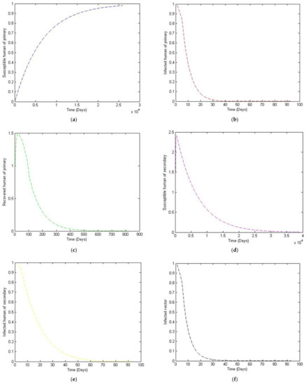
Figure 3. The trajectory of $S_{HP}, I_{HP}, R_{HP}, S_{HS}, I_{HS}$ and $I_V$ toward the disease-free equilibrium point for $R_0<1$ with parameter values according to Table 1. (a) Susceptibles of primary infection (b) Infected population with primary infection (c) Recovered human of primary infection (d) Susceptibles of secondary infection (e) Infected human of secondary infection (f) Infected vector.

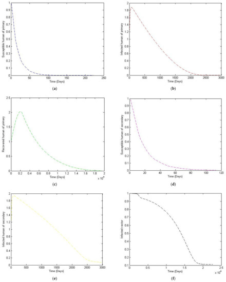
Figure 4. The trajectory of $S_{HP}, I_{HP}, R_{HP}, S_{HS}, I_{HS}$ and $I_V$ toward the endemic equilibrium point, for $R_0>1$ with parameter values according to Table 3. (a) Susceptibles of primary infection (b) Infected population with primary infection (c) Recovered human of primary infection (d) Susceptibles of secondary infection (e) Infected human of secondary infection (f) Infected vector.

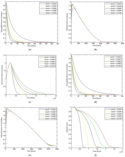
Figure 5. The trajectory of $S_{HP}, I_{HP}, R_{HP}, S_{HS}, I_{HS}$ and $I_V$ toward the endemic equilibrium point for $R_0>1$ with a comparison of the transmission rate of the dengue virus from vector to human, ${\beta }_H=0.0020, 0.0040, 0.0060, 0.0080, 0.0100,$ and parameter values according to Table 3. (a) Susceptibles of primary infection (b) Infected population with primary infection (c) Recovered human of primary infection (d) Susceptibles of secondary infection (e) Infected human of secondary infection (f) Infected vector.

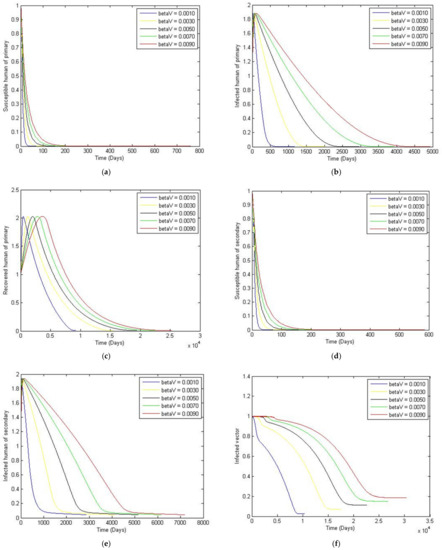
Figure 6. The trajectory of $S_{HP}, I_{HP}, R_{HP}, S_{HS}, I_{HS}$ and $I_V$ toward the endemic equilibrium point for $R_0>1$ with a comparison of the transmission rate of the dengue virus from human to vector, ${\beta }_V=0.0010, 0.0030, 0.0050, 0.0070, 0.0090,$ and parameter values according to Table 3. (a) Susceptibles of primary infection (b) Infected population with primary infection (c) Recovered human of primary infection (d) Susceptibles of secondary infection (e) Infected human of secondary infection (f) Infected vector.

For the case of larger cities such as Chiang Mai or Khon Kaen, etc., we assume that:

• Case 1: the number humans $N_H=\mathrm{500,000}$ and the number of vectors $N_V=\mathrm{100,000}$, while for
• Case 2: the number of humans $N_H=\mathrm{500,000}$ and the number of vectors $N_V=\mathrm{100,000}{e}^{\left(-1/14\right)t}$ to investigate their implications.

Note that Case 2 simulates the situation where the size of the vector population is not constant but is rather a function of time. The exponential power of −1/14 is also used to reflect the natural death rate of the vector population. It can be seen from Figure 7 and Figure 8 that there is a small change in trajectory from Case 1 to Case 2, which is to be expected since the total vector population slowly decays.

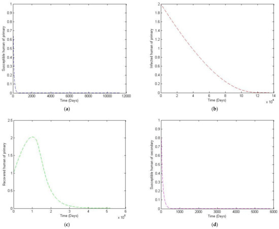
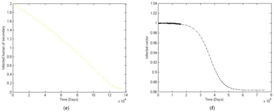
Figure 7. The trajectory of $S_{HP}, I_{HP}, R_{HP}, S_{HS}, I_{HS}$ and $I_V$ toward the endemic equilibrium point for $R_0>1$ with parameter values according to Table 3; changes $N_H=\mathrm{500,000},$ and $N_V=\mathrm{100,000}$. (a) Susceptibles of primary infection (b) Infected population with primary infection (c) Recovered human of primary infection (d) Susceptibles of secondary infection (e) Infected human of secondary infection (f) Infected vector.

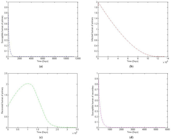
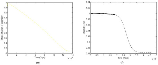
Figure 8. The trajectory of $S_{HP}, I_{HP}, R_{HP}, S_{HS}, I_{HS}$ and $I_V$ toward the endemic equilibrium point for $R_0>1$ with parameter values according to Table 3; changes $N_H=\mathrm{500,000},$ and $N_V=\mathrm{100,000}{e}^{\left(-1/14\right)t}$. (a) Susceptibles of primary infection (b) Infected population with primary infection (c) Recovered human of primary infection (d) Susceptibles of secondary infection (e) Infected human of secondary infection (f) Infected vector.

Sensitivity Analysis of Parameters

The index tells us which parameters have a high impact on the basic reproductive number, $R_0,$ and should be targeted by intervention strategies. In addition, the sensitivity index allows us to measure relative changes in variables as parameters change. The normalized forward sensitivity index of a variable related to a parameter is the ratio of the relative change in the variable to the relative change in the parameter [34].

Definition 4

(Chitnis, Hyman, and Cushing [34]). The normalized forward sensitivity index of $R_0$, which depends differentiably on a parameter $p$, is defined by:

$${\Upsilon }_p^{R_0}=\frac{\partial R_0}{\partial p}\times \frac{p}{R_0}$$

(29)

Given an expression for $R_0$ in Equation (27), the sensitivity index of Equation (29) can now be used to evaluate the index of each parameter. Note that the sensitivity index could be a function of some parameters, or a number, signifying its independence of any parameter. Table 4 shows the sensitivity index of $R_0$ to all the parameters of Table 3.

Table 4. Sensitivity indices ${\Upsilon }_p^{R_0}$ evaluated at the baseline parameter values of Table 1.

Parameters	Sensitivity
$\alpha$	0.5
$N_H$	0.5
$N_V$	0.5
${\beta }_H$	0.5
${\beta }_V$	0.5
$b$	−0.0001141
$d_V$	−0.1666667
$d_d$	−0.20825858
$d_k$	−0.3333333
${\gamma }_P$	−0.2916001

Figure 9 plots a comparison of the $R_0$ values against the changes in $d_d$ and ${\gamma }_P$. It can be seen that as the $d_d$ and ${\gamma }_P$ values change, the increment of $R_0$ in $d_d$ is more pronounced than that of ${\gamma }_P$. This is reflected in the ${\Upsilon }_p^{R_0}$ index, where ${\Upsilon }_{d_d}^{R_0}$ is significantly larger than ${\Upsilon }_{{\gamma }_P}^{R_0}$. Note that a similar definition to Equation (29) with regards to the sensitivity of $I_V^{*}$ with respect to the parameters could also be given. However, due to the algebraic complexities of $I_V^{*}$ in Equation (26), a numerical plot is instead given. It is apparent in Figure 10 that as ${\beta }_V$ changes, the endemic equilibrium $I_V^{* }$ also changes somewhat linearly.

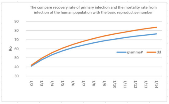
Figure 9. A comparison of parameters between $d_d$ and ${\gamma }_P$ with $R_0$.

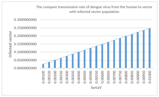
Figure 10. A comparison of parameters between ${\beta }_V$ with $I_V{}^{*}$.

4. The Optimal Control Problem

In this section, the solution of the optimal control problem is discussed. The Pontryagin Minimum Principle (PMP) theory is used to solve this problem. Equations (19)–(24) will be recast as a control problem. The purpose of this is to recast the problem as one of minimizing the number of infected humans to achieve an optimal outcome. Since, the system consists of two dynamics, one for the humans and the other for the vectors, two control parameters will be needed, $u_1$ for the human population and $u_2$ for the vector population. $u_1$ is the vaccination rate and $u_2$ is the rate at which the breeding of the Aegypti mosquitoes is annihilated. This model can be written as the system of the equation as follows:

$$\frac{d{S}_{HP}}{dt}=b-\alpha {\beta }_H{S}_{HP}{I}_V{N}_V-b{S}_{HP}$$

(30)

$$\frac{d{I}_{HP}}{dt}=\alpha {\beta }_H{S}_{HP}{I}_V{N}_V-{\gamma }_P{I}_{HP}-\left(b+d_d\right)I_{HP}$$

(31)

$$\frac{d{R}_{HP}}{dt}={\gamma }_P{I}_{HP}-\left(1-\psi \right)\theta R_{HP}-b{R}_{HP}$$

(32)

$$\frac{d{S}_{HS}}{dt}=\left(1-\psi \right)\theta R_{HP}-\alpha {\beta }_H{S}_{HS}{I}_V{N}_V-b{S}_{HS}-u_1\left(t\right)I_{HS}$$

(33)

$$\frac{d{I}_{HS}}{dt}=\alpha {\beta }_H{S}_{HS}{I}_V{N}_V-{\gamma }_S{I}_{HS}-b{I}_{HS}$$

(34)

$$\frac{d{R}_{HS}}{dt}={\gamma }_S{I}_{HS}-b{R}_{HS}$$

(35)

$$\frac{d{S}_V}{dt}=\frac{A}{N_V}-{\beta }_V{S}_V\left(I_{HP}+I_{HS}\right)N_H-d_V{S}_V-u_2\left(t\right)S_V$$

(36)

$$\frac{d{I}_V}{dt}={\beta }_V{S}_V\left(I_{HP}+I_{HS}\right)N_H-\left(d_V+d_k\right)I_V-u_2\left(t\right){\beta }_V{S}_V\left(I_{HP}+I_{HS}\right)N_H$$

(37)

In terms of the normalized compartments, the differential equations become:

$$\frac{d{S}_{HP}}{dt}=b-\alpha {\beta }_H{S}_{HP}{I}_V{N}_V-b{S}_{HP}$$

(38)

$$\frac{d{I}_{HP}}{dt}=\alpha {\beta }_H{S}_{HP}{I}_V{N}_V-{\gamma }_P{I}_{HP}-\left(b+d_d\right)I_{HP}$$

(39)

$$\frac{d{R}_{HP}}{dt}={\gamma }_P{I}_{HP}-\left(1-\psi \right)\theta R_{HP}-b{R}_{HP}$$

(40)

$$\frac{d{S}_{HS}}{dt}=\left(1-\psi \right)\theta R_{HP}-\alpha {\beta }_H{S}_{HS}{I}_V{N}_V-b{S}_{HS}-u_1\left(t\right)I_{HS}$$

(41)

$$\frac{d{I}_{HS}}{dt}=\alpha {\beta }_H{S}_{HS}{I}_V{N}_V-{\gamma }_S{I}_{HS}-b{I}_{HS}$$

(42)

$$\frac{d{I}_V}{dt}={\beta }_V{S}_V\left(I_{HP}+I_{HS}\right)N_H-\left(d_V+d_k\right)I_V-u_2\left(t\right){\beta }_V{S}_V\left(I_{HP}+I_{HS}\right)N_H$$

(43)

All parameters retain same definitions as before. The optimal control problems of Equations (38)–(43), require a definition of the objective function given as:

$$J\left(u_1,u_2\right)=\min \underset{0}{\overset{T}{{\displaystyle \int }}}\left[X_1{I}_{HP}+X_2{I}_{HS}+\frac{1}{2}\left(X_3{u}_1^2\left(t\right)+X_4{u}_2^2\left(t\right)\right)\right]dt$$

(44)

with initial condition $S_{HP}\ge 0, I_{HP}\ge 0, R_{HP}\ge 0, S_{HS}\ge 0, I_{HS}\ge 0, R_{HS}\ge 0,S_V\ge 0,$ and $I_V\ge 0$. The constants $X_1, X_2, X_3,$ and $X_4$ are weight constants and the terms $X_3{u}_1^2\left(t\right)$ and $X_4{u}_2^2\left(t\right)$ represent the costs associated with the control variables $u_1$ and $u_2,$ respectively. We can assign an optimal solution of this model optimal control problem by using the Lagrangian and the Hamiltonian of the problems. The Lagrangian of the optimal control problem is given by:

$$L\left(I_H,I_V,u_1,u_2\right)=X_1{I}_{HP}+X_2{I}_{HS}+\frac{1}{2}\left(X_3{u}_1^2\left(t\right)+X_4{u}_2^2\left(t\right)\right)$$

(45)

Theorem 3.

We consider the objective function$J$given by Equation (44) with$\left(u_1,u_2\right)\in U$subjecting to the control system of Equations (38)–(43) with initial condition. There exists$u^{*}\left(t\right)=\left\{u_1^{*}\left(t\right),u_2^{*}\left(t\right)\right\}\in U$such that$J\left(u_1^{*},u_2^{*}\right)=min\left\{J\left(u_1,u_2\right)\left|\left(u_1,u_2\right)\in U\right.\right\}$.

Proof. 

See the proof of Theorem A3 in Appendix A. □

Theorem 4.

There exists the adjoint variables${\lambda }_1, {\lambda }_2, {\lambda }_3,{\lambda }_4, {\lambda }_5,$and${\lambda }_6$under the control that satisfies the following:

$$\begin{gathered} \frac{d{\lambda }_1}{dt}={\lambda }_1\left(t\right)\left(\alpha {\beta }_H{I}_V{N}_V+b\right)-{\lambda }_2\left(t\right)\left(\alpha {\beta }_H{I}_V{N}_V\right), \\ \frac{d{\lambda }_2}{dt}=-X_1+{\lambda }_2\left(t\right)\left({\gamma }_P+d_d+b\right)-{\lambda }_3\left(t\right){\gamma }_P-{\lambda }_6\left(t\right)\left({\beta }_V{N}_H\left(1-I_V-u_2^{*}\left(t\right)+I_V{u}_2^{*}\left(t\right)\right)\right), \\ \frac{d{\lambda }_3}{dt}={\lambda }_3\left(t\right)\left(\left(1-\psi \right)\theta +b\right)-{\lambda }_4\left(t\right)\left(\left(1-\psi \right)\theta \right), \\ \frac{d{\lambda }_4}{dt}={\lambda }_4\left(t\right)\left(\alpha {\beta }_H{I}_V{N}_V+b\right)-{\lambda }_5\left(t\right)\left(\alpha {\beta }_H{I}_V{N}_V\right), \\ \frac{d{\lambda }_5}{dt}=-X_2+{\lambda }_4\left(t\right)\left(u_1^{*}\left(t\right)\right)+{\lambda }_5\left(t\right)\left({\gamma }_S+b\right)-{\lambda }_6\left(t\right)\left({\beta }_V{N}_H\left(1-I_V-u_2^{*}\left(t\right)+I_V{u}_2^{*}\left(t\right)\right)\right), \\ \begin{array}{c}\frac{d{\lambda }_6}{dt}={\lambda }_1\left(t\right)\left(\alpha {\beta }_H{S}_{HP}{N}_V\right)-{\lambda }_2\left(t\right)\left(\alpha {\beta }_H{S}_{HP}{N}_V\right)+{\lambda }_4\left(t\right)\left(\alpha {\beta }_H{S}_{HS}{N}_V\right)\\ -{\lambda }_5\left(t\right)\left(\alpha {\beta }_H{S}_{HS}{N}_V\right)+{\lambda }_6\left(t\right)\left({\beta }_V{N}_H\left(1-u_2^{*}\left(t\right)\right)\left(I_{HP}+I_{HS}\right)+\left(d_V+d_k\right)\right).\end{array} \end{gathered}$$

(46)

with the boundary conditions:

$${\lambda }_1\left(t\right)={\lambda }_2\left(t\right)={\lambda }_3\left(t\right)={\lambda }_4\left(t\right)={\lambda }_5\left(t\right)={\lambda }_6\left(t\right)=0$$

(47)

In addition, the optimal control variables are given by:

$$u_1^{*}\left(t\right)=\max \left(\min \left(\frac{{\lambda }_4{I}_{HS}^{*}}{X_3},u_1^{\max }\right),0\right)$$

(48)

$$u_2^{*}\left(t\right)=\max \left(\min \left(\frac{{\lambda }_6\left(1-I_V^{*}\right){\beta }_V\left(I_{HP}^{*}+I_{HS}^{*}\right)N_H}{X_4},u_2^{\max }\right),0\right)$$

(49)

Proof. 

See the proof of Theorem A4 in Appendix A. □

The simulation results for the optimal states are presented in Figure 11, Figure 12, Figure 13, Figure 14 and Figure 15 and the optimal controls are shown in Figure 14 using parameter values according to Table 1.

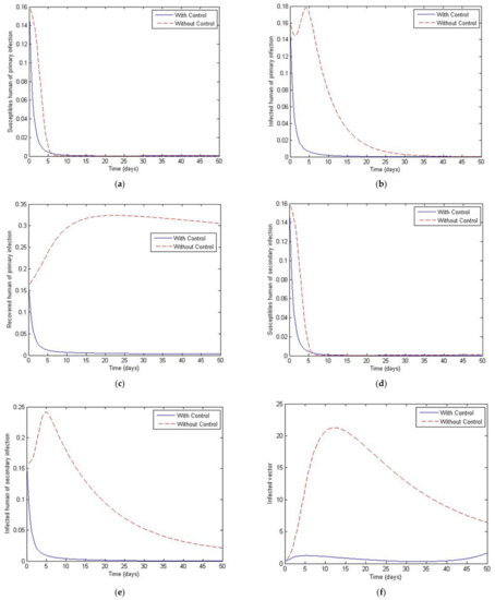
Figure 11. Simulation results of system of Equations (38)–(43) with and without controls of $S_{HP}, I_{HP}, R_{HP}, S_{HS}, I_{HS}$ and $I_V$ for $X_1=100, X_2=100$. (a) Susceptibles of primary infection (b) Infected population with primary infection (c) Recovered human of primary infection (d) Susceptibles of secondary infection (e) Infected human of secondary infection (f) Infected vector.

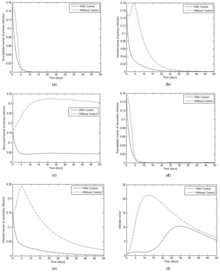
Figure 12. Simulation results of system of Equations (38)–(43) with and without controls of $S_{HP}, I_{HP}, R_{HP}, S_{HS}, I_{HS}$ and $I_V$ with $X_1=50, X_2=100$. (a) Susceptibles of primary infection (b) Infected population with primary infection (c) Recovered human of primary infection (d) Susceptibles of secondary infection (e) Infected human of secondary infection (f) Infected vector.

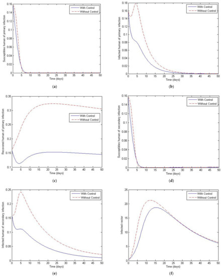
Figure 13. Simulation results of system of Equations (38)–(43) with and without controls of $S_{HP}, I_{HP}, R_{HP}, S_{HS}, I_{HS}$ and $I_V$ when $X_1=0.00001, X_2=100$. (a) Susceptibles of primary infection (b) Infected population with primary infection (c) Recovered human of primary infection (d) Susceptibles of secondary infection (e) Infected human of secondary infection (f) Infected vector.

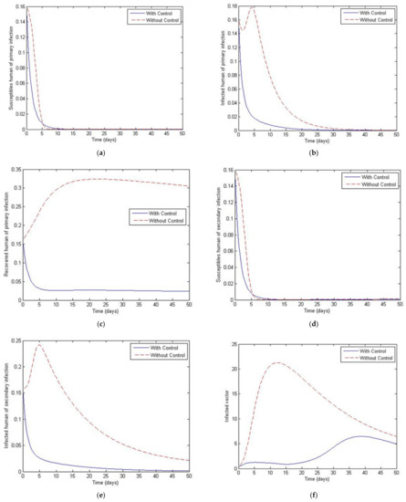
Figure 14. Simulation results of system of Equations (38)–(43) with and without controls of $S_{HP}, I_{HP}, R_{HP}, S_{HS}, I_{HS}$ and $I_V$ when $X_1=100, X_2=50$. (a) Susceptibles of primary infection (b) Infected population with primary infection (c) Recovered human of primary infection (d) Susceptibles of secondary infection (e) Infected human of secondary infection (f) Infected vector.

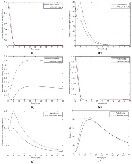
Figure 15. Simulation results of system of Equations (38)–(43) with and without controls of $S_{HP}, I_{HP}, R_{HP}, S_{HS}, I_{HS}$ and $I_V$ when $X_1=100, X_2=0.00001$. (a) Susceptibles of primary infection (b) Infected population with primary infection (c) Recovered human of primary infection (d) Susceptibles of secondary infection (e) Infected human of secondary infection (f) Infected vector.

Figure 11, Figure 12, Figure 13, Figure 14 and Figure 15 show the simulation results of the system of Equations (38)–(43) with and without controls of $S_{HP},I_{HP},R_{HP},S_{HS},I_{HS},$ and $I_V$. The plot of Figure 11 is obtained by setting the weight $X_1$ to be equal to $X_2$. Figure 12 presents the case in which the weight $X_1$ less than $X_2$. Figure 13 presents the case where $X_1$ is at least 10 times greater than $X_2$. Figure 14 presents the case in which the weight $X_1$ is greater than $X_2$. Figure 15 presents the case where $X_1$ is at least 10 times greater than $X_2$. Note that the main goal of the control is to minimize the number of infected humans with primary infection $I_{HP}$, as well as the secondary infection $I_{HS}$. The main emphasis, however, is on the secondary infectious individuals. For each of these scenarios, a comparison is also made with the case where no control is applied. If $X_1=X_2$, the convergence time to equilibrium is significantly faster than if $X_1$ is less than $X_2, X_1$ is much less than $X_2, X_1$ is greater than $X_2,$ and $X_1$ much greater than $X_2$. Moreover, as the weight of $X_1$ increases, the steady state of infected individuals of the secondary population $I_{HS }^{*}$ gradually decreases to zero. The trajectory of the infected vectors gradually deviates from the no-control case. No significant change seems to occur to the trajectories as the weight $X_2$ is increased, except for the infected vectors, which appear to approach zero for a large weight of 100. With no control measures, it will take longer for equilibrium to be reached.

Figure 16a shows that to maintain the optimal control of the infected population, $u_1\left(t\right)$ would have to be at 50%, 70%, and 90% for the first 25 days, after which the control required will show an exponential decline to zero. Figure 16b shows the values required to maintain optimal control when $u_2\left(t\right)$ is used as the controlling factor. The application of 50%, 70%, and 90% of $u_2\left(t\right)$ for achieving optimal control should be maintained for the first 47 days, after which the amount of control steadily decreases to zero.

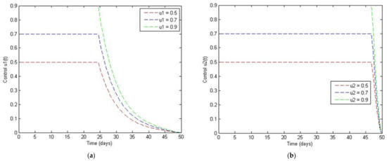
Figure 16. Simulation results of the control: (a) The vaccination rate $u_1\left(t\right)$ and (b) the Aegypti breeding destroying rate $u_2\left(t\right)$ when $X_1=100, X_2=100$.

Figure 17 and Figure 18 plot the cases of $N_H=\mathrm{500,000}$ and $N_V=\mathrm{100,000},$ and of $N_H=\mathrm{500,000}$ and $N_V=\mathrm{100,000}{e}^{\left(-1/14\right)t}, \mathrm{respectively}.$ The later values were chosen to investigate the case where the total vector population is not constant. Both figures show a significant decay of both the primary and secondary infective populations to zero in the controlled population compared to the uncontrolled population, which peaks at around 0.25 before decaying to about zero. Note that there is again a small change across the trajectories from Figure 17 to Figure 18, which is to be expected since the total number of vectors is slowly decayed as a function of time.

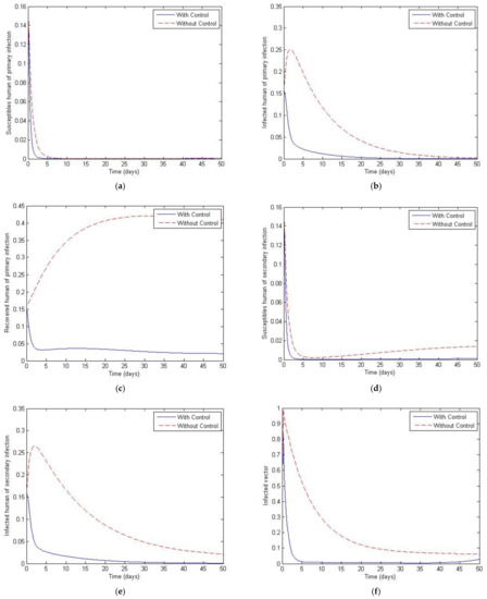
Figure 17. Simulation results of system of Equations (38)–(43) with and without controls of $S_{HP}, I_{HP}, R_{HP}, S_{HS}, I_{HS}$ and $I_V$ with $X_1=100, X_2=100, N_H=\mathrm{500,000}, N_V=\mathrm{100,000}$. (a) Susceptibles of primary infection (b) Infected population with primary infection (c) Recovered human of primary infection (d) Susceptibles of secondary infection (e) Infected human of secondary infection (f) Infected vector.

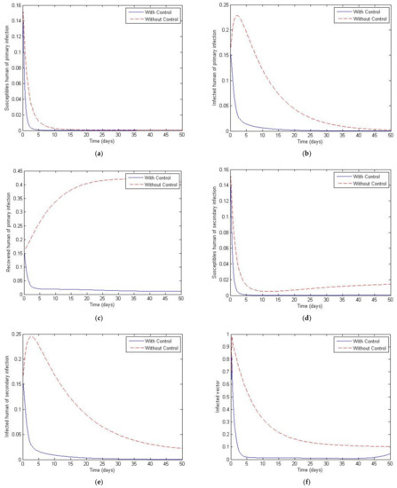
Figure 18. Simulation results of system of Equations (38)–(43) with and without controls of $S_{HP}, I_{HP}, R_{HP}, S_{HS}, I_{HS}$ and $I_V$ with $X_1=100, X_2=100, N_H=\mathrm{500,000}, N_V=\mathrm{100,000}{e}^{\left(-1/14\right)t}$. (a) Susceptibles of primary infection (b) Infected population with primary infection (c) Recovered human of primary infection (d) Susceptibles of secondary infection (e) Infected human of secondary infection (f) Infected vector.

5. Discussion and Conclusions

In this paper, we analyzed the effects of different vaccination strategies to prevent secondary dengue infection in order to reduce the severity of the disease. The dynamic of the dengue fever transmission model assumes that the human and vector population are constant. The analysis was based on the use of the Routh–Hurwitz criteria to establish local asymptotic stability. The equilibrium points that we found were disease-free convergence to $E_1=\left(1,0,0,0,0,0\right)$ and the endemic equilibrium point. The basic reproductive number was defined as $R_0$. If $R_0$ is less than one, then the disease-free state exits and is locally asymptotically stable; it is unstable when $R_0$ is greater than one. We simulated the numerical solution of the parameters with different values, as shown in Figure 5. We can see that if the transmission rate of dengue virus from vector to human ${\beta }_H$ is large, then the convergence to an equilibrium point becomes slower for susceptible humans to primary and secondary infection. The number of humans recovered from primary infection, the number of humans with primary or secondary infection, and the number of infected vectors will converge to an equilibrium point more rapidly. Likewise, in Figure 6, we see that if the transmission rate of the dengue virus from human to vector ${\beta }_V$ is large, then there is a slower convergence to an equilibrium point of the susceptible humans. Similarly, humans who recovered from a primary infection, humans infected with a primary or secondary infection, and infected humans will converge to an equilibrium point more quickly, i.e., $E_2\left(S_{HP}=0.00003,I_{HP}=0.00022,R_{HP}=0.00810,S_{HS}=0.00002,I_{HS}=0.00031\right).$ However, the infected vector will converge to a different equilibrium point. In addition, this will also make the basic reproductive number $R_0$ greater than one. Changing ${\beta }_V$ to a different value affects the convergence time for reaching the equilibrium point, as shown in Figure 8. To investigate whether there is a limitation on the model when there is a non-constant total vector population $N_V$, two further cases were also considered. The first case had the largest total human population $N_H$ at 500,000, and a large $N_V$ of 100,000. The second case kept $N_H$ the same, whilst the $N_V$ was treated as an exponential function of time. Results showed that although having a non-constant $N_V$ does have some effect on the trajectories, such a change is quite small compared to that of the constant vector population case.

We adopted an optimal control approach using the vaccination rate and a rate for destroying the breeding of the Aegypti mosquito in order to minimize the number of humans with primary or secondary infections. To do this, we used the Pontryagin Minimum Principle (PMP) method to solve the optimal control problem with conditions $X_1$ equal $X_2, X_1$ less than $X_2, X_1$ much less than $X_2, X_1$ greater than $X_2,$ and $X_1$ much greater than $X_2.$ We can see that, if there are no controls, the number of humans with primary or secondary infections increases. This will cause the solution to converge to the equilibrium point over a longer time. With the controls in place, the number of mosquitoes in the infected vector population and the number of people who need to be vaccinated will decrease over time, as shown in Figure 11, Figure 12, Figure 13, Figure 14, Figure 15, Figure 16, Figure 17 and Figure 18.

References

- World Health Organization. Dengue and Severe Dengue. Available online: https://www.who.int/news-room/fact-sheets/detail/dengue-and-severe-dengue (accessed on 5 January 2021).
- Aguas, R.; Dorigatti, I.; Coudeville, L.; Luxembrurger, C.; Ferguson, N.M. Cross-serotype interactions and disease outcome prediction of dengue infections in Vietnam. Sci. Rep. 2019, 9, 1–12. [Google Scholar] [CrossRef]
- Guzman, M.G.; Harris, E. Dengue. Lancet 2015, 385, 453–465. [Google Scholar] [CrossRef]
- Esteva, L.; Vargas, C. Coexistence of different serotypes of dengue virus. J. Math. Biol. 2003, 46, 31–47. [Google Scholar] [CrossRef] [PubMed]
- Gubler, D.J. Dengue and dengue hemorrhagic fever. Clin. Microbiol. Rev. 1998, 11, 480–496. [Google Scholar] [CrossRef]
- Chaturvedi, U.C.; Nagar, R. Dengue and dengue haemorrhagic fever: Indian perspective. J. Biosci. 2008, 33, 429–441. [Google Scholar] [CrossRef]
- Adams, B.; Holmes, E.C.; Zhang, C.; Mammen, M.P., Jr.; Nimmannitya, S.; Kalayanarooj, S.; Boots, M. Cross-protective immunity can account for the alternating epidemic pattern of dengue virus serotypes circulating in Bangkok. Proc. Natl. Acad. Sci. USA 2006, 103, 14234–14239. [Google Scholar] [CrossRef] [PubMed]
- Capeding, M.R.; Tran, N.H.; Hadinegoro, S.R.S.; Ismail, H.I.H.M.; Chotpitayasunondh, T.; Chua, M.N.; Luong, C.Q.; Rusmil, K.; Wirawan, D.N.; Nallusamy, R.; et al. Clinical efficacy and safety of a novel tetravalent dengue vaccine in healthy children in Asia: A phase 3, randomised, observer-masked, placebo-controlled trial. Lancet 2014, 384, 1358–1365. [Google Scholar] [CrossRef]
- World Health Organization. Fact Sheet: Questions and Answers on Dengue Vaccines: Phase III Study of CYD-TDV. Available online: http://www.who.int/immunization/research/development/WHO_dengue_vaccine_QA_July2014.pdf (accessed on 5 January 2021).
- Villar, L.; Dayan, G.H.; Arredondo-Garcia, J.L.; Rivera, D.M.; Cunha, R.; Deseda, C.; Reynales, H.; Costa, M.S.; Morales-Ramirez, J.O.; Carrasquilla, G.; et al. Efficacy of a tetravalent dengue vaccine in children in Latin America. N. Engl. J. Med. 2015, 372, 113–123. [Google Scholar] [CrossRef]
- Biswal, S.; Reynales, H.; Saez-Llorens, X.; Lopez, P.; Borja-Tabora, C.; Kosalaraksa, P.; Sirivichayakul, C.; Watanaveeradej, V.; Rivera, L.; Espinoza, F.; et al. Efficacy of a tetravalent dengue vaccine in healthy children and adolescents. N. Engl. J. Med. 2019, 381, 2009–2019. [Google Scholar] [CrossRef]
- Sabchareon, A.; Wallace, D.; Sirivichayakul, C.; Limkittikul, K.; Chanthavanich, P.; Suvannadabba, S.; Jiwariyavej, V.; Dulyachai, W.; Pengsaa, K.; Wartel, T.A.; et al. Protective efficacy of the recombinant, live-attenuated, CYD tetravalent dengue vaccine in Thai schoolchildren: A randomised, controlled phase 2b trial. Lancet 2012, 380, 1559–1567. [Google Scholar] [CrossRef]
- World Health Organization. Updated Questions and Answers Related to the Dengue Vaccine Dengvaxia® and Its Use. Available online: https://www.who.int/immunization/diseases/dengue/q_and_a_dengue_vaccine_dengvaxia_use/en/ (accessed on 5 January 2021).
- Esteva, L.; Vargas, C. A model for dengue disease with variable human population. J. Math. Biol. 1999, 38, 220–240. [Google Scholar] [CrossRef]
- Pongsumpun, P.; Kongnuy, R.; Lopez, D.G.; Tang, I.M.; Dubois, M.A. Contact infection spread in an SEIR model: An analytical approach. Sci. Asia 2013, 39, 410–415. [Google Scholar] [CrossRef][Green Version]
- Pongsumpun, P. The dynamical model of dengue vertical transmission. Curr. Appl. Sci. Technol. 2017, 17, 48–61. [Google Scholar]
- Chanprasopchai, P.; Tang, I.M.; Pongsumpun, P. The SEIR dynamical transmission model of dengue disease with and without the vertical transmission of the virus. Am. J. Appl. Sci. 2017, 14, 1123–1145. [Google Scholar] [CrossRef][Green Version]
- Syafruddin, S.; Noorani, S.M. A SIR model for spread of dengue fever disease (simulation for south sulawesi Indonesia and selangor Malaysia). World J. Model. Simul. 2013, 9, 96–105. [Google Scholar]
- Yaacob, Y. Analysis of a dengue disease transmission model without immunity. MATEMATIKA Malays. J. Ind. Appl. Math. 2007, 23, 75–81. [Google Scholar]
- Singh, B.; Jain, S.; Khandelwal, R.; Porwal, S.; Ujjainkar, G. Analysis of a dengue disease transmission model with vaccination. Adv. Appl. Sci. Res. 2014, 5, 237–242. [Google Scholar]
- Tasman, H.; Supriatna, A.K.; Nuraini, N.; Soewono, E. A dengue vaccination model for immigrants in a two-age-class population. Int. J. Math. Math. Sci. 2012, 2012, 236352. [Google Scholar] [CrossRef]
- Aguiar, M.; Stollenwerk, N.; Halstead, S.B. The impact of the newly licensed dengue vaccine in endemic countries. PLoS Negl Trop Dis. 2016, 10, e0005179. [Google Scholar] [CrossRef] [PubMed]
- Aguiar, M.; Stollenwerk, N. Mathematical models of dengue fever epidemiology: Multi-strain dynamics, immunological aspects associated to disease severity and vaccines. Commun. Biomath. Sci. 2017, 1, 1–12. [Google Scholar] [CrossRef]
- Viriyapong, R.; Tavaen, S. Global stability and optimal control of melioidosis transmission model with hygiene care and treatment. NU. Int. J. Sci. 2019, 16, 31–48. [Google Scholar]
- Rodrigues, H.S.; Monteiro, M.T.T.; Torres, D.F.M. Dynamics of dengue epidemics when using optimal control. Math. Comput. Model. 2010, 52, 1667–1673. [Google Scholar] [CrossRef]
- Rodrigues, H.S.; Monteiro, M.T.T.; Torres, D.F.M. Vaccination models and optimal control strategies to dengue. Math. Biosci. 2014, 247, 1–12. [Google Scholar] [CrossRef] [PubMed]
- Agustoa, A.B.; Khan, M.A. Optimal control strategies for dengue transmission in Pakistan. Math. Biosci. 2018, 305, 102–121. [Google Scholar] [CrossRef]
- Ndii, M.Z.; Mage, A.R.; Messakh, J.J.; Djahi, B.S. Optimal vaccination strategy for dengue transmission in Kupang city, Indonesia. Heliyon 2020, 6, e05345. [Google Scholar] [CrossRef] [PubMed]
- Ministry of Public Health Thailand. Dengue Fever. Available online: http://www.boe.moph.go.th/boedb/surdata/disease.php?dcontent=old&ds=66 (accessed on 5 January 2021).
- Diekmann, O.; Heesterbeek, J.A.P.; Roberts, M.G. The construction of next-generation matrices for compartmental epidemic models. J. R. Soc. Interface 2010, 7, 873–885. [Google Scholar] [CrossRef]
- Wu, C.Q.; Wong, P.J.Y. Dengue transmission: Mathematical model with discrete time delays and estimation of the reproduction number. J. Biol. Dyn. 2019, 13, 1–25. [Google Scholar] [CrossRef] [PubMed]
- Prathumwan, D.; Trachoo, K.; Chaiya, I. Mathematical modeling for prediction dynamics of the coronavirus disease 2019 (COVID-19) pandemic, quarantine control measures. Symmetry 2020, 12, 1404. [Google Scholar] [CrossRef]
- NewsDesk. Thailand Reports 71,000 Dengue Cases in 2020. Available online: outbreaknewstoday.com/thailand-reports-71000-dengue-cases-in-2020/ (accessed on 16 July 2021).
- Chitnis, N.; Hyman, J.M.; Cushing, J.M. Determining important parameters in the spread of malaria through the sensitivity analysis of a mathematical model. Bull. Math. Biol. 2008, 70, 1272–1296. [Google Scholar] [CrossRef]
- Lukes, D.L. Differential Equations: Classical to Controlled; Academic Press: London, UK; New York, NY, USA, 1982. [Google Scholar]
- Chanprasopchai, P.; Tang, I.M.; Pongsumpun, P. SIR model for dengue disease with effect of dengue vaccination. Comput. Math. Methods Med. 2018, 2018, 9861572. [Google Scholar] [CrossRef]
- Xue, L.; Ren, X.; Magpantay, F.; Sun, W.; Zhu, H. Optimal control of mitigation strategies for dengue virus transmission. Bull. Math. Biol. 2021, 83, 1–28. [Google Scholar] [CrossRef] [PubMed]
- Lenhart, S.; Workman, J.T. Optimal Control Applied to Biological Models; Chapman and Hall/CRC: Boca Raton, FL, USA; New York, NY, USA, 2007. [Google Scholar]
Publisher’s Note: MDPI stays neutral with regard to jurisdictional claims in published maps and institutional affiliations. |
© 2021 by the authors. Licensee MDPI, Basel, Switzerland. This article is an open access article distributed under the terms and conditions of the Creative Commons Attribution (CC BY) license (https://creativecommons.org/licenses/by/4.0/).