Numerical Investigation of Fuzzy Predator-Prey Model with a Functional Response of the Form Arctan(ax)

Abstract

In this paper we study a fuzzy predator-prey model with functional response $arctan\left(ax\right).$ The fuzzy derivatives are approximated using the generalized Hukuhara derivative. To execute the numerical simulation, we use the fuzzy Runge-Kutta method. The results obtained over time for the evolution and the population are presented numerically and graphically with some conclusions.

1. Introduction

The concept of fuzzy valued functions was studied by many authors, see [1,2,3,4,5,6,7]. In general, they based their definition of derivatives on the concept of Hukuhara derivative for set valued functions. Bede and Gal [1] introduced strongly generalized derivatives since with time the Hukuhara derivative fuzzifies the solution.

In applied sciences and engineering, differential equations are commonly used to represent real life problems and systems. In many practical cases uncertainties can appear. This gives rise to fuzzy differential equations and many authors defined fuzzy differential equations with a derivative based on Hukuhara derivative and its generalizations, see [1,2,4,8,9]. In addition, several numerical methods were developed to solve fuzzy initial and boundary value problems, see [10,11,12,13,14,15].

Assume that the initial value problem has an uncertain initial value modeled by a fuzzy interval, then the fuzzy initial value problem will be

$$X^{\prime }\left(t\right)=f\left(t,X\left(t\right)\right),X\left(t_0\right)=X_0$$

where $f:[0,T]\times R_F^n\to R_F^n$ is a fuzzy interval-valued function and $X_0\in R_F^n$, the set of fuzzy numbers, have been developed to solve fuzzy differential equations, [16].

Our concern is to consider the predator-prey model that has the form

$$\begin{array}{ccc}\hfill \frac{dX}{dt}& =& aX-bXY\hfill \\ \hfill \frac{dY}{dt}& =& -cY+dXY,\hfill \end{array}$$

(1)

where $a,b,c$ and d are positive constants, a is the growth rate of the prey, c is the death rate of the predator, and b and d are measures of the effect of the interaction between the predator and the prey.

Many authors studied the predator-prey models with uncertainty in the initial populations of the predator and the prey. They gave numerical solutions to differential equations with fuzzy initial conditions and some discussed the stability of the solutions [10,11,17,18,19].

For example, Ahmed and Baets [10] studied a predator-prey population model with fuzzy initial populations of predator and prey. They did some simulations to the model numerically by means of a 4th-order Runge-Kutta method. They obtained fuzzy stable equilibrium points. Euler method was used by Ahmed and Hasan [11] and Akin and Oruc [17] used the concept of generalized differentiability to solve the Lotka–Voltera model.

Stability of the model was studied by [18,19]. In [19], the authors did simulation of the interaction between aphids (preys) and ladybugs (predators) in addition to studying the stability of the critical points. Existence of limit cycles was done for a model with functional response in [20]. Numerical computations were done in [21] to compare the fuzzy solution with the deterministic one. In [22], the authors concluded the superiority of the fuzzy solution over the crisp one. Numerical simulation to derive conditions of Turing and Hopf bifurcation around the steady state solution was done by [23].

Predator prey model with harvesting was considered by [24,25,26,27,28] where in [25], the authors studied the stability and the bionomic analysis in the presence of toxicity. While in [24], the authors considered a fractional predator prey model numerically in addition to studying the stability, existence, and uniqueness of the solution. In [26], the authors considered a model that incorporates the effects of prey refuge and predator mutual interference. A model with infectious disease in the prey population was considered by [27] where they proved local stability of the system at equilibrium points. The authors in [28] considered a system with two competing species affected by harvesting and the presence of a predator. They presented some numerical examples to support their findings.

In this paper, we follow the footsteps of [20], we consider the predator prey model with functional response $arctan\left(ax\right)$ of the form

$$\begin{array}{ccc}\hfill X^{\prime }\left(t\right)& =& RX\left(1-X\right)-Yarctan\left(aX\right)\hfill \\ \hfill Y^{\prime }\left(t\right)& =& -DY+SYarctan\left(aX\right)\hfill \end{array}$$

(2)

where R, S and D are positive constants and X and Y are the population sizes of the prey and the predator respectively. We convert the model to a fuzzy model with fuzzy initial conditions and study the resulting different cases (to be explained) numerically. We investigate which system has a solution that makes sense and is stable. We then fuzzify the parameters of the model and repeat the study again and present the results numerically and graphically.

The outline of the paper will be as follows. In Section 2, we present the basic concepts and some needed definitions that paves the way to numerical investigation. Section 3 will contain the different types of models with fuzzy initial values and with fuzzy parameters together with the numerical results. The last section will contain some conclusions.

2. Basic Concepts

We start by some needed basic concepts:

Definition 1.

A fuzzy subset A of some set Ω is defined by its membership function, written $A\left(x\right)$, which produces values in $[0,1]$ for all x in$\Omega$. That is; $A\left(x\right)$ is a function mapping Ω into $[0,1]$. If $A\left(x\right)$ is always equal to one or zero then the subset A is said to be crisp (classical) set.

Definition 2.

Let A be a fuzzy subset of Ω. An α – level of$A$, written ${\left[A\right]}_{\alpha }$, is defined as $\{x\in \Omega :A(x)\ge \alpha \}$ for $0<\alpha \le 1$. ${\left[A\right]}_0$, the support of A is defined as the closure of the union of all the ${\left[A\right]}_{\alpha }$, for $0<\alpha \le 1$. The core of A is the set of all elements in Ω with membership degree in A equal to $1.$

Definition 3.

A fuzzy number $N$ is a fuzzy subset of the real numbers satisfying: $\left(i\right)\exists x:N\left(x\right)=1,$ $\left(ii\right)$${\left[N\right]}_{\alpha }$ is a closed and bounded interval for $0\le \alpha \le 1$.

The family of all fuzzy numbers will be denoted by $R_F$.

A special type of fuzzy numbers $M=[a_1,a_2,a_3]$ with $a_1<a_2<a_3$ is called tringular fuzzy number if it satisfies the following, [10]:

$$M\left(x\right)=\left\{\begin{array}{ccc}0\hfill & \mathrm{if}& x\le a_1\mathrm{or}x\ge a_3\hfill \\ 1\hfill & \mathrm{if}& x=a_2\hfill \\ \mathrm{Straight} \mathrm{line}\hfill & \mathrm{if}& x\in \left[a_1,a_2\right] \mathrm{or} x\in \left[a_2,a_3\right]\hfill \end{array}\right.,$$

note that $M\left(x\right)$ is called a triangular shaped fuzzy number if one of the graphs above is a curve and not a straight line and we write$M\approx (a_1,a_2,a_3)$. While the fuzzy number $M=[a_1,a_2,a_3,a_4]$ with $a_1<a_2<a_3<a_4$ is called trapezoidal fuzzy number if it satisfies the following, [10]:

$$M\left(x\right)=\left\{\begin{array}{ccc}0\hfill & \mathrm{if}& x\le a_1\mathrm{or}x\ge a_4\hfill \\ 1\hfill & \mathrm{if}& x=[a_2,a_3]\hfill \\ \mathrm{Straight} \mathrm{line}\hfill & \mathrm{if}& x\in \left[a_1,a_2\right] \mathrm{or} x\in \left[a_3,a_4\right]\hfill \end{array}\right..$$

Again, note that $M\left(x\right)$ is called a trapezoidal shaped fuzzy number if one of the graphs above is a curve and not a straight line and we write $M\approx \left(a_1,a_2,a_3,a_4\right)$.

A fuzzy number is determined by its alpha cuts, $\alpha \in [0,1].$ These alpha cuts satisfy the relation: if ${\alpha }_1>{\alpha }_2$ then ${\left[A\right]}_{{\alpha }_1}\subset {\left[A\right]}_{{\alpha }_2}$, where ${\alpha }_1,{\alpha }_2\in [0,1]$. More details, properties and operations can be found in [2,4,8,29]. Other types of fuzzy numbers and their orders can be found in [12,16,30].

If u is a fuzzy number, then ${\left[u\right]}_{\alpha }=\left[u_{1\alpha },u_{2\alpha }\right]$ where $u_{1\alpha }=min\{s:s\in U\left[\alpha \right]\}$ and $u_{2\alpha }=max\{s:s\in U\left[\alpha \right]\}$ for each $\alpha \in \left[0,1\right].$

Theorem 1

([2,8]). Suppose that $u_1,u_2:[0,1]\to R$ satisfy the following conditions:

- $u_1$ is a bounded increasing function and $u_2$ is a bounded decreasing function with ${\left(u_1\right)}_1\le {\left(u_2\right)}_1$.

- for each $k\in \left(0,1\right],u_1$ and $u_2$ are left-continuous functions at $\alpha =k.$

- $u_1$ and $u_2$are right-continuous at $\alpha =0$.

Then $u:R\to [0,1]$ defined by $u\left(s\right)=sup\{\alpha :u_{1\alpha }\le s\le u_{2\alpha }\}$ is a fuzzy number with parameterization $\left[u_{1\alpha },u_{2\alpha }\right]$. Furthermore, if $u:R\to [0,1]$ is a fuzzy number with parameterization $\left[u_{1\alpha },u_{2\alpha }\right]$, then the functions $u_1$and$u_2$ satisfy the aforementioned conditions.

Definition 4.

The complete metric structure on the set of all fuzzy numbers $R_F$ is given by the Hausdorff distance mapping $D:R_F\times R_F\to [0,\infty )$ such that $D\left(u,v\right)={sup}_{0\le \alpha \le 1}max\{\left|u_{1\alpha }-v_{1\alpha }\right|$, $\left|u_{2\alpha }-v_{2\alpha }\right|\}$ for arbitrary fuzzy numbers $u$and$v.$

Theorem 2

([2,8]). If $u$and$v$ are two fuzzy numbers, then for each $\alpha \in \left[0,1\right],$we have:

$$\begin{array}{ccc}\hfill {\left[u+v\right]}_{\alpha }& =& {\left[u\right]}_{\alpha }+{\left[v\right]}_{\alpha }=\left[u_{1\alpha }+v_{1\alpha },u_{2\alpha }+v_{2\alpha }\right],\hfill \\ \hfill {\left[\mu u\right]}_{\alpha }& =& \mu {\left[u\right]}_{\alpha }=[min\left\{\mu u_{1\alpha },\mu u_{2\alpha }\right\},max\left\{\mu u_{1\alpha },\mu u_{2\alpha }\right\}],\hfill \\ \hfill {\left[uv\right]}_{\alpha }& =& [min\left\{u_{1\alpha }{v}_{1\alpha },u_{1\alpha }{v}_{2\alpha },u_{2\alpha }{v}_{1\alpha },u_{2\alpha }{v}_{2\alpha }\right\},max\left\{u_{1\alpha }{v}_{1\alpha },u_{1\alpha }{v}_{2\alpha },u_{2\alpha }{v}_{1\alpha },u_{2\alpha }{v}_{2\alpha }\right\}].\hfill \end{array}$$

Definition 5.

Let $u,v\in R_F.$ The generalized Hukuhara difference ($gH$-difference) $u{⊝}_{gH}v=w$, where ${w\in R}_F$, if it exists, such that (1) $u=v+w$ or (2) $v=u-w$.

Definition 6.

Let $f:\left[a,b\right]\to R_F.$$f$ is strongly generalized differentiable($GH$-differentiable) at $x_0$ if the limits of some pair of the following exist and are equal:

1. ${\lim }_{h\to 0^{+}}\frac{f(x_0+h)⊝f\left(x_0\right)}{h}$ and ${\lim }_{h\to 0^{+}}\frac{f\left(x_0\right)⊝f(x_0-h)}{h}$.

2. ${\lim }_{h\to 0^{+}}\frac{f\left(x_0\right)⊝f(x_0+h)}{-h}$ and ${\lim }_{h\to 0^{+}}\frac{f(x_0-h)⊝f\left(x_0\right)}{-h}$.

More about Fuzzy calculus can be found in [29].

Definition 7.

Let $f:\left[a,b\right]\to R_F.$f is $1-$differentiable on $\left[a,b\right]$ if f is differentiable in the sense part 1 of the previous definition. Similarly, f is $2-$differentiable on $\left[a,b\right]$ if f is differentiable in the sense part 2 of the previous definition.

Theorem 3.

Let $f:\left[a,b\right]\to R_F$ where ${\left[f\left(x\right)\right]}_{\alpha }=\left[f_{1\alpha }\left(x\right),f_{2\alpha }\left(x\right)\right]$ for each $\alpha \in \left[0,1\right],$

(1) If $f$is $1-$differentiable, then $f_{1\alpha }$and$f_{2\alpha }$ are differentiable functions and ${\left[f^{\prime }\left(x\right)\right]}_{\alpha }=\left[f_{1\alpha }^{\prime }\left(x\right),f_{2\alpha }^{\prime }\left(x\right)\right].$

(2) If $f$is $2-$differentiable, then $f_{1\alpha }$and$f_{2\alpha }$ are differentiable functions and ${\left[f^{\prime }\left(x\right)\right]}_{\alpha }=\left[f_{2\alpha }^{\prime }\left(x\right),f_{1\alpha }^{\prime }\left(x\right)\right].$

3. The Models

In [20], the authors dealt with a general predator prey model of the form

$$\begin{gathered} X^{\prime }\left(t\right)=rX\left(1-X\right)-Y{tan}^{-1}\left(aX\right) \\ {Y}^{\prime }\left(t\right)=-DY+sY{tan}^{-1}\left(aX\right) \end{gathered}$$

(3)

where $X$and$Y$ are the prey and the predator population sizes respectively, $r,s$ and D are positive parameters. Let$\left(X^{*},Y^{*}\right)$be the equilibrium point of (2), then$X^{*}=\frac{1}{a}tan\frac{D}{s}$and$Y^{*}=\frac{rs{X}^{*}(1-X^{*})}{D}$, in addition to $(0,0)$ and $(1,0).$ Where $D,s$and$a$ are chosen such that $0<X^{*}<1$. They established the necessary and sufficient condition for the nonexistence of limit cycles of (2). The system has no limit cycle if and only if

$$tan\left(\frac{D}{s}\right)\left[\frac{stan\left(\frac{D}{s}\right)-2D[1+{tan}^2\left(\frac{D}{s}\right)]}{stan\left(\frac{D}{s}\right)-D[1+{tan}^2\left(\frac{D}{s}\right)]}\right]\ge a.$$

So, if $tan\left(\frac{D}{s}\right)\left[\frac{stan\left(\frac{D}{s}\right)-2D\left[1+{tan}^2\left(\frac{D}{s}\right)\right]}{stan\left(\frac{D}{s}\right)-D\left[1+{tan}^2\left(\frac{D}{s}\right)\right]}\right]<a,$ then there is a limit cycle. Depending on the existence condition we build the following model:

$$\begin{gathered} X^{{}^{\prime }}\left(t\right)=2X\left(1-X\right)-Y{tan}^{-1}\left(5X\right) \\ {Y}^{{}^{\prime }}\left(t\right)=-0.4Y+0.6Y{tan}^{-1}\left(5X\right) \\ {X}_0=1and{Y}_0=1 \end{gathered}$$

(4)

3.1. Fuzzy Initial Conditions

We fuzzify (3) by assuming that$X\left(t\right)$and $Y\left(t\right)$are fuzzy numbers with fuzzy initial conditions. Let ${\left[X\right]}_{\alpha }=\left[u,v\right]$and${\left[Y\right]}_{\alpha }=[r,s]$ and let $x_0=y_0=(0.5,1,1.5)$ be triangular fuzzy numbers, then ${\left[x_0\right]}_{\alpha }={\left[y_0\right]}_{\alpha }=[0.5+\frac{\alpha }{2},1.5-\frac{\alpha }{2}$]. Using the generalized Hukuhara derivatives for $X\left(t\right)$ and $Y\left(t\right)$, consider:

Case 1: Let $X\left(t\right)$and$Y\left(t\right)$be $1-$differentiable then ${[X}^{\prime }{]}_{\alpha }=\left[u^{\prime },v^{\prime }\right]$and${\left[Y^{\prime }\right]}_{\alpha }=\left[r^{\prime },s^{\prime }\right]$. Then the model will be as follows:

$$\begin{array}{ccc}\hfill u^{\prime }& =& 2u-2v^2-s{tan}^{-1}\left(5v\right),\hfill \\ \hfill v^{\prime }& =& 2v-2u^2-r{tan}^{-1}\left(5u\right),\hfill \\ \hfill r^{\prime }& =& -0.4s+0.6r{tan}^{-1}\left(5u\right),\hfill \\ \hfill s^{{}^{\prime }}& =& -0.4r+0.6s{tan}^{-1}\left(5v\right),\hfill \\ \hfill u_0& =& r_0=0.5+\frac{\alpha }{2}and{v}_0=s_0=1.5-\frac{\alpha }{2}.\hfill \end{array}$$

(5)

The equilibrium points of $\left(4\right)$ are ${\chi }_{(0,0)},{\chi }_{(1,0)}$and${\chi }_{(0.157369,0.397811)}$. We solve $\left(4\right)$ using the Fuzzy Runge–Kutta method in Matlab at $\alpha -$levels$=0,0.5,1$. At $\alpha$-level = 0, the solution is given in Table 1 and Figure 1.

Table 1. The solution of $\left(4\right)$ at $\alpha =0$.

Time	$\mathit{u}\left(\mathit{t}\right)$	$\mathit{v}\left(\mathit{t}\right)$	$\mathit{r}\left(\mathit{t}\right)$	$\mathit{s}\left(\mathit{t}\right)$
0.00	0.5000	1.5000	0.5000	1.5000
0.05	0.1826	1.6173	0.4846	1.5563
0.10	−0.2220	1.7863	0.4525	1.6160
0.15	−0.7446	1.9743	0.4049	1.6798
0.20	−1.3939	2.0889	0.3550	1.7480
0.25	−2.1298	2.0063	0.3049	1.8203
0.30	−2.8510	1.5822	0.2552	1.8961
0.35	−3.4498	0.7150	0.2061	1.9726
0.40	−3.8465	−0.6121	0.1580	1.9774
0.45	−4.3524	−2.3905	0.1131	1.8927
0.50	−6.1491	−5.3338	0.0719	1.8069

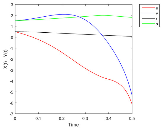
Figure 1. The solution of (4) at $\alpha$ = 0.

At $\alpha$-level = 0.5, the solution is given in Table 2 and Figure 2:

Table 2. The solution of (4) at $\alpha$= 0.5.

Time	$\mathit{u}\left(\mathit{t}\right)$	$\mathit{v}\left(\mathit{t}\right)$	$\mathit{r}\left(\mathit{t}\right)$	$\mathit{s}\left(\mathit{t}\right)$
0.00	0.7500	1.2500	0.7500	1.2500
0.05	0.5664	1.2846	0.7534	1.2888
0.10	0.3465	1.3510	0.7533	1.3295
0.15	0.0756	1.4562	0.7440	1.3724
0.20	−0.2693	1.6206	0.7084	1.4181
0.25	−0.7169	1.8064	0.6560	1.4674
0.30	−1.2786	1.9369	0.6004	1.5205
0.35	−1.9297	1.9132	0.5446	1.5772
0.40	−2.5952	1.6137	0.4895	1.6372
0.45	−3.1783	0.9376	0.4353	1.6989
0.50	−3.6292	−0.1595	0.3822	1.7393
0.55	−3.9949	−1.6588	0.3319	1.6669
0.60	−5.0673	−3.8682	0.2852	1.5879

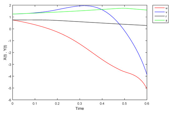
Figure 2. The solution of (4) at $\alpha$ = 0.5.

At $\alpha$-level = 1.0, the solution is Table 3 and Figure 3:

Table 3. The solution of (3) at $\alpha$ = 1.

Time	$\mathit{u}\left(\mathit{t}\right)$	$\mathit{v}\left(\mathit{t}\right)$	$\mathit{r}\left(\mathit{t}\right)$	$\mathit{s}\left(\mathit{t}\right)$
0.0	1.0000	1.0000	1.0000	1.0000
5.0	0.0004	0.0004	0.2800	0.2800
10.0	0.2536	0.2536	0.0598	0.0598
15.0	0.7375	0.7375	0.3892	0.3892
20.0	0.0123	0.0123	0.3867	0.3867
25.0	0.5572	0.5572	0.2186	0.2186
30.0	0.0359	0.0359	0.6595	0.6595
35.0	0.1821	0.1821	0.1628	0.1628
40.0	0.3046	0.3046	0.7312	0.7312
45.0	0.0441	0.0441	0.1979	0.1979
50.0	0.6131	0.6131	0.4784	0.4784
55.0	0.0163	0.0163	0.3125	0.3125
60.0	0.6503	0.6503	0.2871	0.2871
65.0	0.0173	0.0173	0.5135	0.5135
70.0	0.3583	0.3583	0.1827	0.1827
75.0	0.1017	0.1017	0.7595	0.7595
80.0	0.0953	0.0953	0.1683	0.1683
85.0	0.4766	0.4766	0.6195	0.6195
90.0	0.0258	0.0258	0.2402	0.2402
95.0	0.6657	0.6657	0.3817	0.3817
100.0	0.0140	0.0140	0.3900	0.3900

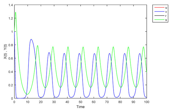
Figure 3. The solution of (4) at $\alpha$ = 1.0.

Case 2:$X\left(t\right)$ is (1)-differentiable$andY\left(t\right)$is (2)-differentiable, then we have the following model:

$$\begin{array}{ccc}\hfill u^{\prime }& =& 2u-2v^2-s{tan}^{-1}\left(5v\right),\hfill \\ \hfill v^{\prime }& =& 2v-2u^2-r{tan}^{-1}\left(5u\right),\hfill \\ \hfill r^{\prime }& =& -0.4r+0.6s{tan}^{-1}\left(5v\right),\hfill \\ \hfill s^{\prime }& =& -0.4s+0.6r{tan}^{-1}\left(5u\right),\hfill \\ \hfill u_0& =& r_0=0.5+\frac{\alpha }{2}\mathrm{and}{v}_0=s_0=1.5-\frac{\alpha }{2}.\hfill \end{array}$$

(6)

Solving (5) at $\alpha -$levels$=0,0.5,1$, the graphs of the solutions are Figure 4, Figure 5 and Figure 6 respectively:

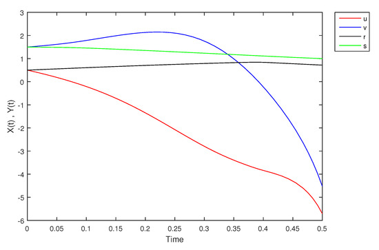
Figure 4. The solution of (5) at $\alpha$ = 0.

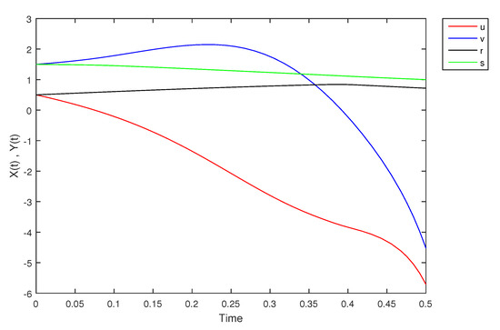
Figure 5. The solution of (5) at $\alpha$ = 0.5.

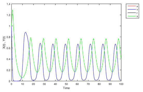
Figure 6. The solution of (5) at $\alpha$ = 1.0.

Case 3:$X\left(t\right)$ is (2)-differentiableand $Y\left(t\right)$is (1)-differentiable, then we have the following model:

$$\begin{array}{ccc}\hfill u^{\prime }& =& 2v-2u^2-r{tan}^{-1}\left(5u\right),\hfill \\ \hfill v^{\prime }& =& 2u-2v^2-s{tan}^{-1}\left(5v\right),\hfill \\ \hfill r^{\prime }& =& -0.4s+0.6r{tan}^{-1}\left(5u\right),\hfill \\ \hfill s^{\prime }& =& -0.4r+0.6s{tan}^{-1}\left(5v\right),\hfill \\ \hfill u_0& =& r_0=0.5+\frac{\alpha }{2}\mathrm{and}{v}_0=s_0=1.5-\frac{\alpha }{2}\hfill \end{array}$$

(7)

Solving (6) at $\alpha -$levels$=0,0.5,1$, the graphs of the solutions are Figure 7, Figure 8 and Figure 9 respectively:

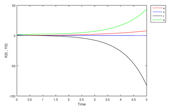
Figure 7. The solution of (6) at $\alpha$ = 0.

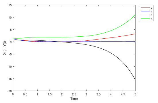
Figure 8. The solution of (6) at $\alpha$ = 0.5.

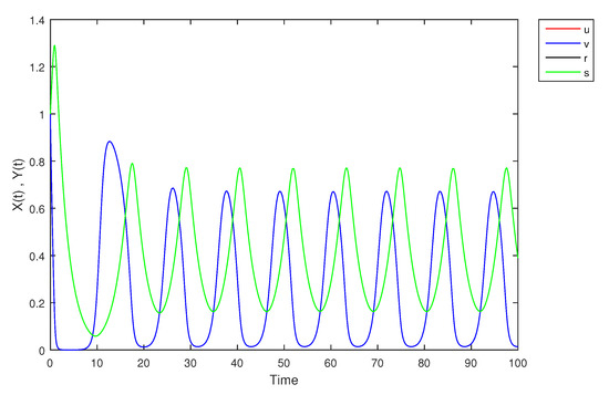
Figure 9. The solution of (6) at $\alpha$ = 1.

Case 4:$X\left(t\right)$and$Y\left(t\right)$are (2)-differentiable, then we have the following model:

$$\begin{array}{ccc}\hfill u^{\prime }& =& 2v-2u^2-r{tan}^{-1}\left(5u\right),\hfill \\ \hfill v^{\prime }& =& 2u-2v^2-s{tan}^{-1}\left(5v\right),\hfill \\ \hfill r^{\prime }& =& -0.4r+0.6s{tan}^{-1}\left(5v\right),\hfill \\ \hfill s^{\prime }& =& -0.4s+0.6r{tan}^{-1}\left(5u\right),\hfill \\ \hfill u_0& =& r_0=0.5+\frac{\alpha }{2}\mathrm{and}{v}_0=s_0=1.5-\frac{\alpha }{2}.\hfill \end{array}$$

(8)

At $\alpha$-level = 0, the solution is shown in Figure 10 and Figure 11.

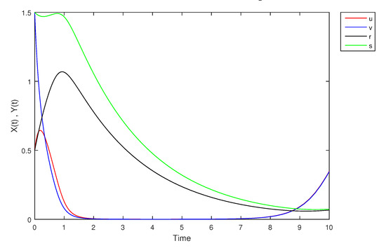
Figure 10. The solution of (7) at $\alpha$ = 0.0 for short time period.

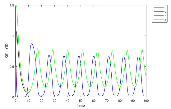
Figure 11. The solution of (7) at $\alpha$ = 0.0 as time increases.

At $\alpha$-level = 0.5, the solution is shown in Figure 12 and Figure 13.

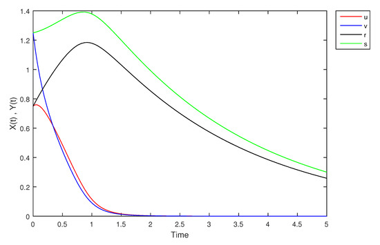
Figure 12. The solution of (7) at $\alpha$ = 0.5 for short time period.

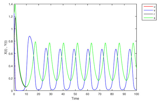
Figure 13. The solution of (7) at $\alpha$ = 0.5 as time increases.

At $\alpha$-level = 1, the solution is shown in Figure 14:

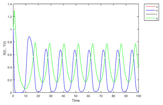
Figure 14. The solution of (7) at $\alpha$=1.

In this case (2-2) solution, the lower and upper limits for $X\left(t\right)$ and $Y\left(t\right)$ start at different values up to time $t<15$ with $v\left(t\right)>u\left(t\right)$ and $s\left(t\right)>r\left(t\right)$. As time increases they coincide as shown in the figures. The crisp solution lies between them.

In general and from the above cases, we obtain biologically unacceptable and unstable solution when $X\left(t\right)$and$Y\left(t\right)$ are (1,1), (1,2), (2,1)-differentiable for $\alpha <1$, while at $\alpha =1$the solution is equivalent to the crisp case. When $X\left(t\right)$and$Y\left(t\right)$are (2)-differentiable, we notice that as $t\to \infty$ the solution becomes periodic and stable.

Now, we try to use a triangular fuzzy numbers with small supports for the initial conditions. let $x_0=y_0=(0.9999,1,1.0001)$ then ${\left[x_0\right]}_{\alpha }={\left[y_0\right]}_{\alpha }$=[$0.9999+\frac{\alpha }{10000},1.0001-\frac{\alpha }{10000}$]. Since the model when $X\left(t\right)$and$Y\left(t\right)$are (2)-differentiable give a fuzzy solution which is biologically acceptable we find the solution of $X\left(t\right)$and$Y\left(t\right)$ when they are (2)-differentiable at $\alpha -level=0.$ Therefore, we have the following model:

$$\begin{array}{ccc}\hfill u^{\prime }& =& 2v-2u^2-r{tan}^{-1}\left(5u\right),\hfill \\ \hfill v^{\prime }& =& 2u-2v^2-s{tan}^{-1}\left(5v\right),\hfill \\ \hfill r^{\prime }& =& -0.4r+0.6s{tan}^{-1}\left(5v\right),\hfill \\ \hfill s^{\prime }& =& -0.4s+0.6r{tan}^{-1}\left(5u\right),\hfill \\ \hfill u_0& =& r_0=0.9999+\frac{\alpha }{10000}\mathrm{and}{v}_0=s_0=1.0001-\frac{\alpha }{10000},\hfill \end{array}$$

(9)

The solution is shown in Figure 15 and Figure 16:

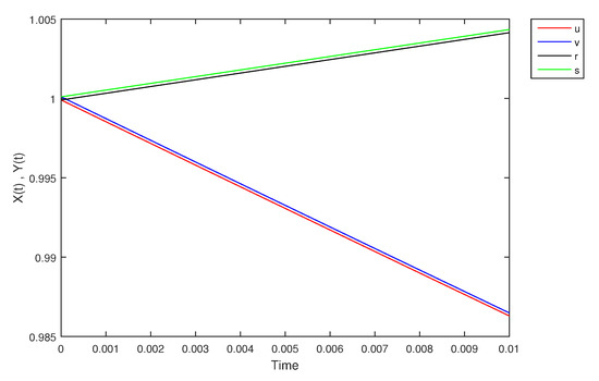
Figure 15. The solution of (8) at $\alpha$ = 0.0 for short time period.

Figure 16. The solution of (8) at $\alpha$ = 0.0 as time increases.

We see that initially $v\left(t\right)>u\left(t\right)$and$s\left(t\right)>r\left(t\right)$ but as $t\to \infty$ the solution becomes periodic and stable and $v\left(t\right)=u\left(t\right)$and$s\left(t\right)=r\left(t\right)$. So, the solution of (8) is better than the previous one (using initial conditions with large supports).

3.2. Fuzzy Parameters

In this part, we try to see what may happen when we make the parameters of the model (2) triangular fuzzy numbers.

For example, let $r=\left(1,2,3\right)$ with ${\left[r\right]}_{\alpha }=\left[1+\alpha ,3-\alpha \right],a=\left(4,5,6\right)$with ${\left[a\right]}_{\alpha }=\left[4+\alpha ,6-\alpha \right]$, $D=\left(0.2,0.4,0.6\right)$with${\left[D\right]}_{\alpha }=[0.2$+$\frac{\alpha }{5},0.6-\frac{\alpha }{5}]$ and $s=\left(0.4,0.6,0.8\right)$ with${\left[s\right]}_{\alpha }=\left[0.4+\frac{\alpha }{5},0.8-\frac{\alpha }{5}\right].$ Then (2) becomes:

$$\begin{array}{ccc}\hfill X^{{}^{\prime }}\left(t\right)& =& \left(1,2,3\right)X\left(1-X\right)-Y{tan}^{-1}\left(\left(4,5,6\right)X\right),\hfill \\ \hfill Y^{\prime }\left(t\right)& =& -\left(0.2,0.4,0.6\right)Y+\left(0.4,0.6,0.8\right)Y{tan}^{-1}\left(5X\right),\hfill \\ \hfill x_0& =& \left(0.5,1,1.5\right)\mathrm{and}{y}_0=\left(0.5,1,1.5\right).\hfill \end{array}$$

(10)

(1)

If X and Y are (1)-differentiable, then we have the following model:

$$\begin{array}{ccc}\hfill u^{\prime }& =& (1+\alpha )u-(3-\alpha )v^2-s{tan}^{-1}\left((6-\alpha )v\right),\hfill \\ \hfill v^{\prime }& =& (3-\alpha )v-(1+\alpha )u^2-r{tan}^{-1}\left((4+\alpha )u\right),\hfill \\ \hfill r^{\prime }& =& -(0.6-\frac{\alpha }{5})s+(0.4+\frac{\alpha }{5})r{tan}^{-1}\left((4+\alpha )u\right),\hfill \\ \hfill s^{\prime }& =& -(0.2+\frac{\alpha }{5})r+(0.8-\frac{\alpha }{5})s{tan}^{-1}\left((6-\alpha )v\right),\hfill \\ \hfill u_0& =& r_0=0.5+\frac{\alpha }{2}\mathrm{and}{v}_0=s_0=1.5-\frac{\alpha }{2}\hfill \end{array}$$

(11)

The equilibrium points of (9) are ${\chi }_{(0,0)},{\chi }_{(1,0)}.$

At $\alpha -level=0$, the solution is shown in Figure 17:

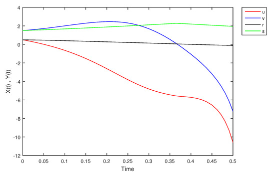Figure 17. The solution of (10) at $\alpha$ = 0.0.

At $\alpha$-level = 0.5, the solution is shown in Figure 18:

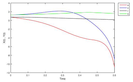Figure 18. The solution of (10) at $\alpha$ = 0.5.

At $\alpha$-level = 1, the solution is shown in Figure 19:

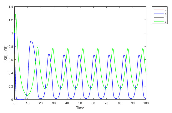Figure 19. The solution of (10) at $\alpha$ = 1.

(2)

If X is (1)-differentiable and Y is (2)-differentiable, then we have the following model:

$$\begin{array}{ccc}\hfill u^{\prime }& =& (1+\alpha )u-(3-\alpha )v^2-s{tan}^{-1}\left((6-\alpha )v\right),\hfill \\ \hfill v^{\prime }& =& (3-\alpha )v-(1+\alpha )u^2-r{tan}^{-1}\left((4+\alpha )u\right),\hfill \\ \hfill r^{\prime }& =& -(0.2+\frac{\alpha }{5})r+(0.8-\frac{\alpha }{5})s{tan}^{-1}\left((6-\alpha )v\right),\hfill \\ \hfill s^{\prime }& =& -(0.6-\frac{\alpha }{5})s+(0.4+\frac{\alpha }{5})r{tan}^{-1}\left((4+\alpha )u\right),\hfill \\ \hfill u_0& =& r_0=0.5+\frac{\alpha }{2}\mathrm{and}{v}_0=s_0=1.5-\frac{\alpha }{2}.\hfill \end{array}$$

(12)

At $\alpha$-level = 0, the solution is shown in Figure 20:

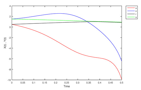Figure 20. The solution of (11) at $\alpha$ = 0.0.

At $\alpha$-level = 0.5, the solution is in Figure 21:

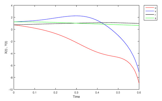Figure 21. The solution of (11) at $\alpha$ = 0.5.

At $\alpha$-level = 1, the solution is shown in Figure 22:

Figure 22. The solution of (10) at $\alpha$ = 1.

(3)

If X is (2)-differentiable and Y is (1)-differentiable, then we have the following model:

$$\begin{array}{ccc}\hfill u^{\prime }& =& (3-\alpha )v-(1+\alpha )u^2-r{tan}^{-1}\left((4+\alpha )u\right),\hfill \\ \hfill v^{\prime }& =& (1+\alpha )u-(3-\alpha )v^2-s{tan}^{-1}\left((6-\alpha )v\right),\hfill \\ \hfill r^{\prime }& =& -(0.6-\frac{\alpha }{5})s+(0.4+\frac{\alpha }{5})r{tan}^{-1}\left((4+\alpha )u\right),\hfill \\ \hfill s^{\prime }& =& -(0.2+\frac{\alpha }{5})r+(0.8-\frac{\alpha }{5})s{tan}^{-1}\left((6-\alpha )v\right),\hfill \\ \hfill u_0& =& r_0=0.5+\frac{\alpha }{2}\mathrm{and}{v}_0=s_0=1.5-\frac{\alpha }{2}.\hfill \end{array}$$

(13)

At $\alpha$-level = 0, the solution is shown in Figure 23:

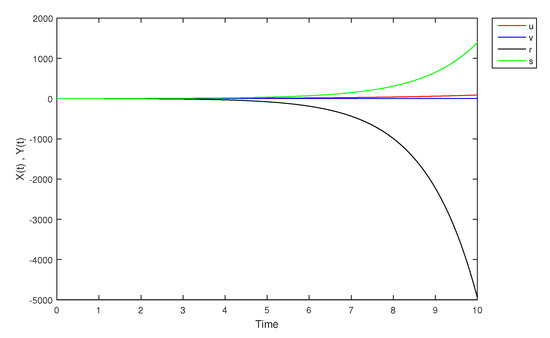Figure 23. The solution of (12) at $\alpha$ = 0.0.

At $\alpha$-level = 0.5, the solution is shown in Figure 24:

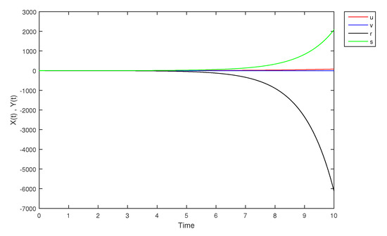Figure 24. The solution of (12) at $\alpha$ = 0.5.

At $\alpha$-level = 1, the solution is shown in Figure 25:

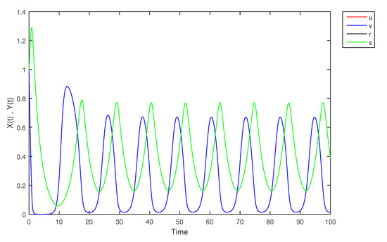Figure 25. The solution of (12) at $\alpha$ = 1.

(4)

If X and Y are (2)-differentiable, then we have the following model:

$$\begin{array}{ccc}\hfill u^{\prime }& =& (3-\alpha )v-(1+\alpha )u^2-r{tan}^{-1}\left((4+\alpha )u\right),\hfill \\ \hfill v^{\prime }& =& (1+\alpha )u-(3-\alpha )v^2-s{tan}^{-1}\left((6-\alpha )v\right),\hfill \\ \hfill r^{\prime }& =& -(0.2+\frac{\alpha }{5})r+(0.8-\frac{\alpha }{5})s{tan}^{-1}\left((6-\alpha )v\right),\hfill \\ \hfill s^{\prime }& =& -(0.6-\frac{\alpha }{5})s+(0.4+\frac{\alpha }{5})r{tan}^{-1}\left((4+\alpha )u\right),\hfill \\ \hfill u_0& =& r_0=0.5+\frac{\alpha }{2}\mathrm{and}{v}_0=s_0=1.5-\frac{\alpha }{2}.\hfill \end{array}$$

(14)

At $\alpha$-level = 0, the solution is shown in Figure 26, Figure 27 and Figure 28:

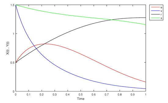
Figure 26. The solution of (13) at $\alpha$ = 0.0 for a short time period.

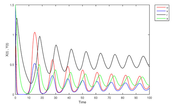
Figure 27. The solution of (13) at $\alpha$ = 0.0 as time increases.

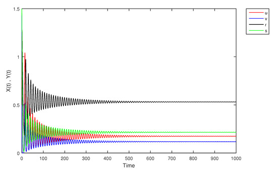
Figure 28. The solution of (13) at $\alpha$ = 0.0 as time increases.

At $\alpha$-level = 0, the solution is unstable since $ast\to \infty ,u\left(t\right)\to 0.1744,v\left(t\right)\to 0.1179,r\left(t\right)\to 0.5308,s\left(t\right)\to 0.2155.$

$\alpha$-level = 0.5 is shown in Figure 29 and Figure 30:

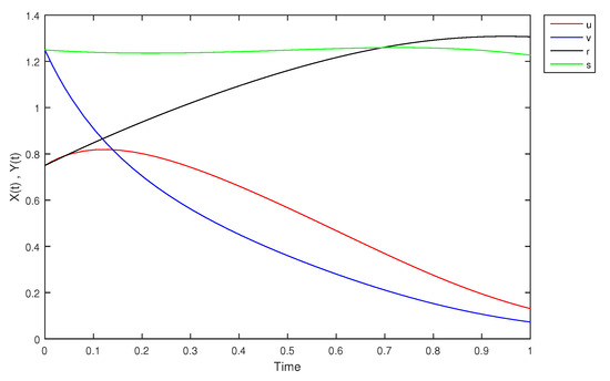
Figure 29. The solution of (13) at $\alpha$ = 0.5 for a short time period.

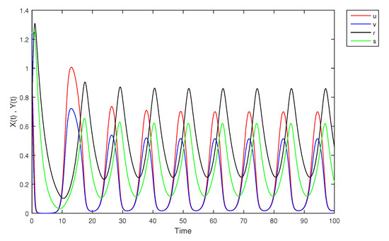
Figure 30. The solution of (13) at $\alpha$ = 0.5 as time increases.

At $\alpha$-level = 1, the solution is shown in Figure 31:

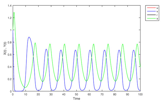
Figure 31. The solution of (13) at $\alpha$ = 1.

Now, we want to fuzzify the parameters of the model (2) using triangular fuzzy number with small support, as follows:

Let

$$\begin{array}{ccc}\hfill r& =& \left(1.9995,2,2.0005\right)\mathrm{with}{\left[r\right]}_{\alpha }=\left[1.9995+\frac{\alpha }{2000},2.0005-\frac{\alpha }{2000}\right],\hfill \\ \hfill a& =& \left(4.9995,5,5.0005\right)\mathrm{with}{\left[a\right]}_{\alpha }=\left[4.9995+\frac{\alpha }{2000},5.0005-\frac{\alpha }{2000}\right],\hfill \\ \hfill D& =& \left(0.3995,0.4,0.4005\right)\mathrm{with}{\left[D\right]}_{\alpha }=\left[0.3995+\frac{\alpha }{2000},0.4005-\frac{\alpha }{20000}\right],\hfill \\ \hfill s& =& \left(0.5995,0.6,0.6005\right)\mathrm{with}{\left[s\right]}_{\alpha }=\left[0.5995+\frac{\alpha }{2000},0.6005-\frac{\alpha }{2000}\right],\hfill \\ \hfill x_0& =& \left(0.9995,1,1.0005\right)\mathrm{with}{\left[x_0\right]}_{\alpha }=\left[0.9995+\frac{\alpha }{2000},1.0005-\frac{\alpha }{2000}\right],\hfill \\ \hfill y_0& =& \left(0.9995,1,1.0005\right)\mathrm{with}{\left[y_0\right]}_{\alpha }=\left[0.9995+\frac{\alpha }{2000},1.0005-\frac{\alpha }{2000}\right].\hfill \end{array}$$

Then we have the following model:

$$\begin{array}{ccc}\hfill X^{\prime }\left(t\right)& =& \left(1.9995,2,2.0005\right)X\left(1-X\right)-Y{tan}^{-1}\left(\left(4.9995,5,5.0005\right)X\right),\hfill \\ \hfill Y^{\prime }\left(t\right)& =& -\left(0.3995,0.4,0.4005\right)Y+\left(0.5995,0.6,0.6005\right)Y{tan}^{-1}\left(5X\right),\hfill \\ \hfill x_0& =& \left(0.9995,1,1.0005\right)\mathrm{and}{y}_0=\left(0.9995,1,1.0005\right).\hfill \end{array}$$

(15)

We solve model (14) when X and Y are (2)-differentiable, then it becomes as follows:

$$\begin{array}{ccc}\hfill u^{\prime }& =& (2.0005-\frac{\alpha }{2000})v-(1.9995+\frac{\alpha }{2000})u^2-r{tan}^{-1}\left((4.9995+\frac{\alpha }{2000})u\right),\hfill \\ \hfill v^{\prime }& =& (1.9995+\frac{\alpha }{2000})u-(2.0005-\frac{\alpha }{2000})v^2-s{tan}^{-1}\left((5.0005-\frac{\alpha }{2000})v\right),\hfill \\ \hfill r^{\prime }& =& -(0.3995+\frac{\alpha }{2000})r+(0.6005-\frac{\alpha }{2000})s{tan}^{-1}\left((5.0005-\frac{\alpha }{2000})v\right),\hfill \\ \hfill s^{\prime }& =& -(0.4005-\frac{\alpha }{2000})s+(0.5995+\frac{\alpha }{2000})r{tan}^{-1}\left((4.9995+\frac{\alpha }{2000})u\right),\hfill \\ \hfill u_0& =& r_0=0.9995+\frac{\alpha }{2000}\mathrm{and}{v}_0=s_0=1.0005-\frac{\alpha }{2000}\hfill \end{array}$$

(16)

At $\alpha$-level$=0$, the solution is shown in Figure 32 and Figure 33:

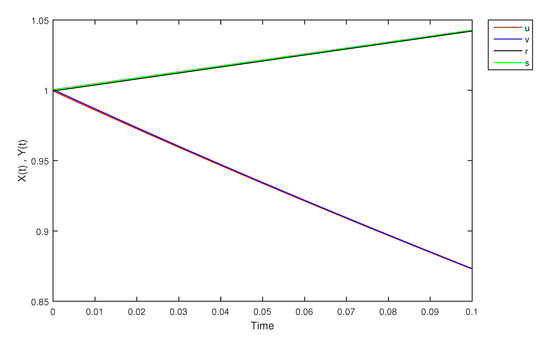
Figure 32. The solution of (14) at $\alpha$ = 0.0 for a short time period.

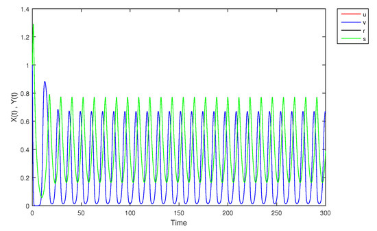
Figure 33. The solution of (14) at $\alpha$ = 0.0 as time increases.

When we fuzzify the parameters of (2) by triangular fuzzy numbers, then for $\alpha <1$we obtain unacceptable solutions when X and Y are (1,1), (1,2), (2,1)-differentiable. While, when X and Y are (2)-differentiable, the solution is unstable at $\alpha -level=0,$ but it becomes periodic as $\alpha$ increases for $\alpha <1$ with $u\left(t\right)>v\left(t\right)$and$r\left(t\right)>s\left(t\right).$ So, there are no fuzzy solution for X and Y. However, at $\alpha =1$the solution is equivalent to the crisp case for all derivative forms of X and Y. When we use triangular fuzzy numbers of small supports, then the solution when X and Y are (2)-differentiable at $\alpha =0$ is periodic and stable. Therefore, as $t\to \infty ,r\left(t\right)>s\left(t\right)$ so there is no fuzzy solution for Y.

4. Conclusions

We constructed a fuzzy predator-prey model with functional response. We fuzzified the initial conditions and the parameters. We also considered triangular fuzzy numbers. The resulting systems are then solved numerically using the fuzzy Runge-Kutta method. The results obtained were not always better than the crisp one. The (1-1), (1-2) and the (2-1) solution were not acceptable and are incompatible with biological facts. While the (2-2) solutions are stable, periodic and are biologically meaningful. For the triangular fuzzy numbers, it is better to use triangular fuzzy numbers with small supports since they produce periodic and stable solutions. Fuzzy parameters didn’t lead to good solutions that are acceptable and in agreement with fuzzy logic.

References

- Bede, B.; Gal, G.S. Generalizations of differentiability of fuzzy number valued functions with applications to fuzzy differential equations. Fuzzy Sets Syst. 2005, 151, 581–599. [Google Scholar] [CrossRef]
- Bede, B.; Stefanini, L. Solution of Fuzzy Differential Equations with Generalized Differentiability Using LU-Parametric Representation; Atlantis Press: Atlantis, France, 2011. [Google Scholar]
- Bede, B.; Stefanini, L. Generalized differentiability of fuzzy-valued function. Fuzzy Sets Syst. 2012, 230, 119–141. [Google Scholar] [CrossRef]
- Cano, Y.C.; Flores, H.R. On new solutions of fuzzy differential equations. Chaos Solitons Fractals 2008, 38, 112–119. [Google Scholar] [CrossRef]
- Gomes, L.T.; Barros, L.C. A note on the generalized difference and the generalized differentiability. Fuzzy Sets Syst. 2015, 280, 142–145. [Google Scholar] [CrossRef]
- Pirzada, U.M.; Vakaskar, D.C. Existence of Hukuhara differentiability of fuzzy-valued functions. J. Indian Math. 2017, 84, 239–254. [Google Scholar] [CrossRef]
- Stefanini, L. A generalization of Hukuhara difference for interval and fuzzy arithmetic. Fuzzy Sets Syst. 2008, 161, 1564–1584. [Google Scholar] [CrossRef]
- Bede, B.; Gal, S.G. Solutions of fuzzy differential equations based on generalized differentiability. Commun. Math. Anal. 2010, 9, 22–41. [Google Scholar]
- Ortega, N.R.; Sallum, P.C.; Massad, E. Fuzzy Dynamical Systems in Epidemic Modeling. Kybernetes 2000, 29, 201–218. [Google Scholar] [CrossRef]
- Ahmad, M.Z.; Baets, B. A Predator-Prey Model with Fuzzy Initial Populations. In Proceedings of the 13th IFSA World Congress and 6th EUSFLAT Conference, Lisbon, Portugal, 20–24 July 2009; pp. 1311–1314. [Google Scholar]
- Ahmad, M.Z.; Hasan, M.K. Modeling of Biological Populations Using Fuzzy Differential Equations. Intern. J. Mod. Physic Conf. Ser. 2012, 9, 354–363. [Google Scholar] [CrossRef]
- Ghanaie, Z.A.; Moghadam, M. Solving fuzzy differential equations by Runge-Kutta method. J. Math. Comput. Sci. 2011, 2, 295–306. [Google Scholar]
- Ma, M.; Friedman, M.; Kandel, A. Numerical solutions of fuzzy differential equations. Fuzzy Sets Syst. 1999, 105, 133–138. [Google Scholar] [CrossRef]
- Attili, B. The Shooting Method for Solving Second Order Fuzzy Two-Point Boundary Value Problems. Intern. J. Appl. Math. 2019, 32, 663–676. [Google Scholar] [CrossRef][Green Version]
- Attili, B. Initial Value Methods for the Numerical Simulation of Fuzzy Two-Point Boundary Value Problems using General Linear Method. Intern. J. Fuzzy Syst. Appl. 2021, 10, 94–126. [Google Scholar]
- Mallak, S.; Bedo, D.A. Fuzzy Comparison Method for Particular Fuzzy Numbers. J. Mahani Math. Res. Cent. 2013, 3, 1–14. [Google Scholar]
- Akin, O.; Oruc, O. A Prey Predator Model with Fuzzy Initial Values. Hacet. J. Math. Stat. 2012, 4, 387–395. [Google Scholar]
- Mizukoshi, M.T.; Barros, L.C.; Bassanezi, R.C. Stability of Fuzzy Dynamic Systems. Int. J. Uncertain. Fuzziness Knowl. Based Syst. 2009, 17, 69–83. [Google Scholar] [CrossRef]
- Peixoto, M.S.; Barros, L.C.; Bassanezi, R.C. Predator-Prey Fuzzy Model. Ecol. Model 2008, 214, 39–44. [Google Scholar] [CrossRef]
- Attili, B.; Mallak, S. Existence of Limit Cycles in A Predator-Prey System with a Functional Responce of the Form Arctan(ax). Commun. Math. Anal. 2006, 1, 27–33. [Google Scholar]
- Pereira, C.M.; Cecconello, M.S.; Bassanezi, R.C. Prey-Predator Model Under Fuzzy Uncertanties. In Fuzzy Information Processing. NAFIPS 2018. Communications in Computer and Information Science; Barreto, G., Coelho, R., Eds.; Springer: Berlin/Heidelberg, Germany, 2018; Volume 831. [Google Scholar]
- Barzinji, K. Numerical Solution of Fuzzy Delay Predator-Prey System. Intern. J. Math. Anal. 2017, 11, 595–603. [Google Scholar] [CrossRef]
- Banerjee, M.; Mukherjee, N.; Volpert, V. Prey-Predator Model with a Nonlocal Bistable Dynamics of Prey. Mathematics 2018, 6, 41. [Google Scholar] [CrossRef]
- Pal, D.; Mahapatra, G.S.; Samanta, G.P. Stability and bionomic analysis of fuzzy prey–predator harvesting model in presence of toxicity: A dynamic approach. Bull. Math. Biol. 2016, 78, 1493–1519. [Google Scholar] [CrossRef] [PubMed]
- Yavuz, M.; Sene, N. Stability Analysis and Numerical Computation of the Fractional Predator–Prey Model with the Harvesting Rate. Fractal Fract. 2020, 4, 35. [Google Scholar] [CrossRef]
- Yu, X.; Yuan, S.; Zhang, T. About the optimal harvesting of a fuzzy predator–prey system: A bioeconomic model incorporating prey refuge and predator mutual interference. Nonlinear Dyn. 2018, 94, 2143–2160. [Google Scholar] [CrossRef]
- Pal, D.; Mahapatra, G.S.; Mahato, S.K.; Samanta, G.P. A Mathematical Model of A Prey-Predator Type Fishery in the Presence of Toxicity With Fuzzy Optimal Harvisting. J. Appl. Math. Inform. 2020, 38, 13–36. [Google Scholar] [CrossRef]
- Thota, S. A Mathematical Study on a Diseased Prey-Predator Model with Predator Harvesting. Asian J. Fuzzy Appl. Math. 2020, 8, 16–21. [Google Scholar] [CrossRef]
- Zimmerman, H.J. Fuzzy Set Theory and Its Applications, 4th ed.; Springer: Berlin/Heidelberg, Germany, 2006. [Google Scholar]
- Mallak, S.; Bedo, D. Particular Fuzzy Numbers and a Fuzzy Comparison Method between Them. Intern. J. Fuzzy Math. Syst. 2013, 2, 113–123. [Google Scholar]
Publisher’s Note: MDPI stays neutral with regard to jurisdictional claims in published maps and institutional affiliations. |
© 2021 by the authors. Licensee MDPI, Basel, Switzerland. This article is an open access article distributed under the terms and conditions of the Creative Commons Attribution (CC BY) license (https://creativecommons.org/licenses/by/4.0/).