A Nonhomogeneous Boundary Value Problem for Steady State Navier-Stokes Equations in a Multiply-Connected Cusp Domain

Abstract

The boundary value problem for the steady Navier–Stokes system is considered in a $2D$ multiply-connected bounded domain with the boundary having a power cusp singularity at the point O. The case of a boundary value with nonzero flow rates over connected components of the boundary is studied. It is also supposed that there is a source/sink in O. In this case the solution necessarily has an infinite Dirichlet integral. The existence of a solution to this problem is proved assuming that the flow rates are “sufficiently small”. This condition does not require the norm of the boundary data to be small. The solution is constructed as the sum of a function with the finite Dirichlet integral and a singular part coinciding with the asymptotic decomposition near the cusp point.

1. Introduction

In the paper we study the nonhomogeneous stationary boundary value problem for the Navier-Stokes equations

$$\left\{\begin{array}{cccc}\hfill -\nu \Delta \mathbf{u}+(\mathbf{u}·\nabla )\mathbf{u}+\nabla p& =\mathbf{f},\hfill & \hfill & x\in \mathsf{\Omega },\hfill \\ \hfill \mathrm{div}\mathbf{u}& =0,\hfill & \hfill & x\in \mathsf{\Omega },\hfill \\ \hfill \mathbf{u}& =\mathbf{a},\hfill & \hfill & x\in \partial \mathsf{\Omega },\hfill \end{array}\right.$$

(1)

in a multiply-connected domain $\mathsf{\Omega }\subset {\mathbb{R}}^2$ with a cusp point $O=(0,0)$ on the boundary. We assume that $\partial \mathsf{\Omega }={\cup }_{j=1}^N{\mathsf{\Gamma }}_j\cup \mathsf{\Gamma }$ consists of $N+1$ disjoint components $\mathsf{\Gamma },$${\mathsf{\Gamma }}_j,$$j=1,...,N,$

$$\mathsf{\Omega }={\mathsf{\Omega }}_0\cup G=\left(D_0\backslash \left({\cup }_{j=1}^N{\overline{D}}_j\right)\right)\cup G,{\overline{D}}_j\subset D_0,j=1,\dots ,N,$$

where ${\mathsf{\Gamma }}_j=\partial D_j,j=1,\dots ,N,$$\mathsf{\Gamma }=\partial \mathsf{\Omega }\backslash {\cup }_{j=1}^N{\mathsf{\Gamma }}_j$ and $G=\{x\in {\mathbb{R}}^2:|x_1|\le \phi \left(x_2\right),x_2\in (0,H]\},$$\phi \left(x_2\right)={\gamma }_0{x}_2^{\lambda },{\gamma }_0=\mathrm{const},\lambda >1.$ Moreover, we suppose that $\partial \mathsf{\Omega }\cap \partial {\mathsf{\Omega }}_0$ is $C^2$ (see Figure 1). In (1) the velocity vector $\mathbf{u}$ and the pressure function p are the unknowns while the boundary value $\mathbf{a}\in W^{1/2,2}(\partial \mathsf{\Omega })$ and the external force $\mathbf{f}\in L^2\left(\mathsf{\Omega }\right)$ are given; $\nu >0$ denotes a constant coefficient of the kinematic viscosity.

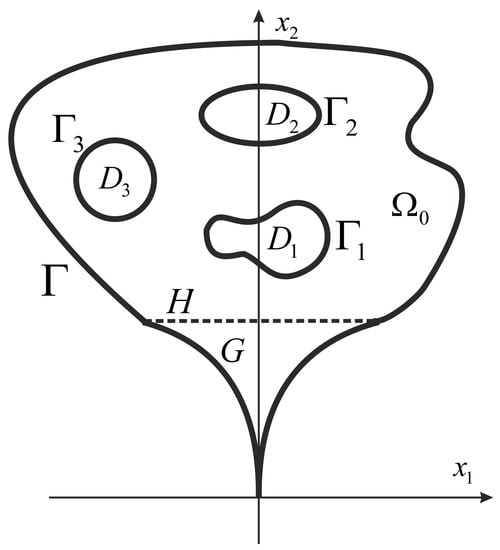
Figure 1. Domain $\mathsf{\Omega }={\mathsf{\Omega }}_0\cup G$.

We assume that the support of $\mathbf{a}$ is separated from the cusp point O, i.e.,

$$\mathrm{supp}\mathbf{a}\subset \left(\mathsf{\Gamma }\cap \partial {\mathsf{\Omega }}_0\right)\cup \left({\cup }_{j=1}^N{\mathsf{\Gamma }}_j\right).$$

Let

$$\begin{array}{c}{F}_0=\underset{\mathsf{\Gamma }\cap \partial {\mathsf{\Omega }}_0}{\int }\mathbf{a}·\mathbf{n}dS,F_j=\underset{{\mathsf{\Gamma }}_j}{\int }\mathbf{a}·\mathbf{n}dS,j=1,\dots ,N,\end{array}$$

(2)

be the flow rates of the boundary value $\mathbf{a}$ over the outer boundary $\mathsf{\Gamma }\cap \partial {\mathsf{\Omega }}_0$ and the inner boundaries ${\mathsf{\Gamma }}_j,$$j=1,\dots ,N,$ where $\mathbf{n}$ denotes the unit vector of the outward normal to $\partial \mathsf{\Omega }$. By the incompressibility of the fluid it follows that

$$\begin{array}{c}\underset{\sigma \left(R\right)}{\int }\mathbf{u}·\mathbf{n}dS=-\left(F_0+{\displaystyle \sum _{j=1}^N}{F}_j\right),0<R<H,\end{array}$$

(3)

where $\sigma \left(R\right)=(-\phi (R),\phi (R\left)\right)$ is a cross section of G by the straight line $x_2=R$ parallel to the $x_1$-axis. We assume that the total flux may be nonzero, i.e., $F_0+{\displaystyle \sum _{j=1}^N}{F}_j\ne 0$. This nonzero condition means that there is a source or sink in the cusp point O. Then, due to the geometry of the domain, the velocity vector field $\mathbf{u}$ necessarily has infinite Dirichlet integral $\underset{\mathsf{\Omega }}{\int }{|\nabla \mathbf{u}\left(x\right)|}^{2}dx=\infty$ (see, e.g., [1]).

The point source/sink approach is widely used in physics, astronomy and in fluid and aerodynamics. The behaviour of solutions to the Stokes and Navier–Stokes equations in singularly perturbed domains became of growing interest during the last fifty years. There is an extensive literature concerning these issues for various elliptic problems, e.g., [2,3,4,5,6,7,8,9,10,11,12,13,14,15,16,17,18]. In particular, the steady Navier–Stokes equations are studied in a punctured domain $\mathsf{\Omega }={\mathsf{\Omega }}_0\backslash \left\{O\right\}$ with $O\in {\mathsf{\Omega }}_0$ assuming that the point O is a sink or source of the fluid [19,20,21] (see also [22] for the review of these results). We also mention the papers [23,24,25] where the existence of a solution (with an infinite Dirichlet integral) to the Navier–Stokes problem with a sink or source in the cusp point O was proved for arbitrary data and the papers [26,27,28] where the asymptotics of a solution to the nonstationary Stokes problem is studied in domains with conical points and conical outlets to infinity.

The existence of singular solutions to the time-periodic and initial boundary value problems for the linear Stokes and the nonlinear Navier–Stokes equations in domains with a cusp point on the boundary were studied in recent papers [29,30,31,32], where the case with a sink/source in the cusp point O was considered. In [23], the existence of a generic stationary solution with infinite Dirichlet integral was proved. However, the behaviour of the solution near the cusp point was not found. The asymptotic decomposition near the cusp point of the solution $\mathbf{u}$ to problem (1) was constructed and the existence of a unique solution which is represented as a sum of this decomposition and a vector field belonging to a suitable second order weighted Sobolev space is proved in [1]. In [1], it is assumed that $\mathbf{a}\in W^{3/2,2}(\partial \mathsf{\Omega })$ and the results are obtained under the condition that the norm ${\parallel \mathbf{a}\parallel }_{W^{3/2,2}(\partial \mathsf{\Omega })}$ is sufficiently small.

In this paper we extend the results of [1] in two directions: first, we study the case of domains with multiply-connected boundaries and, second, we prove the existence of the solution coinciding near the cusp point with the formal asymptotic decomposition assuming only that the flow rates $F_0,F_1,\dots ,F_N$ of the boundary value $\mathbf{a}$ are sufficiently small. The proof is based on the construction of an extension of the boundary value which coincides near the cusp point with the asymptotic decomposition and allows to obtain needed a priori estimates assuming only that flow rates are sufficiently small. Note that in this case the norm of $\mathbf{a}$ is not obliged to be small. It is worth to mention the papers [33,34,35] where the nonhomogeneous boundary value problem for the stationary Navier–Stokes equations was studied in bounded domains with multiply-connected boundaries having $C^2$-regularity.

2. Notation and Auxiliary Results

2.1. Function Spaces

We will use the letter “c” for a generic constant which numerical value or dependence on parameters is unessential to our considerations; “c” may have different values in a single computation. Vector valued functions are denoted by bold letters while function spaces for scalar and vector valued functions are denoted in the same way.

Let D be a bounded domain in ${\mathbb{R}}^n$ with Lipschitz boundary. $C^{\infty }\left(D\right)$ denotes the set of all infinitely differentiable in D functions and $C_0^{\infty }\left(D\right)$ is the subset of all functions from $C^{\infty }\left(D\right)$ with compact supports in D. For given non-negative integers k and $q>1$, $L^q\left(D\right)$ and $W^{k,q}\left(D\right)$ denote the usual Lebesgue and Sobolev spaces; $W^{k-1/q,q}(\partial D)$ is the trace space on $\partial D$ of functions from $W^{k,q}\left(D\right)$. ${\mathring{W}}^{1,2}\left(D\right)$ is the closure of $C_0^{\infty }\left(D\right)$ in $W^{1,2}$-norm. $J_0^{\infty }\left(D\right)$ is the set of all solenoidal $(\mathrm{div}\mathbf{u}=0)$ vector fields $\mathbf{u}$ from $C_0^{\infty }\left(D\right)$ and $H\left(D\right)$ is the closure of $J_0^{\infty }\left(D\right)$ in the gradient norm ${\parallel \nabla ·\parallel }_{L^2\left(D\right)}$.

Lemma 1

([36,37], Chapter 1, Lemma 1). Let $D\subset {\mathbb{R}}^2$ be a bounded domain. If $u\in W^{1,2}\left(D\right),$ then the following estimate

$${\parallel u\parallel }_{L^4\left(D\right)}^4\le {c\parallel u\parallel }_{W^{1,2}\left(D\right)}^2{\parallel u\parallel }_{L^2\left(D\right)}^2\le c{\parallel u\parallel }_{W^{1,2}\left(D\right)}^4$$

holds. Moreover, if $u\in {\mathring{W}}^{1,2}\left(D\right)$ then

$${\parallel u\parallel }_{L^4\left(D\right)}^4\le {2\parallel u\parallel }_{L^2\left(D\right)}^2{\parallel \nabla u\parallel }_{L^2\left(D\right)}^2\le c{\parallel \nabla u\parallel }_{L^2\left(D\right)}^4.$$

Consider the domain $\mathsf{\Omega }$ with a cusp point. We introduce a family of subdomains ${\mathsf{\Omega }}_k\subset \mathsf{\Omega }$ with Lipschitz boundaries:

$${\mathsf{\Omega }}_k={\mathsf{\Omega }}_{k-1}\cup \{x\in {\mathbb{R}}^2:|x_1|\le \phi \left(x_2\right),x_2\in (h_k,h_{k-1})\}={\mathsf{\Omega }}_{k-1}\cup {\omega }_k,$$

where

$$h_0=H,h_k=h_{k-1}-\frac{\phi \left(h_{k-1}\right)}{2L},k=1,2,\dots ,$$

(4)

and L is the Lipschitz constant for the function $\phi$.

We write $u\in W_{loc}^{l,q}(\overline{\mathsf{\Omega }}\backslash \left\{O\right\})$ if $u\in W^{l,q}\left({\mathsf{\Omega }}_k\right)$ for $\forall k.$

Lemma 2.

Let $u\in W_{loc}^{1,2}(\overline{\mathsf{\Omega }}\backslash \left\{O\right\})$, $u=0$ on $\partial \mathsf{\Omega }\backslash \left\{O\right\}$. If $\underset{G}{\int }|\phi \left(x_2\right){|}^{2\alpha }{|\nabla u\left(x\right)|}^{2}dx<\infty ,$ then the integral $\underset{G}{\int }|\phi \left(x_2\right){|}^{2\alpha -2}{\left|u\left(x\right)\right|}^{2}dx$ is finite and the following inequality

$$\begin{array}{c}\underset{H_1}{\overset{H_2}{\int }}\underset{-\phi \left(x_2\right)}{\overset{\phi \left(x_2\right)}{\int }}|\phi \left(x_2\right){|}^{\alpha -2}|u\left(x\right){|}^{2}d{x}_{1}d{x}_2\le \frac{4}{{\pi }^2}\underset{H_1}{\overset{H_2}{\int }}\underset{-\phi \left(x_2\right)}{\overset{\phi \left(x_2\right)}{\int }}|\phi \left(x_2\right){|}^{\alpha }{|\nabla u\left(x\right)|}^{2}d{x}_{1}d{x}_2\end{array}$$

(5)

holds, where $H_1,H_2$ are any numbers from the interval $[0,H]$

The proof of this lemma can be found in [32] (see Lemma 2.1).

2.2. Formal Asymptotic Decomposition

The formal asymptotic decomposition $\left({\mathbf{U}}^{\left[J\right]},P^{\left[J\right]}\right)$ of the solution $(\mathbf{u},p)$ of problem (1) near the cusp point O was constructed in [1]. It has the form

$$\begin{array}{cc}\hfill U_1^{\left[J\right]}(y_1,y_2)=& y_2^{-1}{\mathcal{U}}_{1,0}\left(y_1\right)+{\displaystyle \sum _{k=1}^J}{y}_2^{-1+k(\lambda -1)}{\mathcal{U}}_{1,k}\left(y_1\right),\hfill \\ \hfill U_2^{\left[J\right]}(y_1,y_2)=& {\displaystyle \frac{\mathbb{F}}{{\kappa }_0}}{y}_2^{-\lambda }\mathsf{\Phi }\left(y_1\right)+{\displaystyle \sum _{k=1}^J}{y}_2^{-\lambda +k(\lambda -1)}{\mathcal{U}}_{2,k}\left(y_1\right),\hfill \\ \hfill P^{\left[J\right]}(y_1,y_2)=& {\displaystyle \frac{\mathbb{F}}{{\kappa }_0(1-3\lambda )}}{y}_2^{1-3\lambda }+y_2^{-1-\lambda }{\mathcal{Q}}_0\left(y_1\right)\hfill \\ \hfill & +{\displaystyle \sum _{k=1}^J}{y}_2^{1-3\lambda +k(\lambda -1)}{C}_k+y_2^{-1-\lambda +k(\lambda -1)}{\mathcal{Q}}_k\left(y_1\right),\hfill \end{array}$$

(6)

where $y_1=\frac{x_1}{x_2^{\lambda }},y_2=x_2$, $\mathsf{\Phi }\left(y_1\right)=\frac{1}{2\nu }\left(|y_1{|}^2-{\gamma }_0^2\right),$ the functions ${\mathcal{U}}_{1,k},{\mathcal{U}}_{2,k},{\mathcal{Q}}_k$ are regular, and

$$\begin{array}{c}\underset{\sigma \left(R\right)}{\int }{\mathbf{U}}^{\left[J\right]}(\frac{x_1}{x_2^{\lambda }},x_2)·\mathbf{n}\left(x\right)dS=-\mathbb{F},\mathbb{F}=F_0+{\displaystyle \sum _{j=1}^N}{F}_j.\end{array}$$

It was proved in [1] that $U_j^{\left[J\right]}(y_1,y_2),j=1,2,P^{\left[J\right]}(y_1,y_2)$ satisfy the estimates

$$\begin{array}{c}\left|{\displaystyle \frac{{\partial }^l{U}_1^{\left[J\right]}(y_1,y_2)}{\partial y_1^l}}\right|\le c{\displaystyle \frac{\left|\mathbb{F}\right|}{y_2^{1+l}}},\left|{\displaystyle \frac{{\partial }^l{U}_2^{\left[J\right]}(y_1,y_2)}{\partial y_1^l}}\right|\le c{\displaystyle \frac{\left|\mathbb{F}\right|}{y_2^{\lambda +l}}},l=0,1,\dots ,\\ |P^{\left[J\right]}(y_1,y_2)|\le c{\displaystyle \frac{\left|\mathbb{F}\right|}{y_2^{3\lambda -1}}}.\end{array}$$

(7)

The asymptotic decomposition $\left({\widehat{\mathbf{U}}}^{\left[J\right]}\left(x\right),{\widehat{P}}^{\left[J\right]}\left(x\right)\right)=\left({\mathbf{U}}^{\left[J\right]}(\frac{x_1}{x_2^{\lambda }},x_2),P^{\left[J\right]}(\frac{x_1}{x_2^{\lambda }},x_2)\right)$ is defined in G and, by construction, ${\mathrm{div}}_x{\widehat{\mathbf{U}}}^{\left[J\right]}=0$, ${\widehat{\mathbf{U}}}^{\left[J\right]}{|}_{\partial G\cap \partial \mathsf{\Omega }}=0$. Moreover, it was proved in [1] that for a sufficiently large $J=J\left(\lambda \right)$ ($J>{\displaystyle \frac{4\lambda +1}{2(\lambda -1)}}$) holds the relation

$$\begin{array}{c}-\nu \mathsf{\Delta }{\widehat{\mathbf{U}}}^{\left[J\right]}+({\widehat{\mathbf{U}}}^{\left[J\right]}·\nabla ){\widehat{\mathbf{U}}}^{\left[J\right]}+\widehat{\nabla }{P}^{\left[J\right]}={\widehat{\mathbf{H}}}^{\left[J\right]}\end{array}$$

(8)

with ${\widehat{\mathbf{H}}}^{\left[J\right]}\in L^2\left(G\right)$. Moreover, the discrepancy ${\widehat{\mathbf{H}}}^{\left[J\right]}$ satisfies the estimate

$$\parallel {\widehat{\mathbf{H}}}^{\left[J\right]}{\parallel }_{L^2\left(G\right)}\le c\left(\left|\mathbb{F}\right|+{\left|\mathbb{F}\right|}^2\right).$$

(9)

3. Extension of Boundary Value

3.1. Flux Carrier from Inner Boundaries

In this subsection we construct a solenoidal vector function having the flow rates $F_j$ on inner components of the boundaries ${\mathsf{\Gamma }}_j,j=1,\dots ,N$. We call such a function the flux carrier. The construction used below is based on ideas proposed by H. Fujita in [38] for the case of symmetric domains. In [38] such functions are called virtual drains.

First we define some auxiliary functions. Let $\kappa \in (0,1/2)$ be a parameter. We introduce non-negative, even functions ${\beta }_{\kappa }\left(t\right)\in C_0^{\infty }(-\infty ;+\infty )$ such that

$${\beta }_{\kappa }\left(t\right)\le \frac{1}{t}\mathrm{for}0<t<+\infty \mathrm{and}{\beta }_{\kappa }\left(t\right)=\left\{\begin{array}{c}0,\left|t\right|\ge 1,\hfill \\ 1/t,\kappa \le \left|t\right|\le 1/2.\hfill \end{array}\right.$$

Define $y_{\kappa }=\underset{-\infty }{\overset{\infty }{\int }}{\beta }_{\kappa }\left(t\right)dt.$ Then

$$\begin{array}{c}{y}_{\kappa }=\underset{-\infty }{\overset{+\infty }{\int }}{\beta }_{\kappa }\left(t\right)dt=\underset{-1}{\overset{1}{\int }}{\beta }_{\kappa }\left(t\right)dt\ge 2\underset{\kappa }{\overset{\frac{1}{2}}{\int }}\frac{1}{t}dt\to +\infty \mathrm{as}\kappa \to +0.\end{array}$$

Define a smooth non-negative functions $s_{\kappa }\left(t\right)=s_{\kappa }(t,\delta )=\frac{1}{y_{\kappa }\delta }{\beta }_{\kappa }\left(\frac{t}{\delta }\right)$ such that $s_{\kappa }\in C_0^{\infty }(-\infty ;+\infty )$ and $\mathrm{supp}{s}_{\kappa }\subseteq [-\delta ;\delta ],$ where $\delta$ is a small positive number. Then

$$\begin{array}{c}\underset{-\infty }{\overset{+\infty }{\int }}{s}_{\kappa }\left(t\right)dt=\underset{-\delta }{\overset{\delta }{\int }}{s}_{\kappa }\left(t\right)dt=1.\end{array}$$

(10)

Choose one of the domains $D_j,j=1,\dots ,N$, and take two points $X_j\in D_j$ and $X_j^0\in \mathsf{\Gamma }\cap \partial {\mathsf{\Omega }}_0$ such that the line $X_j{X}_j^0$ intersects ${\mathsf{\Gamma }}_j$ and $\mathsf{\Gamma }$ only at one point and, if $X_j{X}_j^0$ intersects other boundaries, say, ${\mathsf{\Gamma }}_{k_m},$$k_m=k_1,k_2,\dots ,K_j,$$0\le K_j\le N-1,$ then-at even number of points (if $K_j=0,$ then $X_j{X}_j^0$ does not intersect any of ${\mathsf{\Gamma }}_{k_m}$). Let us introduce in $\mathsf{\Omega }$ the local coordinates $z^{\left(j\right)}=\left(z_1^{\left(j\right)},z_2^{\left(j\right)}\right)$ such that the origin of this coordinate system coincides with the point $X_j$ and $z_2^{\left(j\right)}$ axis is directed over the vector $\overrightarrow{X_j{X}_j^0}.$

The points $X_j^0$ and $X_j$ in the local coordinates $z^{\left(j\right)}$ have the form $X_j^0=(0,Z_0^{\left(j\right)}),Z_0^{\left(j\right)}>0$ and $X_j=(0,0)$. Let us take a small number ${\mu }_0>0$ and define the strip:

$${\mathsf{{\rm Y}}}^{\left(j\right)}=[-{\delta }_j,{\delta }_j]\times [0,Z_0^{\left(j\right)}+{\mu }_0],$$

where we choose a small number ${\delta }_j$ so that the segments $\{z^{\left(j\right)}:z_1^{\left(j\right)}=\pm {\delta }_j\}\cap \partial {\mathsf{{\rm Y}}}^{\left(j\right)}$ intersect ${\mathsf{\Gamma }}_j$ and $\mathsf{\Gamma }$ only at one point and if intersect other boundaries, then - at even number of points.

In ${\mathsf{{\rm Y}}}^{\left(j\right)}\cap \mathsf{\Omega }$ we define a vector field:

$${\mathbf{b}}_j\left(z^{\left(j\right)}\right)=\left(0,-F_j{s}_{\kappa }\left(z_1^{\left(j\right)}\right)\right).$$

Notice that ${\mathbf{b}}_j\left(z^{\left(j\right)}\right)$ defined on ${\mathsf{{\rm Y}}}^{\left(j\right)}\cap \mathsf{\Omega }$ can be extended by zero into the whole domain $\mathsf{\Omega },$ because the bottom of ${\mathsf{{\rm Y}}}^{\left(j\right)}$ is outside the domain $\mathsf{\Omega }.$ For the sake of simplicity we keep the same notation for this extension, i.e., in the whole domain $\mathsf{\Omega }$ we have:

$${\mathbf{b}}_j\left(z^{\left(j\right)}\right)=\left\{\begin{array}{c}\left(0,-F_j{s}_{\kappa }\left(z_1^{\left(j\right)}\right)\right)\mathrm{in}{\mathsf{{\rm Y}}}^{\left(j\right)}\cap \mathsf{\Omega },\hfill \\ (0,0)\mathrm{in}\overline{\mathsf{\Omega }}\backslash {\mathsf{{\rm Y}}}^{\left(j\right)}.\hfill \end{array}\right.$$

We shall show that

$$\begin{array}{c}\underset{{\mathsf{\Gamma }}_i}{\int }{\mathbf{b}}_j\left(z^{\left(j\right)}\right)·\mathbf{n}dS=\left\{\begin{array}{c}{F}_i,i=j,\hfill \\ 0,i\ne j.\hfill \end{array}\right.\end{array}$$

(11)

Let us introduce the domain ${\widetilde{\mathsf{{\rm Y}}}}^{\left(j\right)}\subset {\mathsf{{\rm Y}}}^{\left(j\right)}\cap \mathsf{\Omega }$ with the boundary $\partial {\widetilde{\mathsf{{\rm Y}}}}^{\left(j\right)}$ which is the union of: ${\mathsf{\Gamma }}_j\cap {\mathsf{{\rm Y}}}^{\left(j\right)},$$\{z^{\left(j\right)}:-{\delta }_j\le z_1^{\left(j\right)}\le {\delta }_j,z_2^{\left(j\right)}={\mu }_j^{*}\}$ and the lines $z_1^{\left(j\right)}=\pm {\delta }_j,$ where ${\mu }_j^{*}>0$ is a such small number that ${\widetilde{\mathsf{{\rm Y}}}}^{\left(j\right)}$ is a simple connected set (see Figure 2). Since, due to the construction, ${\mathbf{b}}_j\left(z^{\left(j\right)}\right)$ is solenoidal and ${\mathbf{b}}_j\left(z^{\left(j\right)}\right){|}_{z_1^{\left(j\right)}=\pm {\delta }_j}=0$, we get $\begin{array}{c}0=\underset{{\widetilde{\mathsf{{\rm Y}}}}^{\left(j\right)}}{\int }\mathrm{div}{\mathbf{b}}_j\left(z^{\left(j\right)}\right)d{z}^{\left(j\right)}=\underset{\partial {\widetilde{\mathsf{{\rm Y}}}}^{\left(j\right)}}{\int }{\mathbf{b}}_j\left(z^{\left(j\right)}\right)·\mathbf{n}dS\\ \\ =\underset{{\mathsf{{\rm Y}}}^{\left(j\right)}\cap {\mathsf{\Gamma }}_j}{\int }{\mathbf{b}}_j\left(z^{\left(j\right)}\right)·\mathbf{n}dS+\underset{\{z^{\left(j\right)}:-{\delta }_j\le z_1^{\left(j\right)}\le {\delta }_j,z_2^{\left(j\right)}={\mu }_j^{*}\}}{\int }{\mathbf{b}}_j\left(z^{\left(j\right)}\right)·{\mathbf{e}}_{2}dS\\ \\ =\underset{{\mathsf{\Gamma }}_j}{\int }{\mathbf{b}}_j\left(z^{\left(j\right)}\right)·\mathbf{n}dS+\underset{-{\delta }_j}{\overset{{\delta }_j}{\int }}\left(0,-F_j{s}_{\kappa }\left(z_1^{\left(j\right)}\right)\right)·(0,1)d{z}_1^{\left(j\right)}=\underset{{\mathsf{\Gamma }}_j}{\int }{\mathbf{b}}_{jk}\left(z^{\left(j\right)}\right)·\mathbf{n}dS-F_j\underset{-{\delta }_j}{\overset{{\delta }_j}{\int }}{s}_{\kappa }\left(z_1^{\left(j\right)}\right)d{z}_1^{\left(j\right)},\end{array}$ where the vector field $\mathbf{n}$ denotes the unit outward normal to $\partial \mathsf{\Omega }$ on ${\mathsf{\Gamma }}_j,$ while the vector ${\mathbf{e}}_2$ denotes the unit normal to $\partial {\widetilde{\mathsf{{\rm Y}}}}^{\left(j\right)}$ on $\{z^{\left(j\right)}:-{\delta }_j\le z_1^{\left(j\right)}\le {\delta }_j,z_2^{\left(j\right)}={\mu }_j^{*}\}.$ Due to (10), from the last equality we get (11). Notice that for the case $i\ne j,$ when ${\mathsf{{\rm Y}}}^{\left(j\right)}$ does not intersect or touch ${\mathsf{\Gamma }}_i,$ the vector field ${\mathbf{b}}_j$ vanishes on ${\mathsf{\Gamma }}_i$ (by construction). Otherwise, if ${\mathsf{{\rm Y}}}^{\left(j\right)}$ intersects ${\mathsf{\Gamma }}_i$ at even number of points, then flow rates of ${\mathbf{b}}_j$ across ${\mathsf{\Gamma }}_i$ are equal to zero: the flow rates of ${\mathbf{b}}_j$ over not intersecting parts of ${\mathsf{{\rm Y}}}^{\left(j\right)}\cap {\mathsf{\Gamma }}_i$ cancel each other.

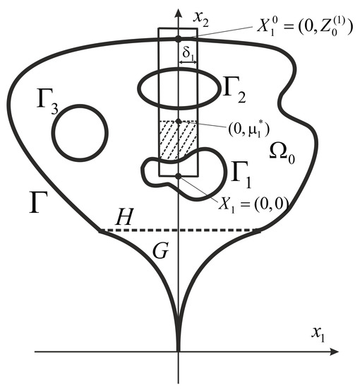
Figure 2. The strip ${\mathsf{{\rm Y}}}^{\left(1\right)}$ Dashed area is ${\widetilde{\mathsf{{\rm Y}}}}^{\left(1\right)}$.

In order to rewrite vector field ${\mathbf{b}}_j\left(z^{\left(j\right)}\right)$ in global coordinates let us take the orthogonal matrix $A_j$ with $det{A}_j=1$ such that $z^{\left(j\right)}=A_j(x-x_0.)$ Then it is easy to verify that

$${\mathbf{b}}_j^{\left(inn\right)}\left(x\right)=A_j^T{\mathbf{b}}_j\left(z^{\left(j\right)}\right){|}_{z^{\left(j\right)}=A_j(x-x_0)}.$$

Therefore, the flux carrier from the inner boundaries has the form:

$${\mathbf{b}}^{\left(inn\right)}\left(x\right)=\sum _{j=1}^N{\mathbf{b}}_j^{\left(inn\right)}\left(x\right).$$

Lemma 3.

The vector field ${\mathbf{b}}^{\left(inn\right)}$ is smooth and solenoidal. Moreover, $\mathrm{supp}{\mathbf{b}}^{\left(inn\right)}\subset {\mathsf{\Omega }}_0$,

$$\begin{array}{c}\underset{{\mathsf{\Gamma }}_j}{\int }{\mathbf{b}}^{\left(inn\right)}·\mathbf{n}dS=F_j,j=1,\dots ,N,\underset{\mathsf{\Gamma }\cap \partial {\mathsf{\Omega }}_0}{\int }{\mathbf{b}}^{\left(inn\right)}·\mathbf{n}dS=-{\displaystyle \sum _{j=1}^N}{F}_j\end{array}$$

(12)

and the following estimate

$$|{\mathbf{b}}^{\left(inn\right)}\left(x\right)|+|\nabla {\mathbf{b}}^{\left(inn\right)}\left(x\right)|\le c\sum _{j=1}^N\left|F_j\right|,\forall x\in {\overline{\mathsf{\Omega }}}_0$$

(13)

holds.

3.2. Flux Carrier from the Outer Boundary

The boundary condition $\mathbf{u}=\mathbf{a}$ is prescribed on $\left(\mathsf{\Gamma }\cap \partial {\mathsf{\Omega }}_0\right)\cup \left({\cup }_{j=1}^N{\mathsf{\Gamma }}_j\right).$ After subtracting the constructed flux carrier ${\mathbf{b}}^{\left(inn\right)}$, which “removes” the fluxes $F_j$ from the inner boundaries ${\mathsf{\Gamma }}_j,$$j=1,\dots ,N,$ we get a modified boundary value ${\mathbf{a}}_1=\mathbf{a}-{\mathbf{b}}^{\left(inn\right)}{|}_{\partial \mathsf{\Omega }}$ such that $\mathrm{supp}{\mathbf{a}}_1\subset \left(\mathsf{\Gamma }\cap \partial {\mathsf{\Omega }}_0\right)\cup \left({\cup }_{j=1}^N{\mathsf{\Gamma }}_j\right)$ and the flow rates of ${\mathbf{a}}_1$ over the inner boundaries ${\mathsf{\Gamma }}_j,j=1,\dots ,N,$ are equal to zero:

$$\begin{array}{c}\underset{{\mathsf{\Gamma }}_j}{\int }{\mathbf{a}}_1·\mathbf{n}dS=0,\end{array}$$

and the flow rate of ${\mathbf{a}}_1$ over the outer boundary $\mathsf{\Gamma }\cap \partial {\mathsf{\Omega }}_0$ is equal to $F_0+{\displaystyle \sum _{j=1}^N}{F}_j$:

$$\begin{array}{c}\underset{\mathsf{\Gamma }\cap \partial {\mathsf{\Omega }}_0}{\int }{\mathbf{a}}_1·\mathbf{n}dS=F_0+{\displaystyle \sum _{j=1}^N}{F}_j=\mathbb{F}.\end{array}$$

Now we remove the nonzero flux from the outer boundary $\mathsf{\Gamma }\cap \partial {\mathsf{\Omega }}_0$. For this we will need the notion of Stein’s regularised distance. Let $\mathcal{M}$ be a closed set in ${\mathbb{R}}^2.$ Stein’s regularised distance ${\mathsf{\Delta }}_{\mathcal{M}}\left(x\right)$ from the point x to the set $\mathcal{M}$ is an infinitely differentiable function in ${\mathbb{R}}^2\backslash \mathcal{M}$ and the following inequalities

$$a_1{d}_{\mathcal{M}}\left(x\right)\le {\mathsf{\Delta }}_{\mathcal{M}}\left(x\right)\le a_2{d}_{\mathcal{M}}\left(x\right),\left|{\mathrm{D}}^{\alpha }{\mathsf{\Delta }}_{\mathcal{M}}\left(x\right)\right|\le a_3{d}_{\mathcal{M}}^{1-\left|\alpha \right|}\left(x\right),$$

hold, where $d_{\mathcal{M}}\left(x\right)=dist(x,\mathcal{M})$ is the distance from x to $\mathcal{M}$. The positive constants $a_1,$$a_2$ and $a_3$ are independent of $\mathcal{M}$ (see [39], Chapter VI, Sections 1 and 2, 167–171, Theorem 2).

Let $\gamma$ be a smooth simple curve, which intersects the outer boundary at some point $x^{\left(out\right)}\in \mathsf{\Gamma }\cap \partial {\mathsf{\Omega }}_0,$ does not intersect or touch any inner boundary ${\mathsf{\Gamma }}_j,$$j=1,\dots ,N,$ and coincides with the straight line $x_1=0$ in G (see Figure 3).

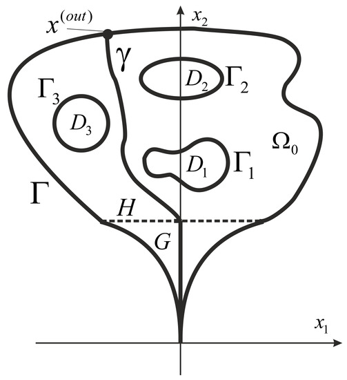
Figure 3. Curve $\gamma$.

Let us introduce a function

$$\xi \left(x\right)=\mathsf{\Psi }\left(ln{\displaystyle \frac{\rho \left({\mathsf{\Delta }}_{\gamma }\left(x\right)\right)}{{\mathsf{\Delta }}_{\partial \mathsf{\Omega }\backslash (\mathsf{\Gamma }\cap \partial {\mathsf{\Omega }}_0)}\left(x\right)}}\right),$$

where $\mathsf{\Psi }$ and $\rho$ are infinitely differentiable monotonic functions such that $\mathsf{\Psi }\left(t\right)=0$ for $t\le 0,$$\mathsf{\Psi }\left(t\right)=1$ for $t\ge 1,$ and $\rho \left(\tau \right)=\frac{a_1}{2}{d}_0$ for $\tau \le \frac{a_2}{2}$, $\rho \left(\tau \right)=\tau$ for $\tau \ge a_2{d}_0$, $d_0$ is the distance between the curve $\gamma$ and $\partial \mathsf{\Omega }\backslash (\mathsf{\Gamma }\cap \partial {\mathsf{\Omega }}_0)$. The functions ${\mathsf{\Delta }}_{\gamma }\left(x\right)$ and ${\mathsf{\Delta }}_{\partial \mathsf{\Omega }\backslash (\mathsf{\Gamma }\cap \partial {\mathsf{\Omega }}_0)}$ are regularised distances from x to $\gamma$ and $\partial \mathsf{\Omega }\backslash (\mathsf{\Gamma }\cap \partial {\mathsf{\Omega }}_0)$, respectively.

Lemma 4.

The function $\xi \left(x\right)$ vanishes at those points $x\in \overline{\mathsf{\Omega }}\backslash \left\{O\right\}$, where $\rho \left({\mathsf{\Delta }}_{\gamma }\left(x\right)\right)\le {\mathsf{\Delta }}_{\partial \mathsf{\Omega }\backslash (\mathsf{\Gamma }\cap \partial {\mathsf{\Omega }}_0)}\left(x\right)$, and $\xi \left(x\right)=1$ at points $x\in \overline{\mathsf{\Omega }}\backslash \left\{O\right\}$ where ${\mathsf{\Delta }}_{\partial \mathsf{\Omega }\backslash (\mathsf{\Gamma }\cap \partial {\mathsf{\Omega }}_0)}\left(x\right)\le e^{-1}\rho \left({\mathsf{\Delta }}_{\gamma }\left(x\right)\right)$. Moreover, the following inequalities

$$\left|\frac{\partial \xi \left(x\right)}{\partial x_k}\right|\le \frac{c}{{\mathsf{\Delta }}_{\partial \mathsf{\Omega }\backslash (\mathsf{\Gamma }\cap \partial {\mathsf{\Omega }}_0)}\left(x\right)}\le c_1,\left|\frac{{\partial }^2\xi \left(x\right)}{\partial x_k\partial x_l}\right|\le \frac{c}{{\mathsf{\Delta }}_{\partial \mathsf{\Omega }\backslash (\mathsf{\Gamma }\cap \partial {\mathsf{\Omega }}_0)}^2\left(x\right)}\le c_1,x\in {\overline{\mathsf{\Omega }}}_4,$$

(14)

hold with the constant $c_1$ dependent only on $a_1,a_2$ and $d_0$.

The proof of this lemma can be found in [40] (see Lemma 2).

Let us define a vector field

$${\mathbf{b}}^{\left(out\right)}\left(x\right)=-\mathbb{F}\left({\displaystyle \frac{\partial \tilde{\xi }\left(x\right)}{\partial x_2}},-{\displaystyle \frac{\partial \tilde{\xi }\left(x\right)}{\partial x_1}}\right),$$

where $\tilde{\xi }\left(x\right)$ coincides with $\xi \left(x\right)$ on the right side of the curve $\gamma$ and $\tilde{\xi }\left(x\right)=0$ on the left of $\gamma .$

By construction, the vector field ${\mathbf{b}}^{\left(out\right)}\left(x\right)$ is smooth, solenoidal and ${\mathbf{b}}^{\left(out\right)}\left(x\right){|}_{\partial \mathsf{\Omega }\backslash (\mathsf{\Gamma }\cap \partial {\mathsf{\Omega }}_0)}=0.$

Lemma 5.

There hold the relation

$$\begin{array}{c}\underset{\mathsf{\Gamma }\cap \partial {\mathsf{\Omega }}_4}{\int }{\mathbf{b}}^{\left(out\right)}·\mathbf{n}dS=\mathbb{F}\end{array}$$

(15)

and the estimate

$$|{\mathbf{b}}^{\left(out\right)}\left(x\right)|+|\nabla {\mathbf{b}}^{\left(out\right)}\left(x\right)|\le c|\mathbb{F}|\forall x\in {\overline{\mathsf{\Omega }}}_4.$$

(16)

Proof. 

Since $\mathrm{div}{\mathbf{b}}^{\left(out\right)}=0$, we have

$$\begin{array}{c}\underset{\mathsf{\Gamma }\cap \partial {\mathsf{\Omega }}_4}{\int }{\mathbf{b}}^{\left(out\right)}·\mathbf{n}dS=-\underset{\sigma \left(h_4\right)}{\int }{\mathbf{b}}^{\left(out\right)}·\mathbf{n}dS=\mathbb{F}\underset{-\phi \left(h_4\right)}{\overset{\phi \left(h_4\right)}{\int }}\left({\displaystyle \frac{\partial \tilde{\xi }\left(x\right)}{\partial x_2}},-{\displaystyle \frac{\partial \tilde{\xi }\left(x\right)}{\partial x_1}}\right)·(0,-1)dx\\ \\ =\mathbb{F}\underset{-\phi \left(h_4\right)}{\overset{\phi \left(h_4\right)}{\int }}{\displaystyle \frac{\partial \tilde{\xi }\left(x\right)}{\partial x_1}}d{x}_1=\mathbb{F}\left(\tilde{\xi }(\phi \left(h_4\right),h_4)-\tilde{\xi }(-\phi \left(h_4\right),h_4)\right)=\mathbb{F}.\end{array}$$

Estimate (16) follows from Lemma 4 and properties of the regularised distance. □

The modified boundary value ${\mathbf{a}}_2={\mathbf{a}}_1-{\mathbf{b}}^{\left(out\right)}{|}_{\partial \mathsf{\Omega }}$ has a support on $\left(\mathsf{\Gamma }\cap \partial {\mathsf{\Omega }}_0\right)\cup \left({\cup }_{j=1}^N{\mathsf{\Gamma }}_j\right)$ and the flow rates of ${\mathbf{a}}_2$ on $\mathsf{\Gamma }\cap \partial {\mathsf{\Omega }}_0$ and ${\mathsf{\Gamma }}_j,j=1,\dots ,N,$ are equal to zero:

$$\begin{array}{c}\underset{\mathsf{\Gamma }\cap \partial {\mathsf{\Omega }}_0}{\int }{\mathbf{a}}_2·\mathbf{n}dS=0,\underset{{\mathsf{\Gamma }}_j}{\int }{\mathbf{a}}_2·\mathbf{n}dS=0,j=1,\dots ,N.\end{array}$$

(17)

3.3. Extension of ${\mathbf{a}}_2$

The extension of the boundary value function having zero flux over the boundary was constructed by O.A. Ladyzhenskaya (see [37], Chapter V, Section 4, 127–128). To be more precise, in [37] was proved the following result

Lemma 6.

Let $D\subset {\mathbb{R}}^2$ be a bounded domain with Lipschitz boundary $\partial D$, $\mathcal{L}\subseteq \partial D$, $\mathrm{meas}\left(\mathcal{L}\right)>0$. Assume that the vector field $\mathbf{h}\in W^{1/2,2}(\partial D)$ satisfies the conditions $\underset{\mathcal{L}}{\int }\mathbf{h}·\mathbf{n}dS=0$, $\mathrm{supp}\mathbf{h}\subseteq \mathcal{L}$. Then $\mathbf{h}$ can be extended inside D in the form

$$\mathbf{H}(x,\epsilon )=\left(\frac{\partial \left(\chi \right(x,\epsilon \left)\mathbf{E}\right(x\left)\right)}{\partial x_2},-\frac{\partial \left(\chi \right(x,\epsilon \left)\mathbf{E}\right(x\left)\right)}{\partial x_1}\right),$$

(18)

where $\mathbf{E}\in W^{2,2}\left(D\right)$, $(\frac{\partial \mathbf{E}\left(x\right)}{\partial x_2},-\frac{\partial \mathbf{E}\left(x\right)}{\partial x_1}){|}_{\partial D}=\mathbf{h}$ and $\chi =\chi (x,\epsilon )$ is Hopf’s type cut-off function, i.e., χ is smooth, $\chi (x,\epsilon )=1$ on $\mathcal{L}$, $\mathrm{supp}\chi$ is contained in a small neighborhood of $\mathcal{L}$ and

$$|\nabla \chi (x,\epsilon )|\le \frac{\epsilon c}{\mathrm{dist}(x,\mathcal{L})}.$$

(19)

The constant c in (19) is independent of $\epsilon >0$.

The vector field $\mathbf{H}\in W^{1,2}\left(D\right)$ is solenoidal, $\mathbf{H}{|}_{\partial D}=\mathbf{h}$, $\mathrm{supp}\mathbf{H}$ is contained in a small neighbourhood of $\mathcal{L}$ and there holds the estimate

$${\parallel \mathbf{H}\parallel }_{W^{1,2}\left(D\right)}\le c\left(\epsilon \right){\parallel \mathbf{h}\parallel }_{W^{1/2,2}(\partial D)}.$$

(20)

Moreover, for any $\epsilon >0$ the vector field $\mathbf{H}$ satisfies the Leray-Hopf inequality

$$\begin{array}{c}\underset{D}{\int }\left(\mathbf{w}·\nabla \right)\mathbf{H}·\mathbf{w}dx\le c\epsilon \underset{D}{\int }{|\nabla \mathbf{w}|}^{2}dx\forall \mathbf{w}\in H\left(D\right)\end{array}$$

(21)

with the constant c independent of ε.

Because of the condition (17) we can apply Lemma 6 to ${\mathbf{a}}_2$ and we obtain the following result.

Lemma 7.

There exists a vector field ${\mathbf{b}}_0\in W^{1,2}\left(\mathsf{\Omega }\right)$ such that ${\mathbf{b}}_0{|}_{\partial \mathsf{\Omega }}={\mathbf{a}}_2$, $\mathrm{div}{\mathbf{b}}_0=0,$$\mathrm{supp}{\mathbf{b}}_0\subset {\overline{\mathsf{\Omega }}}_1$,

$$\parallel {\mathbf{b}}_0{\parallel }_{W^{1,2}\left(\mathsf{\Omega }\right)}\le c{\parallel {\mathbf{a}}_2\parallel }_{W^{1/2,2}(\partial \mathsf{\Omega })}.$$

(22)

Moreover,

$$\begin{array}{c}\underset{{\mathsf{\Omega }}_k}{\int }\left(\mathbf{w}·\nabla \right){\mathbf{b}}_0·\mathbf{w}dx\le c\epsilon \underset{{\mathsf{\Omega }}_k}{\int }{|\nabla \mathbf{w}|}^{2}dx\forall \mathbf{w}\in H\left({\mathsf{\Omega }}_k\right).\end{array}$$

(23)

The constant c in (23) is independent of $\epsilon >0$ and k.

3.4. Construction of Extension Coinciding with Asymptotic Decomposition near Cusp Point

Now we “glue” the above constructed vector field $\mathbf{B}={\mathbf{b}}_0+{\mathbf{b}}^{\left(inn\right)}+{\mathbf{b}}^{\left(out\right)}$ with the asymptotic decomposition ${\mathbf{U}}^{\left[J\right]}$.

Let $\zeta$ be a smooth cut-off function such that $\zeta \left(x_2\right)=1$ for $x_2\ge h_3$, $\zeta \left(x_2\right)=0$ for $x_2\le h_4$, $0\le \zeta \left(x_2\right)\le 1$. We put

$$\mathbf{A}={\mathbf{b}}_0+{\mathbf{b}}^{\left(inn\right)}+\zeta {\mathbf{b}}^{\left(out\right)}+\left(1-\zeta \right){\mathbf{U}}^{\left[J\right]}+{\mathbf{V}}^{\left[J\right]},$$

(24)

where ${\mathbf{V}}^{\left[J\right]}$ is the solution of the following problem

$$\begin{array}{cccc}\hfill \mathrm{div}{\mathbf{V}}^{\left[J\right]}& =-\nabla \zeta ·{\mathbf{b}}^{\left(out\right)}+\nabla \zeta ·{\mathbf{U}}^{\left[J\right]},\hfill & \hfill & x\in {\omega }_4,\hfill \\ \hfill {\mathbf{V}}^{\left[J\right]}& =0,\hfill & \hfill & x\in \partial {\omega }_4.\hfill \end{array}$$

(25)

Notice that $\underset{{\omega }_4}{\int }\left(\nabla \zeta ·{\mathbf{b}}^{\left(out\right)}-\nabla \zeta ·{\mathbf{U}}^{\left[J\right]}\right)dx=\underset{{\omega }_4}{\int }\mathrm{div}\left({\mathbf{b}}^{\left(out\right)}+\left(1-\zeta \right){\mathbf{U}}^{\left[J\right]}\right)dx=0$. Indeed,

$$\begin{array}{c}\underset{{\omega }_4}{\int }\mathrm{div}\left(\zeta {\mathbf{b}}^{\left(out\right)}+\left(1-\zeta \right){\mathbf{U}}^{\left[J\right]}\right)dx=\underset{\partial {\omega }_4}{\int }\zeta {\mathbf{b}}^{\left(out\right)}·\mathbf{n}dS+\underset{\partial {\omega }_4}{\int }\left(1-\zeta \right){\mathbf{U}}^{\left[J\right]}·\mathbf{n}dS\hfill \\ =\underset{\sigma \left(h_3\right)}{\int }{\mathbf{b}}^{\left(out\right)}·\mathbf{n}dS-\underset{\sigma \left(h_4\right)}{\int }{\mathbf{U}}^{\left[J\right]}·\mathbf{n}dS=\left(F_0+{\displaystyle \sum _{j=1}^N}{F}_j\right)-{\displaystyle \underset{-\phi \left(h_4\right)}{\overset{\phi \left(h_4\right)}{\int }}}{U}_2^{\left[J\right]}d{x}_1=0,\hfill \end{array}$$

where we used the fact that ${\mathbf{b}}^{\left(inn\right)}=0$ in ${\omega }_4.$ Therefore, there exists a solution ${\mathbf{V}}^{\left[J\right]}\in {\mathring{W}}^{1,2}\left({\omega }_4\right)$ of problem (25) satisfying the estimate

$$\parallel \nabla {\mathbf{V}}^{\left[J\right]}{\parallel }_{L^2\left({\omega }_4\right)}\le c\parallel \nabla \zeta ·\left({\mathbf{b}}^{\left(out\right)}+{\mathbf{U}}^{\left[J\right]}\right){\parallel }_{L^2\left({\omega }_2\right)}\le c\left|\mathbb{F}\right|,$$

(26)

see [41].

Since $\mathrm{div}\left({\mathbf{b}}_0+{\mathbf{b}}^{\left(inn\right)}\right)=0$ and $\mathrm{supp}\left({\mathbf{b}}_0+{\mathbf{b}}^{\left(inn\right)}\right)\subset {\overline{\mathsf{\Omega }}}_4$, from the construction we conclude the following result.

Lemma 8.

The vector field $\mathbf{A}\in W_{loc}^{1,2}(\overline{\mathsf{\Omega }}\backslash \left\{O\right\})$ satisfies the boundary condition $\mathbf{A}{|}_{\partial \mathsf{\Omega }}=\mathbf{a}$, $\mathbf{A}$ is solenoidal and $\mathbf{A}\left(x\right)={\mathbf{U}}^{\left[J\right]}\left(x\right)$ for $x_2\le h_4$.

4. Existence and Uniqueness of Weak Solution

In this section we prove the existence of the weak solution of problem (1).

First assume that $\left(\mathbf{u},p\right)$ is a classical solution of (1). Multiplying (1)₁ by the test function $\mathbf{\eta }\in C_0^{\infty }\left(\mathsf{\Omega }\right)$ and integrating by parts, we obtain

$$\begin{array}{c}\nu \underset{\mathsf{\Omega }}{\int }\nabla \mathbf{u}·\nabla \mathbf{\eta }dx+\underset{\mathsf{\Omega }}{\int }\left(\mathbf{u}·\nabla \right)\mathbf{u}·\mathbf{\eta }dx-\underset{\mathsf{\Omega }}{\int }p\mathrm{div}\mathbf{\eta }dx=\underset{\mathsf{\Omega }}{\int }\mathbf{f}·\mathbf{\eta }dx\forall \mathbf{\eta }\in C_0^{\infty }\left(\mathsf{\Omega }\right).\end{array}$$

(27)

We look for the solution $\left(\mathbf{u},p\right)$ in the form

$$\mathbf{u}=\mathbf{A}+\mathbf{v},p=(1-\zeta )P^{\left[j\right]}+\tilde{p},$$

(28)

where $\mathbf{A}$ is the extension of the boundary value $\mathbf{a}$ constructed in the previous section, $P^{\left[j\right]}$ is defined by (6)₃ and $\mathbf{v}\in H\left(\mathsf{\Omega }\right)$. Substituting (28) into (27) we obtain

$$\begin{array}{c}\nu \underset{\mathsf{\Omega }}{\int }\nabla \mathbf{v}·\nabla \mathbf{\eta }dx+\underset{\mathsf{\Omega }}{\int }\left((\mathbf{v}+\mathbf{A})·\nabla \right)\mathbf{v}·\mathbf{\eta }dx+\underset{\mathsf{\Omega }}{\int }\left(\mathbf{v}·\nabla \right)\mathbf{A}·\mathbf{\eta }dx={⟨\widehat{\mathbf{f}},\mathbf{\eta }⟩}_{\mathsf{\Omega }}\forall \mathbf{\eta }\in J_0^{\infty }\left(\mathsf{\Omega }\right),\end{array}$$

(29)

where

$$\begin{array}{c}{⟨\widehat{\mathbf{f}},\mathbf{\eta }⟩}_{\mathsf{\Omega }}=\underset{\mathsf{\Omega }}{\int }\mathbf{f}·\mathbf{\eta }dx-\nu \underset{\mathsf{\Omega }}{\int }\nabla \mathbf{A}·\nabla \mathbf{\eta }dx-\underset{\mathsf{\Omega }}{\int }\left(\mathbf{A}·\nabla \right)\mathbf{A}·\mathbf{\eta }dx-\underset{\mathsf{\Omega }}{\int }\nabla \left((1-\zeta )P^{\left[J\right]}\right)·\mathbf{\eta }dx.\end{array}$$

(30)

The vector field $\mathbf{v}$ will be found as a limit of the sequence $\left\{{\mathbf{v}}_k\right\}$, where ${\mathbf{v}}_k$ are weak solutions in the domains ${\mathsf{\Omega }}_k$, that is, the vector fields ${\mathbf{v}}_k\in H\left({\mathsf{\Omega }}_k\right),$ satisfy the integral identities

$$\begin{array}{c}\nu \underset{{\mathsf{\Omega }}_k}{\int }\nabla {\mathbf{v}}_k·\nabla \mathbf{\eta }dx+\underset{{\mathsf{\Omega }}_k}{\int }\left(({\mathbf{v}}_k+\mathbf{A})·\nabla \right){\mathbf{v}}_k·\mathbf{\eta }dx+\underset{{\mathsf{\Omega }}_k}{\int }\left({\mathbf{v}}_k·\nabla \right)\mathbf{A}·\mathbf{\eta }dx={⟨\widehat{\mathbf{f}},\mathbf{\eta }⟩}_{{\mathsf{\Omega }}_k}\forall \mathbf{\eta }\in H\left({\mathsf{\Omega }}_k\right).\end{array}$$

(31)

Theorem 1.

Let $\mathbf{f}\in L^2\left(\mathsf{\Omega }\right)$, $\mathbf{a}\in W^{1/2,2}(\partial \mathsf{\Omega })$ and $\mathrm{supp}\mathbf{a}\subset \left(\mathsf{\Gamma }\cap \partial {\mathsf{\Omega }}_0\right)\cup \left({\cup }_{j=1}^N{\mathsf{\Gamma }}_j\right)$. There exists a number ${\mathcal{F}}_0>0$ such that if

$${\displaystyle \sum _{j=0}^N}\left|F_j\right|\le {\mathcal{F}}_0,$$

(32)

then problem (31) admits at least one solution ${\mathbf{v}}_k\in H\left({\mathsf{\Omega }}_k\right)$. There holds the estimate

$$\parallel \nabla {\mathbf{v}}_k{\parallel }_{L^2\left(\mathsf{\Omega }\right)}^2\le c\left({\parallel \mathbf{f}\parallel }_{L^2\left({\mathsf{\Omega }}_k\right)}^2+{\parallel \mathbf{a}\parallel }_{W^{1/2,2}(\partial \mathsf{\Omega })}^2+{\parallel \mathbf{a}\parallel }_{W^{1/2,2}(\partial \mathsf{\Omega })}^4\right)$$

(33)

with the constant c independent of k.

Proof. 

It is well known (see [37]) that integral identity (31) is equivalent to the operator equation

$${\mathbf{v}}_k=\mathcal{B}{\mathbf{v}}_k$$

(34)

with a completely continuous operator $\mathcal{B}:H\left({\mathsf{\Omega }}_k\right)\hookrightarrow H\left({\mathsf{\Omega }}_k\right)$, defined by the relation

$$\begin{array}{c}{[\mathcal{B}{\mathbf{v}}_k,\mathbf{\eta }]}_{{\mathsf{\Omega }}_k}=-{\nu }^{-1}\underset{{\mathsf{\Omega }}_k}{\int }\left(({\mathbf{v}}_k+\mathbf{A})·\nabla \right){\mathbf{v}}_k·\mathbf{\eta }dx-{\nu }^{-1}\underset{{\mathsf{\Omega }}_k}{\int }\left({\mathbf{v}}_k·\nabla \right)\mathbf{A}·\mathbf{\eta }dx+{\nu }^{-1}{⟨\widehat{\mathbf{f}},\mathbf{\eta }⟩}_{{\mathsf{\Omega }}_k},\end{array}$$

where ${[\mathbf{w},\mathbf{\eta }]}_{{\mathsf{\Omega }}_k}=\underset{{\mathsf{\Omega }}_k}{\int }\nabla \mathbf{w}·\nabla \mathbf{\eta }dx$ is the scalar product in $H\left({\mathsf{\Omega }}_k\right)$.

So, the solvability of Equation (34) will follow from the Leray–Schauder theorem provided we prove that the norms of all possible solutions of the operator equations

$${\mathbf{v}}_k^{\left(\lambda \right)}=\lambda \mathcal{B}{\mathbf{v}}_k^{\left(\lambda \right)},\lambda \in [0;1],$$

(35)

are bounded by a constant independent of $\lambda$.

Operator Equation (35) is equivalent to the identity

$$\begin{array}{c}\nu \underset{{\mathsf{\Omega }}_k}{\int }\nabla {\mathbf{v}}_k^{\left(\lambda \right)}·\nabla \mathbf{\eta }dx+\lambda \underset{{\mathsf{\Omega }}_k}{\int }\left(({\mathbf{v}}_k^{\left(\lambda \right)}+\mathbf{A})·\nabla \right){\mathbf{v}}_k^{\left(\lambda \right)}·\mathbf{\eta }dx+\lambda \underset{{\mathsf{\Omega }}_k}{\int }\left({\mathbf{v}}_k^{\left(\lambda \right)}·\nabla \right)\mathbf{A}·\mathbf{\eta }dx\\ =\lambda {⟨\widehat{\mathbf{f}},\mathbf{\eta }⟩}_{{\mathsf{\Omega }}_k}\forall \mathbf{\eta }\in H\left({\mathsf{\Omega }}_k\right).\end{array}$$

(36)

Taking in (36) $\mathbf{\eta }={\mathbf{v}}_k^{\left(\lambda \right)}$ we obtain

$$\begin{array}{c}\nu \underset{{\mathsf{\Omega }}_k}{\int }{|\nabla {\mathbf{v}}_k^{\left(\lambda \right)}|}^{2}dx=-\lambda \underset{{\mathsf{\Omega }}_k}{\int }\left({\mathbf{v}}_k^{\left(\lambda \right)}·\nabla \right)\mathbf{A}·{\mathbf{v}}_k^{\left(\lambda \right)}dx+\lambda {⟨\widehat{\mathbf{f}},{\mathbf{v}}_k^{\left(\lambda \right)}⟩}_{{\mathsf{\Omega }}_k}.\end{array}$$

(37)

To estimate the term $\lambda {⟨\widehat{\mathbf{f}},{\mathbf{v}}_k^{\left(\lambda \right)}⟩}_{{\mathsf{\Omega }}_k}$ in the right hand side of (37), we use the representation (24) for the vector field $\mathbf{A}$. We denote ${\mathbf{A}}_1={\mathbf{b}}_0+{\mathbf{b}}^{\left(inn\right)}+\zeta {\mathbf{b}}^{\left(out\right)}+{\mathbf{V}}^{\left[J\right]}$ and ${\mathbf{A}}_2=(1-\zeta ){\mathbf{U}}^{\left[J\right]}$, so that $\mathbf{A}={\mathbf{A}}_1+{\mathbf{A}}_2$. Since $\mathrm{supp}{\mathbf{A}}_1\subset {\mathsf{\Omega }}_4$, using estimates (13), (16), (22) and (26), the embedding $W^{1,2}\left({\mathsf{\Omega }}_4\right)\hookrightarrow L^4\left({\mathsf{\Omega }}_4\right)$ and the definition of ${\mathbf{a}}_2=\mathbf{a}-\left({\mathbf{b}}^{\left(inn\right)}+{\mathbf{b}}^{\left(out\right)}\right){|}_{\partial \mathsf{\Omega }}$, we obtain the following inequality

$$\begin{array}{c}\lambda \nu |\underset{{\mathsf{\Omega }}_4}{\int }\nabla {\mathbf{A}}_1·\nabla {\mathbf{v}}_k^{\left(\lambda \right)}dx|+\lambda |\underset{{\mathsf{\Omega }}_4}{\int }\left({\mathbf{A}}_1·\nabla \right){\mathbf{v}}_k^{\left(\lambda \right)}·{\mathbf{A}}_{1}dx|\\ \le c\left(\parallel \nabla {\mathbf{A}}_1{\parallel }_{L^2\left({\mathsf{\Omega }}_k\right)}^2+{\parallel {\mathbf{A}}_1\parallel }_{L^4\left({\mathsf{\Omega }}_k\right)}^4\right)+\epsilon {\parallel \nabla {\mathbf{v}}_k^{\left(\lambda \right)}\parallel }_{L^2\left({\mathsf{\Omega }}_k\right)}^2\\ \le c\left[{\left({\displaystyle \sum _{j=0}^N}\left|F_j\right|\right)}^2+{\left({\displaystyle \sum _{j=0}^N}\left|F_j\right|\right)}^4+{\parallel \mathbf{a}\parallel }_{W^{1/2,2}(\partial \mathsf{\Omega })}^2+{\parallel \mathbf{a}\parallel }_{W^{1/2,2}(\partial \mathsf{\Omega })}^4\right]+\epsilon {\parallel \nabla {\mathbf{v}}_k^{\left(\lambda \right)}\parallel }_{L^2\left({\mathsf{\Omega }}_k\right)}^2\\ \le c\left[{\parallel \mathbf{a}\parallel }_{W^{1/2,2}(\partial \mathsf{\Omega })}^2+{\parallel \mathbf{a}\parallel }_{W^{1/2,2}(\partial \mathsf{\Omega })}^4\right]+\epsilon {\parallel \nabla {\mathbf{v}}_k^{\left(\lambda \right)}\parallel }_{L^2\left({\mathsf{\Omega }}_k\right)}^2.\end{array}$$

(38)

Since $\mathrm{supp}({\mathbf{b}}_0+{\mathbf{b}}^{\left(inn\right)})\subset {\mathsf{\Omega }}_3$, we have $\left(({\mathbf{b}}_0+{\mathbf{b}}^{\left(inn\right)})·\nabla \right){\mathbf{A}}_2+\left({\mathbf{A}}_2·\nabla \right)({\mathbf{b}}_0+{\mathbf{b}}^{\left(inn\right)})=0$. Thus, by (7), (16) and (26),

$$\begin{array}{c}\lambda |\underset{{\mathsf{\Omega }}_4}{\int }\left({\mathbf{A}}_1·\nabla \right){\mathbf{v}}_k^{\left(\lambda \right)}·{\mathbf{A}}_{2}dx|+\lambda |\underset{{\mathsf{\Omega }}_4}{\int }\left({\mathbf{A}}_2·\nabla \right){\mathbf{v}}_k^{\left(\lambda \right)}·{\mathbf{A}}_{1}dx|\\ \le |\underset{{\omega }_4}{\int }\left(({\mathbf{V}}^{\left[J\right]}+{\mathbf{b}}^{\left(out\right)})·\nabla \right){\mathbf{v}}_k^{\left(\lambda \right)}·{\mathbf{U}}^{\left[J\right]}dx|+|\underset{{\omega }_4}{\int }\left({\mathbf{U}}^{\left[J\right]}·\nabla \right){\mathbf{v}}_k^{\left(\lambda \right)}·({\mathbf{V}}^{\left[J\right]}+{\mathbf{b}}^{\left(out\right)})dx|\\ \le c\left(\parallel {\mathbf{V}}^{\left[J\right]}{\parallel }_{L^4\left({\omega }_4\right)}^4+\parallel {\mathbf{b}}^{\left(out\right)}{\parallel }_{L^4\left({\omega }_4\right)}^4+{\parallel {\mathbf{U}}^{\left[J\right]}\parallel }_{L^4\left({\omega }_4\right)}^4\right)+\epsilon {\parallel \nabla {\mathbf{v}}_k^{\left(\lambda \right)}\parallel }_{L^2\left({\mathsf{\Omega }}_k\right)}^2\\ \le c\left(\parallel {\mathbf{V}}^{\left[J\right]}{\parallel }_{W^{1,2}\left({\omega }_4\right)}^4+{\left|\mathbb{F}\right|}^4\right)+\epsilon \parallel \nabla {\mathbf{v}}_k^{\left(\lambda \right)}{\parallel }_{L^2\left({\mathsf{\Omega }}_k\right)}^2\le c{\left({\displaystyle \sum _{j=0}^N}\left|F_j\right|\right)}^4+\epsilon {\parallel \nabla {\mathbf{v}}_k^{\left(\lambda \right)}\parallel }_{L^2\left({\mathsf{\Omega }}_k\right)}^2\\ \le {c\parallel \mathbf{a}\parallel }_{W^{1/2,2}(\partial \mathsf{\Omega })}^4+\epsilon {\parallel \nabla {\mathbf{v}}_k^{\left(\lambda \right)}\parallel }_{L^2\left({\mathsf{\Omega }}_k\right)}^2.\end{array}$$

(39)

Further, the straightforward calculations give the equality

$$\begin{array}{c}\lambda \nu \underset{{\mathsf{\Omega }}_k\backslash {\mathsf{\Omega }}_3}{\int }\nabla {\mathbf{A}}_2·\nabla {\mathbf{v}}_k^{\left(\lambda \right)}dx+\lambda \underset{{\mathsf{\Omega }}_k\backslash {\mathsf{\Omega }}_3}{\int }\left({\mathbf{A}}_2·\nabla \right){\mathbf{A}}_2·{\mathbf{v}}_k^{\left(\lambda \right)}dx+\lambda \underset{{\mathsf{\Omega }}_k\backslash {\mathsf{\Omega }}_3}{\int }\nabla \left((1-\zeta )P^{\left[J\right]}\right)·{\mathbf{v}}_k^{\left(\lambda \right)}dx\\ =\lambda \nu \underset{{\mathsf{\Omega }}_k\backslash {\mathsf{\Omega }}_3}{\int }\nabla \left((1-\zeta ){\mathbf{U}}^{\left[J\right]}\right)·\nabla {\mathbf{v}}_k^{\left(\lambda \right)}dx+\lambda \underset{{\mathsf{\Omega }}_k\backslash {\mathsf{\Omega }}_3}{\int }\left((1-\zeta ){\mathbf{U}}^{\left[J\right]}·\nabla \right)\left((1-\zeta ){\mathbf{U}}^{\left[J\right]}\right)·{\mathbf{v}}_k^{\left(\lambda \right)}dx\\ +\lambda \underset{{\mathsf{\Omega }}_k\backslash {\mathsf{\Omega }}_3}{\int }\nabla \left((1-\zeta )P^{\left[J\right]}\right)·{\mathbf{v}}_k^{\left(\lambda \right)}dx\\ =\lambda \underset{{\mathsf{\Omega }}_k\backslash {\mathsf{\Omega }}_4}{\int }\left(-\nu \mathsf{\Delta }{\mathbf{U}}^{\left[J\right]}+({\mathbf{U}}^{\left[J\right]}·\nabla \right){\mathbf{U}}^{\left[J\right]}+\nabla P^{\left[J\right]})·{\mathbf{v}}_k^{\left(\lambda \right)}dx\\ +\lambda \nu \underset{{\omega }_3}{\int }\left(-(1-\zeta )\mathsf{\Delta }{\mathbf{U}}^{\left[J\right]}+2\nabla \zeta ·\nabla {\mathbf{U}}^{\left[J\right]}+{\zeta }^{″}{\mathbf{U}}^{\left[J\right]}\right)·{\mathbf{v}}_k^{\left(\lambda \right)}dx\\ +\lambda \underset{{\omega }_3}{\int }\left(-P^{\left[J\right]}\nabla \zeta +(1-\zeta )\nabla P^{\left[J\right]}\right)·{\mathbf{v}}_k^{\left(\lambda \right)}dx\\ +\lambda \underset{{\omega }_3}{\int }\left({(1-\zeta )}^2\left({\mathbf{U}}^{\left[J\right]}·\nabla \right){\mathbf{U}}^{\left[J\right]}·{\mathbf{v}}_k^{\left(\lambda \right)}-(1-\zeta )\left({\mathbf{U}}^{\left[J\right]}·\nabla \right)\zeta \left({\mathbf{U}}^{\left[J\right]}·{\mathbf{v}}_k^{\left(\lambda \right)}\right)\right)dx=\lambda {\displaystyle \sum _{k=1}^4}{J}_k.\end{array}$$

Because the asymptotic decomposition $({\mathbf{U}}^{\left[J\right]},P^{\left[J\right]})$ satisfies Equation (8), by (9), we obtain

$$\begin{array}{c}\lambda J_1=\lambda \underset{{\mathsf{\Omega }}_k\backslash {\mathsf{\Omega }}_4}{\int }\left(-\nu \mathsf{\Delta }{\mathbf{U}}^{\left[J\right]}+({\mathbf{U}}^{\left[J\right]}·\nabla \right){\mathbf{U}}^{\left[J\right]}+\nabla P^{\left[J\right]})·{\mathbf{v}}_k^{\left(\lambda \right)}dx=\lambda \underset{{\mathsf{\Omega }}_k\backslash {\mathsf{\Omega }}_4}{\int }{\mathbf{H}}^{\left[J\right]}·{\mathbf{v}}_k^{\left(\lambda \right)}dx\\ \le c\underset{{\mathsf{\Omega }}_k\backslash {\mathsf{\Omega }}_4}{\int }|{\mathbf{H}}^{\left[J\right]}{|}^{2}dx+\epsilon \parallel \nabla {\mathbf{v}}_k^{\left(\lambda \right)}{\parallel }_{L^2\left({\mathsf{\Omega }}_k\right)}^2\le c\left({\left|\mathbb{F}\right|}^2+{\left|\mathbb{F}\right|}^4\right)+\epsilon {\parallel \nabla {\mathbf{v}}_k^{\left(\lambda \right)}\parallel }_{L^2\left({\mathsf{\Omega }}_k\right)}^2\\ \le c\left({\parallel \mathbf{a}\parallel }_{W^{1/2,2}(\partial \mathsf{\Omega })}^2+{\parallel \mathbf{a}\parallel }_{W^{1/2,2}(\partial \mathsf{\Omega })}^4\right)+\epsilon {\parallel \nabla {\mathbf{v}}_k^{\left(\lambda \right)}\parallel }_{L^2\left({\mathsf{\Omega }}_k\right)}^2.\end{array}$$

(40)

The integrals $J_k$, $k=2,3,4,$ can be estimated using (7), and we get

$$\begin{array}{c}\lambda \left(|J_2|+|J_3|+|J_4\right)\le c\left({\parallel \mathbf{a}\parallel }_{W^{1/2,2}(\partial \mathsf{\Omega })}^2+{\parallel \mathbf{a}\parallel }_{W^{1/2,2}(\partial \mathsf{\Omega })}^4\right)+\epsilon {\parallel \nabla {\mathbf{v}}_k^{\left(\lambda \right)}\parallel }_{L^2\left({\mathsf{\Omega }}_k\right)}^2.\end{array}$$

(41)

From (39)–(41) it follows that

$$\begin{array}{c}\left|\lambda {⟨\widehat{\mathbf{f}},{\mathbf{v}}_k^{\left(\lambda \right)}⟩}_{{\mathsf{\Omega }}_k}\right|\le c\left({\parallel \mathbf{f}\parallel }_{L^2\left({\mathsf{\Omega }}_k\right)}^2+{\parallel \mathbf{a}\parallel }_{W^{1/2,2}(\partial \mathsf{\Omega })}^2+{\parallel \mathbf{a}\parallel }_{W^{1/2,2}(\partial \mathsf{\Omega })}^4\right)+c\epsilon {\parallel \nabla {\mathbf{v}}_k^{\left(\lambda \right)}\parallel }_{L^2\left({\mathsf{\Omega }}_k\right)}^2.\end{array}$$

Substituting this estimate into (37) and choosing $\epsilon$ sufficiently small we obtain

$$\begin{array}{c}\frac{\nu }{2}\underset{{\mathsf{\Omega }}_k}{\int }{|\nabla {\mathbf{v}}_k^{\left(\lambda \right)}|}^{2}dx\le -\lambda \underset{{\mathsf{\Omega }}_k}{\int }\left({\mathbf{v}}_k^{\left(\lambda \right)}·\nabla \right)\mathbf{A}·{\mathbf{v}}_k^{\left(\lambda \right)}dx+c\left({\parallel \mathbf{f}\parallel }_{L^2\left({\mathsf{\Omega }}_k\right)}^2+{\parallel \mathbf{a}\parallel }_{W^{1/2,2}(\partial \mathsf{\Omega })}^2+{\parallel \mathbf{a}\parallel }_{W^{1/2,2}(\partial \mathsf{\Omega })}^4\right).\end{array}$$

(42)

The constant c in (42) is independent of k.

Consider now the integral $\lambda \underset{{\mathsf{\Omega }}_k}{\int }\left({\mathbf{v}}_k^{\left(\lambda \right)}·\nabla \right)\mathbf{A}·{\mathbf{v}}_k^{\left(\lambda \right)}dx=-\lambda \underset{{\mathsf{\Omega }}_k}{\int }\left({\mathbf{v}}_k^{\left(\lambda \right)}·\nabla \right){\mathbf{v}}_k^{\left(\lambda \right)}·\mathbf{A}dx$. In virtue of Lemmas 3 and 5, we have

$$\begin{array}{c}\lambda |\underset{{\mathsf{\Omega }}_k}{\int }\left({\mathbf{v}}_k^{\left(\lambda \right)}·\nabla \right){\mathbf{v}}_k^{\left(\lambda \right)}·\left({\mathbf{b}}^{\left(inn\right)}+\zeta {\mathbf{b}}^{\left(out\right)}\right)dx|\\ \le \parallel {\mathbf{v}}_k^{\left(\lambda \right)}{\parallel }_{L^4\left({\mathsf{\Omega }}_k\right)}{\parallel \nabla {\mathbf{v}}_k^{\left(\lambda \right)}\parallel }_{L^2\left({\mathsf{\Omega }}_k\right)}\left(\parallel {\mathbf{b}}^{\left(inn\right)}{\parallel }_{L^4\left({\mathsf{\Omega }}_4\right)}+{\parallel {\mathbf{b}}^{\left(out\right)}\parallel }_{L^4\left({\mathsf{\Omega }}_4\right)}\right)\\ \le c{\displaystyle \sum _{i=0}^N}|F_i|\parallel \nabla {\mathbf{v}}_k^{\left(\lambda \right)}{\parallel }_{L^2\left({\mathsf{\Omega }}_k\right)}^2.\end{array}$$

(43)

By (26),

$$\begin{array}{c}\lambda |\underset{{\mathsf{\Omega }}_k}{\int }\left({\mathbf{v}}_k^{\left(\lambda \right)}·\nabla \right){\mathbf{V}}^{\left[J\right]}·{\mathbf{v}}_k^{\left(\lambda \right)}dx|\le \parallel {\mathbf{v}}_k^{\left(\lambda \right)}{\parallel }_{L^4\left({\mathsf{\Omega }}_k\right)}^2\parallel \nabla {\mathbf{V}}^{\left[J\right]}{\parallel }_{L^2\left({\omega }_4\right)}\le c{\displaystyle \sum _{i=0}^N}|F_i|\parallel \nabla {\mathbf{v}}_k^{\left(\lambda \right)}{\parallel }_{L^2\left({\mathsf{\Omega }}_k\right)}^2.\end{array}$$

(44)

For the integral $\lambda \underset{{\mathsf{\Omega }}_k}{\int }\left({\mathbf{v}}_k^{\left(\lambda \right)}·\nabla \right){\mathbf{v}}_k^{\left(\lambda \right)}·{\mathbf{U}}^{\left(\right[J]}(1-\zeta )dx$ inequalities (7) and (5) yield

$$\begin{array}{c}\lambda |\underset{{\mathsf{\Omega }}_k\backslash {\mathsf{\Omega }}_3}{\int }\left({\mathbf{v}}_k^{\left(\lambda \right)}·\nabla \right){\mathbf{v}}_k^{\left(\lambda \right)}·{\mathbf{U}}^{\left(\right[J]}(1-\zeta )dx|\le {\left(\underset{{\mathsf{\Omega }}_k\backslash {\mathsf{\Omega }}_3}{\int }|{\mathbf{v}}_k^{\left(\lambda \right)}{|}^2{\left|{\mathbf{U}}^{\left(\right[J]}\right|}^{2}dx\right)}^{1/2}{\parallel \nabla {\mathbf{v}}_k^{\left(\lambda \right)}\parallel }_{L^2\left({\mathsf{\Omega }}_k\right)}\\ \le c\left|\mathbb{F}\right|{\left(\underset{h_k}{\overset{h_3}{\int }}\underset{-\phi \left(x_2\right)}{\overset{\phi \left(x_2\right)}{\int }}{\displaystyle \frac{|{\mathbf{v}}_k^{\left(\lambda \right)}{|}^2}{{\phi }^2\left(x_2\right)}}d{x}_{1}d{x}_2\right)}^{1/2}\parallel \nabla {\mathbf{v}}_k^{\left(\lambda \right)}{\parallel }_{L^2\left({\mathsf{\Omega }}_k\right)}\le c{\displaystyle \sum _{i=0}^N}|F_i|\parallel \nabla {\mathbf{v}}_k^{\left(\lambda \right)}{\parallel }_{L^2\left({\mathsf{\Omega }}_k\right)}^2.\end{array}$$

(45)

Finally, using Leray–Hopf’s inequality (23), we estimate the integral $\underset{{\mathsf{\Omega }}_k}{\int }\left({\mathbf{v}}_k^{\left(\lambda \right)}·\nabla \right){\mathbf{b}}_0·{\mathbf{v}}_k^{\left(\lambda \right)}dx$:

$$\begin{array}{c}\underset{{\mathsf{\Omega }}_k}{\int }\left({\mathbf{v}}_k^{\left(\lambda \right)}·\nabla \right){\mathbf{b}}_0·{\mathbf{v}}_k^{\left(\lambda \right)}dx\le c_0\epsilon \underset{{\mathsf{\Omega }}_k}{\int }{|\nabla {\mathbf{v}}_k^{\left(\lambda \right)}|}^{2}dx.\end{array}$$

(46)

Estimates (43)–(46) yield the inequality

$$\begin{array}{c}\lambda \underset{{\mathsf{\Omega }}_k}{\int }\left({\mathbf{v}}_k^{\left(\lambda \right)}·\nabla \right)\mathbf{A}·{\mathbf{v}}_k^{\left(\lambda \right)}dx\le \left(c_0\epsilon +c_{*}{\displaystyle \sum _{i=0}^N}\left|F_i\right|\right)\underset{{\mathsf{\Omega }}_k}{\int }{|\nabla {\mathbf{v}}_k^{\left(\lambda \right)}|}^{2}dx\forall \lambda \in [0,1],\end{array}$$

(47)

where the constants $c_0$ and $c_{*}$ are independent of k and $\lambda$. Thus, estimate (42) takes the form

$$\begin{array}{c}\frac{\nu }{2}\underset{{\mathsf{\Omega }}_k}{\int }|\nabla {\mathbf{v}}_k^{\left(\lambda \right)}{|}^{2}dx\le \left(c_0\epsilon +c_{*}{\mathcal{F}}_0\right)\underset{{\mathsf{\Omega }}_k}{\int }{|\nabla {\mathbf{v}}_k^{\left(\lambda \right)}|}^{2}dx+c\left({\parallel \mathbf{f}\parallel }_{L^2\left(\mathsf{\Omega }\right)}^2+{\parallel \mathbf{a}\parallel }_{W^{1/2,2}(\partial \mathsf{\Omega })}^2+{\parallel \mathbf{a}\parallel }_{W^{1/2,2}(\partial \mathsf{\Omega })}^4\right).\end{array}$$

Choosing $\epsilon$ sufficiently small, say $\epsilon =\frac{\nu }{8c_0}$ and assuming that ${\mathcal{F}}_0=\frac{\nu }{8c_{*}}$ from the last inequality we derive

$$\begin{array}{c}\frac{\nu }{2}\underset{{\mathsf{\Omega }}_k}{\int }{|\nabla {\mathbf{v}}_k^{\left(\lambda \right)}|}^{2}dx\le c\left({\parallel \mathbf{f}\parallel }_{L^2\left(\mathsf{\Omega }\right)}^2+{\parallel \mathbf{a}\parallel }_{W^{1/2,2}(\partial \mathsf{\Omega })}^2+{\parallel \mathbf{a}\parallel }_{W^{1/2,2}(\partial \mathsf{\Omega })}^4\right).\end{array}$$

So, the norms $\parallel \nabla {\mathbf{v}}_k^{\left(\lambda \right)}{\parallel }_{L^2\left({\mathsf{\Omega }}_k\right)}^2$ of all possible solutions ${\mathbf{v}}_k^{\left(\lambda \right)}$ of operator Equation (35) are bounded by a constant independent of $\lambda \in [0,1]$ and, according to the Leray–Schauder theorem, operator Equation (34) has at least one solution ${\mathbf{v}}_k\in H\left({\mathsf{\Omega }}_k\right)$. Moreover, for ${\mathbf{v}}_k$ holds estimate (33). □

Theorem 2.

Suppose that the conditions of Theorem 1 are fulfilled. Then problem (29) admits a solution $\mathbf{v}\in H\left(\mathsf{\Omega }\right)$ satisfying the following estimate

$${\parallel \nabla \mathbf{v}\parallel }_{L^2\left(\mathsf{\Omega }\right)}^2\le c\left({\parallel \mathbf{f}\parallel }_{L^2\left(\mathsf{\Omega }\right)}^2+{\parallel \mathbf{a}\parallel }_{W^{1/2,2}(\partial \mathsf{\Omega })}^2+{\parallel \mathbf{a}\parallel }_{W^{1/2,2}(\partial \mathsf{\Omega })}^4\right).$$

(48)

Proof. 

Let us take the sequence of solutions ${\mathbf{v}}_k$ constructed in Theorem 1. Extending ${\mathbf{v}}_k$ by zero into $\mathsf{\Omega }\backslash {\mathsf{\Omega }}_k$ we get vector fields ${\tilde{\mathbf{v}}}_k\in H\left(\mathsf{\Omega }\right).$ Notice that ${\tilde{\mathbf{v}}}_k$ satisfy integral identity (31) in which we can integrate over the domain $\mathsf{\Omega }$ instead of ${\mathsf{\Omega }}_k$. Taking an arbitrary function $\mathbf{\eta }\in J_0^{\infty }\left(\mathsf{\Omega }\right)$ we can find a number k such that $\mathrm{supp}\mathbf{\eta }\subset {\mathsf{\Omega }}_k$. Since the sequence $\left\{{\tilde{\mathbf{v}}}_k\right\}$ is bounded in $H\left(\mathsf{\Omega }\right),$ there exists a subsequence $\left\{{\tilde{\mathbf{v}}}_{k_m}\right\}$ which converges weakly in the space $H\left(\mathsf{\Omega }\right)$ and converges strongly in $L^4\left({\mathsf{\Omega }}_k\right)$ for any k, as the embedding $H\left({\mathsf{\Omega }}_k\right)\hookrightarrow L^4\left({\mathsf{\Omega }}_k\right)$ is compact. Such subsequence can be constructed using Cantor’s diagonal argument. Then we can pass to the limit as $k_m\to \infty$ in integral identity (31) taking any test function $\mathbf{\eta }\in J_0^{\infty }\left(\mathsf{\Omega }\right)$. For the limit function $\mathbf{v}\in H\left(\mathsf{\Omega }\right)$ we obtain the integral identity (29). Obviously, the limit function $\mathbf{v}$ obeys estimate (48). □

Remark 1.

Since the space $J_0^{\infty }\left(\mathsf{\Omega }\right)$ is dense in $H\left(\mathsf{\Omega }\right)$, integral identity (29) remains valid for every test function $\mathbf{\eta }\in H\left(\mathsf{\Omega }\right)$.

Let us prove now the uniqueness of the solution to problem (1) having representation (28).

Theorem 3.

Let $\mathbf{a}\in W^{1/2,2}(\partial \mathsf{\Omega }),\mathbf{f}\in L^2\left(\mathsf{\Omega }\right)$ and let the boundary value $\mathbf{a}$ satisfies the conditions of Theorem 1, in particular, the fluxes $F_i$, $i=0,1,\dots ,N$, satisfy condition (32). Let ${\mathbf{u}}_1$ and ${\mathbf{u}}_2$ be two solutions of problem (1) admitting representation (28): ${\mathbf{u}}_i=\mathbf{A}+{\mathbf{v}}_i$, $i=1,2$, with ${\mathbf{v}}_i\in H\left(\mathsf{\Omega }\right)$. There exists a number $a_0>0$ such that if

$$\parallel \nabla {\mathbf{v}}_2{\parallel }_{L^2\left(\mathsf{\Omega }\right)}\le a_0,$$

(49)

then the solutions ${\mathbf{u}}_1$ and ${\mathbf{u}}_2$ coincide.

Proof. 

Suppose problem (1) has two solutions ${\mathbf{u}}_1$ and ${\mathbf{u}}_2$ admitting representation (28), i.e., ${\mathbf{u}}_1=\mathbf{A}+{\mathbf{v}}_1$, ${\mathbf{u}}_2=\mathbf{A}+{\mathbf{v}}_2$, where ${\mathbf{v}}_1,{\mathbf{v}}_2\in H\left(\mathsf{\Omega }\right)$ and satisfy integral identity (29). Denote $\mathbf{v}={\mathbf{u}}_1-{\mathbf{u}}_2={\mathbf{v}}_1-{\mathbf{v}}_2\in H\left(\mathsf{\Omega }\right)$. Subtracting integral identity (29) for ${\mathbf{v}}_2$ from the one for ${\mathbf{v}}_1$ we obtain

$$\begin{array}{c}\nu \underset{\mathsf{\Omega }}{\int }\nabla \mathbf{v}·\nabla \mathbf{\eta }dx+\underset{\mathsf{\Omega }}{\int }\left({\mathbf{v}}_1·\nabla \right)\mathbf{v}·\mathbf{\eta }dx+\underset{\mathsf{\Omega }}{\int }\left(\mathbf{v}·\nabla \right){\mathbf{v}}_2·\mathbf{\eta }dx+\underset{\mathsf{\Omega }}{\int }\left(\mathbf{A}·\nabla \right)\mathbf{v}·\mathbf{\eta }dx\\ +\underset{\mathsf{\Omega }}{\int }\left(\mathbf{v}·\nabla \right)\mathbf{A}·\mathbf{\eta }dx=0\forall \mathbf{\eta }\in H\left(\mathsf{\Omega }\right).\end{array}$$

(50)

Taking in (50) $\mathbf{\eta }=\mathbf{v}$ yields

$$\begin{array}{c}\nu \underset{\mathsf{\Omega }}{\int }{|\nabla \mathbf{v}|}^{2}dx=-\underset{\mathsf{\Omega }}{\int }\left(\mathbf{v}·\nabla \right){\mathbf{v}}_2·\mathbf{v}dx-\underset{\mathsf{\Omega }}{\int }\left(\mathbf{v}·\nabla \right)\mathbf{A}·\mathbf{v}dx.\end{array}$$

(51)

The integral $\underset{\mathsf{\Omega }}{\int }\left(\mathbf{v}·\nabla \right)\mathbf{A}·\mathbf{v}dx$ admits the estimate

$$\begin{array}{c}|\underset{\mathsf{\Omega }}{\int }\left(\mathbf{v}·\nabla \right)\mathbf{A}·\mathbf{v}dx|\le \left(c_0\epsilon +c_{*}{\displaystyle \sum _{i=0}^N}\left|F_i\right|\right)\underset{\mathsf{\Omega }}{\int }{|\nabla \mathbf{v}|}^{2}dx\le \left(c_0\epsilon +c_{*}{\mathcal{F}}_0\right)\underset{\mathsf{\Omega }}{\int }{|\nabla \mathbf{v}|}^{2}dx\end{array}$$

see (47), (32), and

$$\begin{array}{c}|\underset{\mathsf{\Omega }}{\int }\left(\mathbf{v}·\nabla \right){\mathbf{v}}_2·\mathbf{v}dx|\le {\parallel \mathbf{v}\parallel }_{L^4\left(\mathsf{\Omega }\right)}^2\parallel \nabla {\mathbf{v}}_2{\parallel }_{L^2\left(\mathsf{\Omega }\right)}\le c_1{a}_0\underset{\mathsf{\Omega }}{\int }{|\nabla \mathbf{v}|}^{2}dx.\end{array}$$

Then from (51) it follows

$$\begin{array}{c}\nu \underset{\mathsf{\Omega }}{\int }{|\nabla \mathbf{v}|}^{2}dx\le \left(c_0\epsilon +c_{*}{\mathcal{F}}_0+c_1{a}_0\right)\underset{\mathsf{\Omega }}{\int }{|\nabla \mathbf{v}|}^{2}dx.\end{array}$$

Remind that ${\mathcal{F}}_0$ is equal to $\frac{\nu }{8c_{*}}$ (see the proof of Theorem 1). Taking $\epsilon =\frac{\nu }{8c_0}$ and assuming that $a_0=\frac{\nu }{4c_1}$ we get

$$\begin{array}{c}\frac{\nu }{2}\underset{\mathsf{\Omega }}{\int }{|\nabla \mathbf{v}|}^{2}dx\le 0.\end{array}$$

Thus, ${\mathbf{v}}_1={\mathbf{v}}_2$. □

Remark 2.

If ${\mathbf{v}}_2$ satisfies estimate (48), that is

$$\parallel \nabla {\mathbf{v}}_2{\parallel }_{L^2\left(\mathsf{\Omega }\right)}^2\le c\left({\parallel \mathbf{f}\parallel }_{L^2\left(\mathsf{\Omega }\right)}^2+{\parallel \mathbf{a}\parallel }_{W^{1/2,2}(\partial \mathsf{\Omega })}^2+{\parallel \mathbf{a}\parallel }_{W^{1/2,2}(\partial \mathsf{\Omega })}^4\right),$$

then (49) follows from the condition

$$c\left({\parallel \mathbf{f}\parallel }_{L^2\left(\mathsf{\Omega }\right)}^2+{\parallel \mathbf{a}\parallel }_{W^{1/2,2}(\partial \mathsf{\Omega })}^2+{\parallel \mathbf{a}\parallel }_{W^{1/2,2}(\partial \mathsf{\Omega })}^4\right)\le a_0^2.$$

References

- Pileckas, K.; Raciene, A. On singular solutions of the stationary Navier–Stokes system in power cusp domains. Math. Model. Anal. 2021, 26, 982–1010. [Google Scholar]
- Albişoru, A.-F. On transmission-type problems for the generalized Darcy-Forchheimer-Brinkman and Stokes systems in complementary Lipschitz domains in R3. Filomat 2019, 33, 3361–3373. [Google Scholar] [CrossRef]
- Cardone, G.; Nazarov, S.A.; Sokolowski, J. Asymptotics of solutions of the Neumann problem in a domain with closely posed components of the boundary. Asymptot. Anal. 2009, 62, 41–88. [Google Scholar] [CrossRef]
- Kamotski, I.V.; Maz’ya, V.G. On the third boundary value problem in domains with cusps. J. Math. Sci. 2011, 173, 609–631. [Google Scholar] [CrossRef]
- Liu, Q. Regularity for the 3D MHD Equations via One Directional Derivative of the Pressure. Bull. Braz. Math. Soc. New Ser. 2020, 51, 157–167. [Google Scholar] [CrossRef]
- Maz’ya, V.G.; Plamenevskii, B.A. Estimates in Lp and Hölder classes and the Miranda–Agmon maximum principle for solutions of elliptic boundary value problems in domains with singular points on the boundary. Math. Nachr. 1978, 81, 25. [Google Scholar]
- Maz’ya, V.G.; Nazarov, S.A.; Plamenevskij, B.A. Asymptotic Theory of Elliptic Boundary Value Problems in Singularly Perturbed Domains; Birkhäuser-Verlag: Basel, Switzerland; Boston, MA, USA; Berlin, Germany, 2000; Volume 2. [Google Scholar]
- Movchan, A.B.; Nazarov, S.A. Asymptotics of the stressed-deformed state near a spatial peak-type inclusion. Mekh. Kompozit. Mater. 1985, 5, 792–800. [Google Scholar]
- Movchan, A.B.; Nazarov, S.A. The stressed-deformed state near a vertex of a three-dimensional absolutely rigid peak imbedded in an elastic body. Prikl. Mech. 1989, 25, 10–19. [Google Scholar]
- Nazarov, S.A. The structure of solutions of elliptic boundary value problems in thin domains. Vestn. Leningrad. Univ. Ser. Mat. Mekh. Astr. 1982, 7, 65–68. [Google Scholar]
- Nazarov, S.A. Asymptotic solution of the Navier–Stokes problem on the flow of a thin layer of fluid. Sib. Math. J. 1990, 31, 131–144. [Google Scholar] [CrossRef]
- Nazarov, S.A.; Pileckas, K. The Reynolds flow of a fluid in a thin three dimensional channel. Litov. Matem. Sb. 1990, 30, 772–783. [Google Scholar] [CrossRef]
- Nazarov, S.A.; Polyakova, O.R. Asymptotic behaviour of the stress–strain state near a spatial singularity of the boundary of the “beak ti” type. Prikl. Mat. Mekh. 1993, 57, 130. [Google Scholar]
- Nazarov, S.A. On the flow of water under a still stone. Math. Sb. 1995, 11, 75. [Google Scholar] [CrossRef]
- Nazarov, S.A.; Pileckas, K. Asymptotics of solutions to Stokes and Navier–Stokes equations in domains with paraboloidal outlets to infinity. Rend. Sem. Math. Univ. Padova 1998, 99, 1–43. [Google Scholar]
- Nazarov, S.A. On the essential spectrum of boundary value problems for systems of differential equations in a bounded domain with a peak. Funkt. Anal. I Prilozhen. 2009, 43, 55–67. [Google Scholar]
- Nazarov, S.A.; Sokolowski, J.; Taskinen, J. Neumann Laplacian on a domain with tangential components in the boundary. Ann. Acad. Sci. Fenn. Math. 2009, 34, 131–143. [Google Scholar]
- Ragusa, M.A.; Wu, F. Global regularity and stability of solutions to the 3D double-diffusive convection system with Navier boundary conditions. Adv. Differ. Equ. 2021, 26, 341–362. [Google Scholar]
- Kim, H.; Kozono, H. A removable isolated singularity theorem for the stationary Navier–Stokes equations. J. Diff. Equ. 2006, 220, 68–84. [Google Scholar] [CrossRef]
- Pukhnachev, V.V. Singular solutions of Navier–Stokes equations. Advances in Mathematical Analysis of PDEs. AMS Transl. 2014, 232, 193–218. [Google Scholar]
- Russo, A.; Tartaglione, A. On the existence of singular solutions of the stationary Navier–Stokes problem. Lith. Math. J. 2013, 53, 423–437. [Google Scholar] [CrossRef]
- Korobkov, M.B.; Pileckas, K.; Pukhnachev, V.V.; Russo, R. The flux problem for the Navier–Stokes equations. Russ. Math. Surv. 2014, 69, 115–176. [Google Scholar] [CrossRef]
- Kaulakyte, K.; Kloviene, N.; Pileckas, K. Nonhomogeneous boundary value problem for the stationary Navier–Stokes equations in a domain with a cusp. Z. Angew. Math. Phys. 2019, 70, 36. [Google Scholar] [CrossRef]
- Kaulakyte, K.; Pileckas, K. Nonhomogeneous boundary value problem for the time periodic linearized Navier–Stokes system in a domain with outlet to infinity. J. Math. Anal. Appl. 2020, 489, 1241262020. [Google Scholar] [CrossRef]
- Kaulakyte, K.; Kloviene, N. On nonhomogeneous boundary value problem for the stationary Navier–Stokes equations in a symmetric cusp domain. Math. Model. Anal. 2021, 26, 55–71. [Google Scholar] [CrossRef]
- Kozlov, V.; Rossmann, J. On the nonstationary Stokes system in a cone. J. Diff. Equ. 2016, 260, 8277–8315. [Google Scholar] [CrossRef]
- Kozlov, V.; Rossmann, J. On the nonstationary Stokes system in a cone: Asymptotics of solutions at infinity. J. Math. Anal. Appl. 2020, 486, 123821. [Google Scholar] [CrossRef]
- Kozlov, V.; Rossmann, J. On the nonstationary Stokes system in a cone (Lp-theory). J. Math. Fluid Mech. 2020, 22, 42. [Google Scholar] [CrossRef]
- Eismontaite, A.; Pileckas, K. On singular solutions of time-periodic and steady Stokes problems in a power cusp domain. Appl. Anal. 2018, 97, 415–437. [Google Scholar] [CrossRef]
- Eismontaite, A.; Pileckas, K. On singular solutions of the initial boundary value problem for the Stokes system in a power cusp domain. Appl. Anal. 2019, 98, 2400–2422. [Google Scholar] [CrossRef]
- Pileckas, K.; Raciene, A. Non-stationary Navier–Stokes equation in 2D power cusp domain. I. Construction of the formal asymptotic decomposition. Adv. Nonlinear Anal. 2021, 10, 982–1010. [Google Scholar] [CrossRef]
- Pileckas, K.; Raciene, A. Non-stationary Navier-Stokes equation in 2D power cusp domain. II. Existence of the solution. Adv. Nonlinear Anal. 2021, 10, 1011–1038. [Google Scholar] [CrossRef]
- Korobkov, M.B.; Pileckas, K.; Russo, R. On the flux problem in the theory of steady Navier–Stokes equations with nonhomogeneous boundary conditions. Arch. Ration. Mech. Anal. 2013, 207, 185–213. [Google Scholar] [CrossRef][Green Version]
- Korobkov, M.B.; Pileckas, K.; Russo, R. An existence theorem for steady Navier–Stokes equations in the axially symmetric case. Ann. Sc. Norm. Super. Pisa Cl. Sci. 2015, 15, 233–262. [Google Scholar]
- Korobkov, M.B.; Pileckas, K.; Russo, R. Solution of Leray’s problem for stationary Navier–Stokes equations in plane and axially symmetric spatial domains. Ann. Math. 2015, 181, 769–807. [Google Scholar] [CrossRef]
- Adams, R.A. Sobolev Spaces; Academic Press: New York, NY, USA; San Francisco, CA, USA; London, UK, 1975. [Google Scholar]
- Ladyzhenskaya, O.A. The Mathematical Theory of Viscous Incompressible Flow; Gordon and Breach: New York, NY, USA, 1969. [Google Scholar]
- Fujita, H. On stationary solutions to Navier-Stokes equation in symmetric plane domain under general outflow condition. Pitman research notes in mathematics. In Proceedings of the International Conference on Navier-Stokes Equations, Theory and Numerical Methods, Varenna, Italy, 2–6 June 1997; pp. 16–30. [Google Scholar]
- Stein, E.M. Singular Integrals and Differentiability Properties of Functions; Princeton University Press: Princeton, NJ, USA, 1970. [Google Scholar]
- Solonnikov, V.A.; Pileckas, K. Certain spaces of solenoidal vectors and the solvability of the boundary problem for the Navier–Stokes system of equations in domains with noncompact boundaries. J. Math. Sci. 1986, 34, 2101–2111. [Google Scholar] [CrossRef]
- Ladyzhenskaya, O.A.; Solonnikov, V.A. On some problems of vector analysis and generalized formulations of boundary value problems for the Navier–Stokes equations. Zap. Nauchn. Semin. Leningr. Otd. Mat. Inst. Steklova 1976, 59, 81–116. [Google Scholar] [CrossRef]
Publisher’s Note: MDPI stays neutral with regard to jurisdictional claims in published maps and institutional affiliations. |
© 2021 by the authors. Licensee MDPI, Basel, Switzerland. This article is an open access article distributed under the terms and conditions of the Creative Commons Attribution (CC BY) license (https://creativecommons.org/licenses/by/4.0/).