Machine Learning Approach for Modeling and Control of a Commercial Heliocentris FC50 PEM Fuel Cell System

Abstract

In recent years, machine learning (ML) has received growing attention and it has been used in a wide range of applications. However, the ML application in renewable energies systems such as fuel cells is still limited. In this paper, a prognostic framework based on artificial neural network (ANN) is designed to predict the performance of proton exchange membrane (PEM) fuel cell system, aiming to investigate the effect of temperature and humidity on the stack characteristics and on tracking control improvements. A large part of the experimental database for various operating conditions has been used in the training operation to achieve an accurate model. Extensive tests with various ANN parameters such as number of neurons, number of hidden layers, selection of training dataset, etc., are performed to obtain the best fit in terms of prediction accuracy. The effect of temperature and humidity based on the predicted model are investigated and compared to the ones obtained from real-time experiments. The control design based on the predicted model is performed to keep the stack operating point at an adequate power stage with high-performance tracking. Experimental results have demonstrated the effectiveness of the proposed model for performance improvements of PEM fuel cell system.

1. Introduction

Fuel cells (FC) are conversion devices which transform hydrogen into electrical energy through an electro-chemical process [1]. These are a trending research topic since their efficiency (more than 40%) is higher than other renewable alternatives such as wind turbines (≈25%) or photovoltaic systems (≈6–20%) [2]. As a consequence, several industries used FC for their applications like aviation [3], automotive [4] and maritime [5]. According to Wang et al. [6], the cutting-edge FC technologies that are currently under focus are polymer electrolyte membrane fuel cells (PEMFCs), solid oxide fuel cells (SOFCs), phosphoric acid fuel cells (PAFCs) and molten carbonate fuel cells (MCFCs). Among the several available types, PEMFC stands out due to its high efficiency, power density and durability [7].

A PEMFC is frequently built with membrane electrode assembly (MEA) that holds an anode and a cathode that are isolated by a proton conductive membrane [8]. The continuous hydrogen supply goes into the anode electrode while the cathode receives oxygen. As a consequence, protons and electrons are generated because of an oxidation reaction; the electrolyte exchange membrane allows the path division of these particles. The electrons move to an external electric circuit whereas the protons join the oxygen to output water [9]. To achieve a suitable system design in terms of efficiency, several PEMFC mathematical models had been developed in recent years to understand the main phenomena that can alter the device performance.

According to Fang, Di and Ru, PEMFC models are divided into operational mechanism and experimental data ones [10]. In regards to the first mentioned category, based on the regime, these are divided into static and dynamic. Saadi et al. [11] studied three well known models used in static analysis such as the Amphlett et al. [12,13], Larminie and Dicks [14] and Chamberlin-Kim [15]. A simulation showed that the three approaches had different outcomes where the Amphlett produced the most accurate results with high complexity implementation as a downside (same disadvantage for Larmini-Dicks). Conversely, Chamberlin-Kim appeared to be the most simple one but with low precision. Contrarily, dynamic models are used in transient regimes where the double layer effect heads this condition. Often, this phenomenon is modelled as with an electrical capacitor that depends on the electrodes and individual stack features [16,17].

On the other hand, experimental methods comprise mechanisms such as fuzzy identification which has been carried by authors of [18]. In this study, the dehydration of a PEMFC was analysed through classification based on the knowledge from an operator over a FC. Results revealed that suitable nonlinearities like electrical features and uncertainties can be mirrored with linguistic rules, an essential feature of this tool [19]. However, one of the main disadvantages of fuzzy logic strategies is the computational requirement when features are increased and thus, rules are expanded [20]. Another different approach was used by authors of [21] where they employed support vector machine (SVM) based on data-driven for fault diagnosis in PEMFC. In spite of the high accuracy obtained, the disadvantages are related to dynamics that can happen in a short period of time such as switches that are unable to be shown by the proposed model. Additionally, in certain cases, SVM required high computational resources which is associated with the accuracy of the model to be trained [22].

Despite the disadvantages of the mentioned strategies, another approach is the usage of trend tools such as artificial neural networks (ANN). This algorithmic scheme is based on a biological approach of human brain neurons which have the capabilities of recognising, acquiring information, and self-adjusting according to past actions (this is also known as neuroplasticity) [23]. Recently, Nanadegani et al. [24] provided a PEMFC study based on ANNs to increase the output power with a multilayer perceptron (MLP). Therefore, in this study, an in-depth investigation was conducted with a commercial PEMFC to generate a spread variety of ANNs with the aim of finding a suitable configuration that can match the behaviour of the real PEMFC. After finding a proper ANN configuration, this was used as a plant for the calibration of neural control algorithm.

The controller used in this research is an artificial neural network proportional-integral-derivative (ANN-PID) controller to track a reference current. Differently to conventional PID controllers, ANN-PID can self-tune its own gains with an inner mechanism based on simple ANN linked with Hebbs learning rule [25]. In this research, the ANN-PID has been contrasted with a conventional PID tuned with appropriate gains gathered in previous experiments.

The structure of this paper has been arranged as follows. Section 2 covers further explanation about the ANN methodology applied and its design, the data collection procedure for the ANN training, the precision of the trained ANNs, the control design, and the metric used to show the accuracy of tracking in later tests. Section 3 includes a contrast between the real PEMFC curves and the ones obtained with the chosen ANN with details about the temperature and humidity effect; additionally, this section ends with the control results of the ANN-PID (tuned with an ANN) that was embedded in a dSpace platform and contrasted with a conventional PID. Finally, Section 4 provides a summary of the most significant outcomes obtained along this study as well as future viewpoints of research.

2. Materials and Methods

2.1. Artificial Neural Networks (ANNs) Model

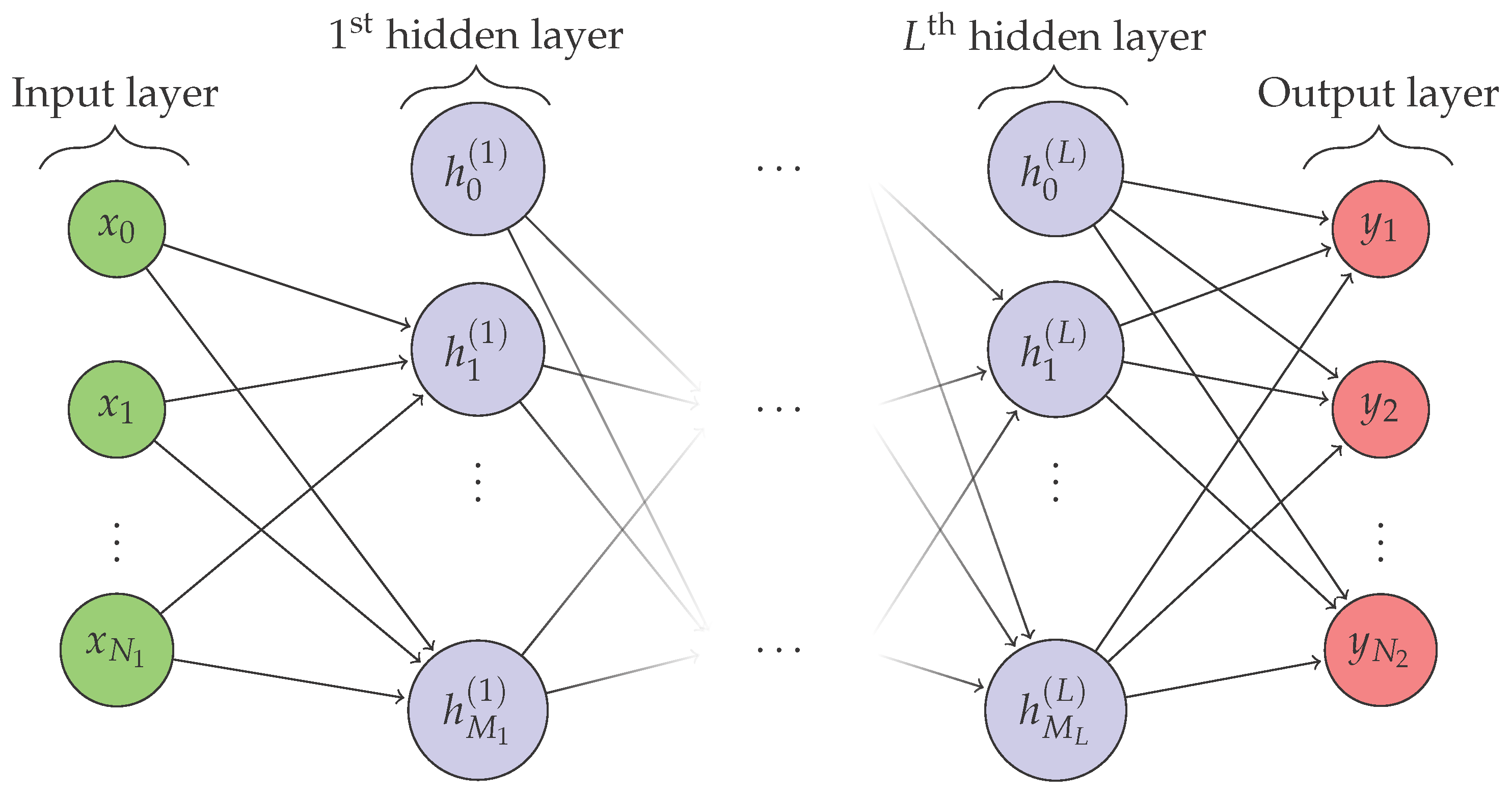
2.1.1. Introduction to ANNs

ANNs have been considered as attractive and powerful tools to predict and approximate linear, nonlinear and even complex models, based only on input-output data mapping [26,27,28]. Actually, an ANN consists of input and output layers and at least one hidden interconnection layer. A general architecture of ANN with $N_1$ inputs, $N_2$ outputs and L hidden layers is depicted in Figure 1.

ANNs can manipulate information just like the human brain thanks to the computational features of their basic units (also called nodes or neurons) which take a set of inputs, multiply them by weighted values and put them through an activation function. The schematic structure of the ith hidden artificial neuron at the jth hidden layer can be depicted as Figure 2.

There are several topologies of NNs in deep learning and they can be classified into two groups of algorithms. The first group contains the ones that were used for supervised deep learning problems such as fully-connected feed-forward algorithms (Multi-Layer Perceptron, Radial Basis Network, etc.), recurrent NNs algorithms (long short term memory, gated recurrent unit, gated feed-forward, etc.) and convolutions NNs algorithms (deep convolutional NNs, deep convolutional inverse graphics network, deconvolutional network, etc.). The second group contains the ones that were used for unsupervised deep learning problems such as restricted Boltzmann machine algorithms (deep belief network, deep Boltzmann machine, etc.) and ML auto-encoder algorithms (variational auto-encoder, denoising auto-encoder, sparse auto-encoder, etc.). However, since modelling the fuel cell is a supervised learning problem, different structures of feed-forward neural network perceptron (FFNNP) with back-propagation learning rule have been implemented in Matlab/Simulink^R and Neureal Network Toolbox^TM to predict the performance of a commercial fuel cell system (Heliocentris FC50).

2.1.2. Data Collection and Analysis

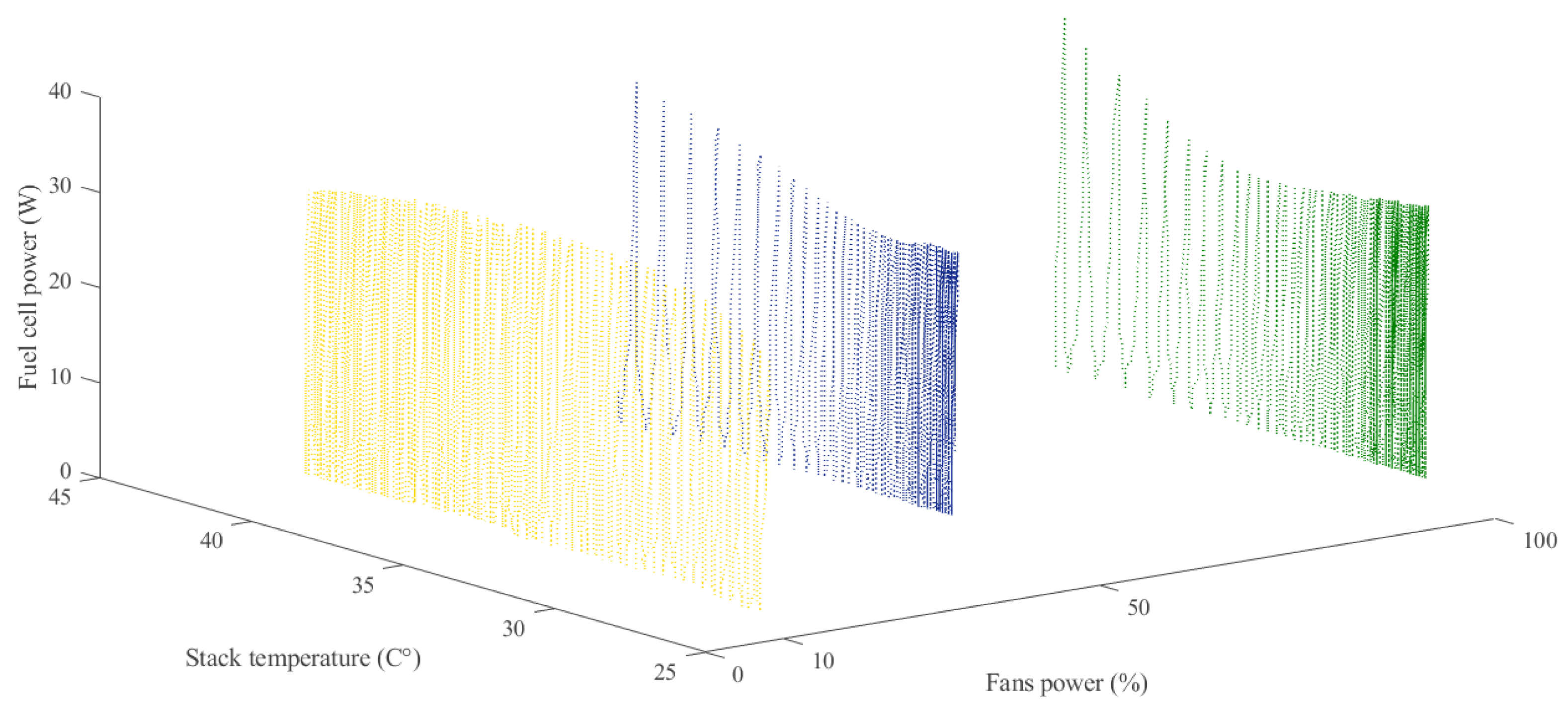
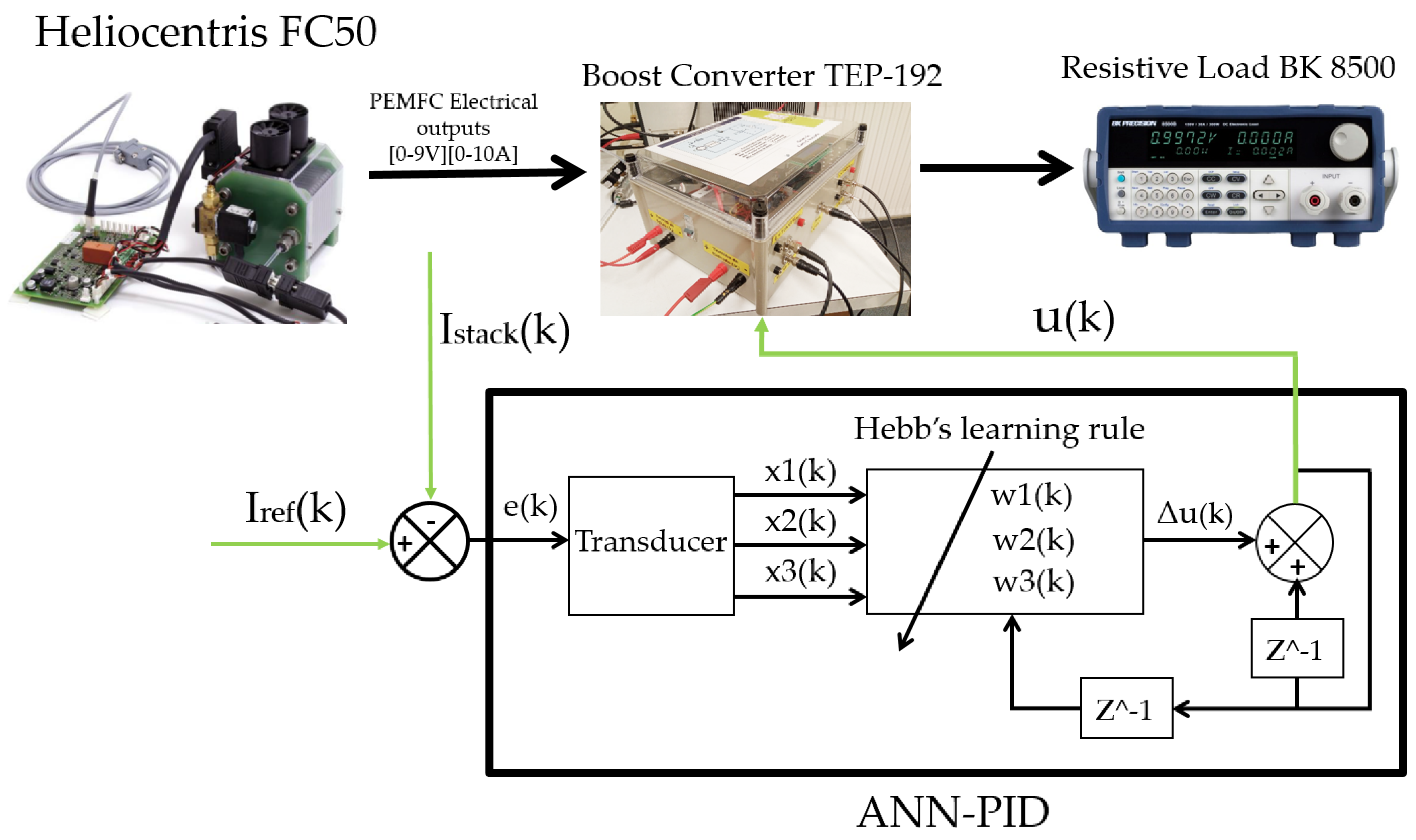
• Data collection: The first and the most important step in the supervised learning process is gathering the data. In other words, to carry out good training, vast amounts of real-world data (Big Data) is required since the more data we provide to the ML system, the faster the model can learn and improve. Besides, the collected dataset should be well distributed throughout the operation range so as to represent the behaviour of the fuel cell in each operating power point. To this end, a continuous triangular signal with a period of 15 s (7.5 s for each positive/negative slop) was built and supplied to the duty cycle of the boost converter so as to vary the stack current from the minimum to the maximum operating value. The selection of the period was made based on the characteristics of the fuel cell data acquisition software since it measures the data each 0.5 s. In other words, 15 samples in different operating current values will be measured fore each positive/negative slop. Figure 3 and Figure 4 show, respectively, the Simulink blocks used to design the triangular signal and the generated signal. The maximum value of this signal (0.8) drives the fuel cell to operate at the highest current value [8–9A] where the minimum value (0.5) drives the fuel cell to operate at the lowest operating current [0.2–0.5A]. These values can be adjusted via the increase/decrease of the output load resistance value. We have avoided operating currents above 9A since the fuel cell used in this study (Heliocentris FC50) is occupied with a security system that turns off the fuel cell in case of higher currents/temperatures [29,30,31].
  To obtain data for different operating conditions, variations in temperature, humidity, hydrogen and airflow are required. It should be noted that the fuel cell contains an integrated control system that not only controls the supplied hydrogen but also provides an option to set the fans of the fuel cell at the automatic mode. By using the auto mode, the fans will automatically control the temperature, the humidity and the supplied airflow. However, to provide large degrees of freedom, the auto mode option of the fans was not considered. Therefore, a database containing 20,512 samples for different operating current, temperature and fan power were recorded and presented in Figure 5. This latter also shows the influence of the air flow on the fuel cell performance but the effect of temperature is still not well presented. Therefore, a 3D graph that clearly shows the effect of both temperature and air flow on the stack performance is presented in Figure 6. According to this latter, it is shown that at low air flow (fans power = 10%), by varying the temperature from 25 ${}^{\circ }\mathrm{C}$ to 43 ${}^{\circ }\mathrm{C}$ the stack performance improves in the beginning, then becomes almost constant and finally, it deteriorates for higher temperatures. At medium air flow (fans power = 50%), the stack performance improves with increasing temperature. However, for higher temperatures only slight improvements occur since the membrane requires an additional amount of water content. Regarding the last case at which the air flow is set at its maximum value (fans power = 100%), the stack performance improves largely with a temperature increase from $T=$ 25 ${}^{\circ }\mathrm{C}$ to over 40 ${}^{\circ }\mathrm{C}$. It is noticed that even for higher temperatures, the stack performance is still improving and this is due to the well humidification provided by the fans.

• Inputs and outputs selection: Another factor that can improve the accuracy of the learned function is the selection of the inputs and outputs since the accuracy is strongly dependent on how the inputs are represented. The inputs should be entered as a feature vector that contains enough information to properly predict the output; but also, it should not be too large due to the dimensionality curse effect. In this study, the input variables are selected as: stack current $I_{stack}$ (A), stack temperature T (${}^{\circ }\mathrm{C}$) and fans power (%), to predict the stack voltage $V_{stack}$ (V)
• Data division (training, validation and test): When enough data is available, the next step is to split this data into three subsets which are training, validation and test. The training dataset needs to be fairly large and contains a variety of data in order to contain all the needed information. Many researchers have proposed a training set of 70%, 80% and 90% [32,33,34,35]; where the rest of data were divided between the validation and test. In this study, the recorded data was divided as the following: training = 14,358 data points (70% of whole data), validation = 3077 data points (15% of whole data) and test = 3077 data points (15% of whole data). The training subset is used to adjust the network via minimising its error. In other words, it is used for computing the gradient and updating the weights and biases of the NNs. The validation subset is used for measuring the network generalisation and to stop the training when the generalisation stops improving. In more detail, when the training begins to overfit the data, the validation error starts to rise. Therefore, the weights and biases of the network are saved at the minimum validation error point so as to balance the accuracy of the learned function versus overfitting. The test subset is used to evaluate the performance of learned function when applying a new set. Actually, the test subset has no influence on the determination of the learned function parameters, but it is a kind of ‘final exam’ to test the performance of each predicted function.

2.1.3. Designing the Network

Based on Figure 2, the output of the $h_i^{\left(j\right)}$ hidden layer unit can be calculated as Equation (1) [36].

$$h_i^{\left(j\right)}=f_{act}\left[\left(\sum _{i=0}^{M_j}{w}_{i,j}{x}_{i,j}\right)+b_i^j\right]$$

(1)

where, j = [1, 2, …, L] refers to the jth hidden layer, i = [1, 2, …, $M_j$] refers to the ith neuron in the hidden layer j, $M_j$ = [$M_1$,$M_2$, …, $M_L$] refers to the number of neurons at each layer, x∈${\mathbb{R}}^m$ are numerical inputs, w∈${\mathbb{R}}^m$ are weights associated with the inputs, b∈$\mathbb{R}$ are biases. $f_{act}$ is the activation function which is used to introduce nonlinearity into the output of the artificial neuron. Actually, this is important since most of data in the real world is nonlinear and the neurons should learn these nonlinear representations. There are many activation functions that can be used in practice such as sigmoid, tanh, ReLu, etc. [37]. In this work a tansig function which is given in Equation (2) is used.

$$f_{act}\left(x\right)=\frac{2}{1+e^{-2x}}-1$$

(2)

By using Equations (1) and (2), the kth output layer unit can be calculated as Equation (3).

$$y_k=f_{act}^{out}\left[\left(\sum _{i=0}^{M_L}{w}_{i,L}{h}_i^{\left(j\right)}\right)+b_k\right]$$

(3)

where k = [1, 2, …, $N_2$] and $f_{act}^{out}$ is a linear transfer function or also known as purelin, its mathematical expression is given in Equation (4)

$$purelin\left(x\right)=x$$

(4)

To train the FFNNP, several optimisation algorithms can be used to minimise the performance function (also known as loss/cost function) [32,38,39,40]. These algorithms use either the Jacobian of the network errors or the gradient of the network performance. Both Jacobian and gradient are computed via the back-propagation algorithm which is an efficient computational trick for calculating derivatives inside the deep feed-forward NNs. In this work, we made a comparison study among the four major used algorithms including the Levenberg–Marquardt (LM), Bayesian regularization (BR), BFGS quasi-Newton and Scaled conjugate gradient (SCG). For each training algorithm, the following basic system training parameters are used: maximum number of epochs = 5000, learning rate = 0.01, performance goal = 0, time of training = Infinity. All these parameters were checked for different number of neurons and hidden layers as presented in

Table 1. Mean squared error of different FFNNP structures/algorithms.

Training Algorithms	Hidden Layers	MSE/Time(s)	Number of Neurons for Each Hidden Layer
			1	5	10	15	20	25	30	35
LM	1	MSE	0.0241	0.0052	0.0025	0.0016	0.0017	0.0015	0.0015	0.0014
		Time	1.9520	9.3870	17.1920	6.9760	6.6720	24.9600	21.1340	16.2700
	2	MSE	0.0248	0.0036	0.0017	0.0014	0.0014	0.0012	0.0013	0.0012
		Time	8.1680	8.1740	4.4090	31.4030	29.4810	90.1620	54.3320	235.6880
	3	MSE	0.0244	0.0017	0.0015	0.0012	0.0012	0.0011	0.0011	0.0012
		Time	6.9090	10.7930	6.9720	38.5620	43.3770	304.0570	193.9730	346.6590
BR	1	MSE	0.0242	0.0106	0.0022	0.0015	0.0015	0.0015	0.0014	0.0014
		Time	4.3540	6.5850	33.0220	20.9350	40.8840	69.8870	225.6650	268.2380
	2	MSE	0.0243	0.0022	0.0014	0.0011	0.0010	0.0009	0.0008	0.0008
		Time	41.7	6.5	132.6	260.6	657.3	1583.5	2954.5	5438.6
	3	MSE	0.0243	0.0015	0.0012	0.0009	0.0008	0.0007	0.0006	0.0006
		Time	41.4	67.6	126	518.2	1064.3	4741.2	6936.3	13217.4
BFG	1	MSE	0.0245	0.0082	0.0065	0.0036	0.0030	0.0029	0.0022	0.0023
		Time	2.2560	2.4880	1.8110	4.7750	5.3230	7.8430	13.4960	7.9190
	2	MSE	0.0245	0.0088	0.0024	0.0017	0.0016	0.0020	0.0019	0.0017
		Time	1.6280	2.2800	8.2930	26.7120	25.1810	20.8690	66.0140	223.0960
	3	MSE	0.0251	0.0048	0.0053	0.0019	0.0017	0.0016	0.0018	0.0018
		Time	1.6	8.1	15.6	27.8	85.0	278.1	601.0	1125.1
SCG	1	MSE	0.0258	0.0145	0.0100	0.0090	0.0070	0.0052	0.0096	0.0070
		Time	1.2110	1.1140	1.5290	2.4660	2.8820	5.4720	2.0470	4.3250
	2	MSE	0.0261	0.0204	0.0317	0.0040	0.0041	0.0023	0.0051	0.0027
		Time	1.0180	1.0500	0.7660	5.9290	6.2720	11.5320	5.1960	27.5590
	3	MSE	0.0261	0.0082	0.0061	0.0055	0.0028	0.0025	0.0024	0.0027
		Time	1.5150	4.1530	4.7230	6.3070	12.4290	21.7610	24.7390	42.3530

.

The performance of each training algorithm was measured via the mean squared error ($mse$) which is given in Equation (5), where $y_i^{*}$ is the desired output (target), $y_i$ is the actual (predicted) output, and N is the number of dataset.

$$F=mse=\frac{1}{N}\sum _{i=0}^N{\left(e_i\right)}^2=\frac{1}{N}\sum _{i=0}^N{(y_i^{*}-y_i)}^2$$

(5)

The best performance, in terms of training time and mean squared error $mse$, of each algorithm is tinted with green colour (Table 1). The predicted output results as well as the error that corresponds to the best performance (green cells) for each training algorithm are respectively shown in Figure 7 and Figure 8.

According to these figures, it is clear that the BR training algorithm with the structure of 3 hidden layers and 30 neurons for each predicts the best output results in terms of accuracy, where the SCG shows the worst predicted results in comparison with the rest of the algorithms. In terms of time, the SCG shows the fastest training since it takes only around 11 s to predict the output while the BR needs around 6930 s. However, although the BR takes around 2 h for the training, it finally provides a highly accurate model which is one of the main goals of this study.

Figure 9 shows the regression plots which were used to validate the performance of the obtained trained model. According to this figure, it is clear that the predicted model is characterised by high accuracy since most of the data points fall along a 45 degree line, where the output is equal to the target. The goodness of the model also can be analysed via the R values which ranged between 0 (lowest accuracy) and 1 (ideal model). In our case, the accuracy of the obtained model is proven by the following R values: training, R = 0.99974, test, R = 0.99735 and all, R = 0.99938.

2.2. PEMFC Control with ANN-PID

2.2.1. Control Design

Although PID control is one of the most used controllers in industries, it still suffers from systems sufficient nonlinearity which make its constant parameters not optimal in each operating moment. This is due to the difficulties of determining the parameters which are usually tuned via the conventional trial and error method. As a solution, we have designed a self-adaptive PID based feed-forward artificial neural network (ANN-PID) aiming to avoid parameters manual tuning. The input of the ANN-PID controller is the error $e\left(k\right)$ which is achieved from the difference between the desired and actual PEMFC stack currents, and the output is the duty cycle signal $u\left(k\right)$. The error is discomposed into three variables $x_i$ (i = [1, 2, 3]) similarly to the conventional PID, but they will be respectively associated with three weights $w_i$ which are self-tuned via the Hebb supervised learning rule method. The implementation of the of ANN-PID in the hardware system is explained in Figure 10.

The output of the ANN-PID controller $\Delta u\left(k\right)$ is given in Equation (6), where k is a positive parameter determined by the user, and the values of the three inputs $x_i$ are given in Equation (7).

$$\Delta u\left(k\right)=k\sum _{i=1}^3{x}_i\left(k\right)w_i\left(k\right)=k(x_1\left(k\right)w_1\left(k\right)+x_2\left(k\right)w_2\left(k\right)+x_3\left(k\right)w_3\left(k\right))$$

(6)

$$x_i\left(k\right)=\left\{\begin{array}{c}{x}_1\left(k\right)=\Delta e\left(k\right)\hfill \\ x_2\left(k\right)=e\left(k\right)\hfill \\ x_3\left(k\right)=\Delta e\left(k\right)-\Delta e(k-1)\hfill \end{array}\right.$$

(7)

The biological origin of Hebb’s supervised learning was established from a neuroscience perspective: when two neurons are activated simultaneously, the link intensity (also called plasticity) is proportional to the multiplication of their stimulation [41,42]. Therefore, this concept can be translated mathematically for the adjustment of the PID parameters ($k_p$, $k_i$ and $k_d$) which can be obtained through a neural settlement of Equation (8) as Equation (8) shows, where ${\eta }_i$ are learning rates that correspond to $w_i\left(k\right)$ [43].

$$w_i\left(k\right)=w_i(k-1)+{\eta }_i{x}_i\left(k\right)u(k-1)e\left(k\right)$$

(8)

Recently, it has been found that the weight values used for PID online regulation are mainly related to $e\left(k\right)$ and $\Delta e\left(k\right)$[44]. Hence, the inputs $x_i\left(k\right)$ of Equation (8) can be replaced by $e\left(k\right)+\Delta e\left(k\right)$. Finally, the running algorithm of the control law can be expressed as Equation (9).

$$\left\{\begin{array}{c}{w}_i\left(k\right)=w_i(k-1)+{\eta }_i[e\left(k\right)+\Delta e\left(k\right)]u(k-1)e\left(k\right)\hfill \\ w_i^{\prime }\left(k\right)=\frac{w_i\left(k\right)}{{\sum }_{i=1}^3\left|w_i\left(k\right)\right|}\hfill \\ u\left(k\right)=u(k-1)+K\sum _{i=1}^3{w}_i^{\prime }\left(k\right)x_i\left(k\right)\hfill \end{array}\right.$$

(9)

2.2.2. Metrics Used for Control Performance Improvement

To achieve high tracking performance, the minimisation of the integral of the absolute error (IAE), the root mean squared error (RMSE) and the relative root mean squared error (RRMSE), which are described by Equation (10), have been used to adjust and tune the gains of the controller, whereas the values can be determined by taking into account the error reduction in real time.

$$\left\{\begin{array}{c}IAE={\displaystyle \sum _{i=1}^N}\left|e_i\right|\Delta t\hfill \\ RMSE=\sqrt{{\displaystyle \frac{1}{N}}{\displaystyle \sum _{i=1}^N}{\left(e_i\right)}^2}\hfill \\ RRMSE=\sqrt{{\displaystyle \sum _{i=1}^N}{\left(e_i\right)}^2/{\displaystyle \sum _{i=1}^N}\left(r_i\right)}\times 100\%\hfill \end{array}\right.$$

(10)

where N, $e_i$ and $r_i$ are, respectively, an observation data length time for the calculation, the tracking error and the reference along the i-th sample.

3. Results and Discussion

3.1. Comparison between the Experiment and Simulation Results

The $I_{stack}$-$V_{stack}$ and $I_{stack}$-$P_{stack}$ polarisation curves of the simulated and real model are presented in Figure 11. According to this figure, it is clear that the predicted model succeeded in providing the same results obtained by the real fuel cell system. It should be noted that the temperature in the experiment curves has an error around $\pm 0.5{}^{\circ }\mathrm{C}$ since it is difficult to make experiments at constant temperatures. One other variable factor that also should be taken into account is the input Hydrogen pressure which is controlled by the manufacture. However, although these two variable factors can differ the predicted results from the real ones, only slight deviations occurred.

3.2. Effect of Temperature and Humidity on the PEM Fuel Cell Stack Performance

The effects of the operation temperature on the polarisation curves for a low, medium and high humidification (fans power are set at 10%, 50% and 100%) are presented in Figure 11. At low humidification (Figure 11a,b), by varying the temperature from 25 ${}^{\circ }\mathrm{C}$ to 43 ${}^{\circ }\mathrm{C}$ the stack performance improves from $T=$ 25 ${}^{\circ }\mathrm{C}$ until $T=$ 31 ${}^{\circ }\mathrm{C}$ and then deteriorates for temperatures up to 31 ${}^{\circ }\mathrm{C}$. The improvement of the performance from $T=$ 25 ${}^{\circ }\mathrm{C}$ until $T=$ 31 ${}^{\circ }\mathrm{C}$ can be explained by the enhancement of the conductivity of the membrane which leads to reducing the activation loss. However, for temperatures above 31 ${}^{\circ }\mathrm{C}$ the membrane starts to dry due to the lack of water content which leads as a consequence to decrease the performance of the stack. At medium humidification ( Figure 11c,d), the stack performance improves with increasing temperature. However, for higher temperatures only slight improvements occurred since the membrane requires an additional amount of water content. Regarding the last case at which the membrane is 100% humidified ( Figure 11e,f), the stack performance is largely improved with increasing the temperature from $T=$ 25 ${}^{\circ }\mathrm{C}$ until $T=$ 39 ${}^{\circ }\mathrm{C}$. It is noticed that even for higher temperatures the stack performance is still improving and this is due to the well humidification provided by the fans. It should be noted that although the high humidification has a positive effect on the stack performance for higher temperatures, it also has a negative effect for lower temperatures. Hence, according to Figure 11b,f and for a low temperature equal to 25 ${}^{\circ }\mathrm{C}$, it is clear that the stack performance for low humidification ($P_{max}=33$ W) is better than the one obtained by high humidification ($P_{max}=28$ W).

3.3. Control Results

To keep the fuel cell operating at an adequate power point, PID and NN-PID are used. First, the controllers were designed and tested via the the predicted model so as to determine their coefficients. Then, they were implemented on the PEMFC hardware system using the Matlab/Simulink^TM graphical interface. To test the performance of the PID and the NN-PID, two load variations respectively from $20\Omega$ to $50\Omega$ and from $50\Omega$ to $20\Omega$ are applied during the experiments. The obtained results are clearly presented in Figure 12 and Figure 13.

The waveforms of the stack current $I_{stack}$ and voltage $V_{stack}$ are presented in Figure 12a–d and Figure 12e–h, where (b–d) and (f–h) are respectively the zoom in of a and e. The stack power $P_{stack}$ is shown in Figure 13a–d (b–d are the zoom in of a); whereas the duty cycle and the boost converter output signals (current, voltage and power) are exhibited in Figure 13e–h. According to these graphs, it is clear that both PID and NN-PID succeeded in driving the PEMFC to operate at an adequate power point even when experiencing large load variation. However, although the PID track the reference, slow motion at each load variation occurred. It takes around 6.8 s and 7.25 s to converge to the desired value (response time) respectively for the first and second load variation; whereas the NN-PID requires only 0.75 s and 0.5 s for the same load variations. Regarding the overshoots and undershoots, the PID shows an undershoot current of 2.1 A, an overshoot voltage of 1.11 V and an undershoot power of 10.21 W for the first load variation and an overshoot current of 3.65 A, an undershoot voltage of 1.33 V and an overshoot power of 8.58 W for the second load variation is displayed. On the other hand, the application of the NN-PID performs an undershoot current of 2.38 A, an overshoot voltage of 1.36 A and an undershoot power of 11.18 W for the first load variation and an overshoot current of 4.61 A, an undershoot voltage of 2.31 V and an overshoot power of 7.2 W for the second load variation. It should be noted that both experiments are made at different temperature since it is difficult to keep the fuel cell operating at a constant temperature. Since the stack current is forced via the controllers to follow the reference, the temperature effect of each experiment on the stack performance appears in the stack voltage as presented in Figure 12e–h. The steady state error of current, voltage and power for both PID and NN-PID are respectively shown in (d) and (h) of Figure 12 and (d) of Figure 13. According to these results, it is clear that the NN-PID provides better results in terms of accuracy since it reduces the amplitude of ripples from 0.1 A to less than 0.01 A. Therefore, although the PID shows slightly lower overshoots in comparison with the NN-PID, this latter provides significantly higher performance in terms of response time and steady state error.

Finally,

Table 2. Comparison of the different metrics.

IAE		RMSE		RRMSE (%)
NN-PID	PID	NN-PID	PID	NN-PID	PID
0.0049	0.0132	0.0138	0.2154	0.3440	5.3857

summarises the results of the metrics used to measure the control demeanour. It can be seen that the NN-PID achieved a better outcome in terms of the IAE since it gathered a lower value in comparison to the PID, which represents 62.8% of performance increment. In regards to the accuracy, the trend is still favourable for the NN-PID which is in contrast to the PID of 93.6%. The same situation is seen in the RRMSE since the NN-PID provided a higher improvement as 0.344% was obtained where, in comparison, the PID achieved 5.38%.

4. Conclusions

This paper presented an analysis of a commercial Heliocentris FC50 PEM fuel cell system; the objective was to model and control the device via the application of a deep machine learning based artificial neural network. Due to its several input variations, such as stack temperature, humidity and oxygen, which results in nonlinearities and high model complexity, extensive tests with various ANN parameters were required to predict an efficient model.

Since the ANN model requires a large dataset, an efficient automatic method was designed to simplify and facilitate the data collection. This was obtained by generating a triangular signal which varies the duty cycle of the power converter that was inserted between the stack and the load. An experimental dataset composed of 20,512 samples over a wide operating range (different operating current, temperature and fan power) of a commercial stack was recorded and saved for the training process.

Different structures of feed-forward neural network perceptron with backpropagation learning rule were tested to predict the performance of the Heliocentries FC50 fuel cell system. A comparison study including various ANN parameters such as the training algorithm, the number of hidden layers and the number of neurons at each layer was made to obtain the highest accurate model. Finally, an accurate model composed of 3 hidden layers and 90 neurons trained by BR algorithm was used for a comparison study with the real results. On the other hand, the predicted model also was adopted for determining the parameters of the NN-PID control method.

The effect of temperature on the PEM fuel cell stack performance was studied for low, medium and high humidification. At low humidification, it was obtained that the performance of the stack improves for low temperatures (from $T=$ 25 ${}^{\circ }\mathrm{C}$ until $T=$ 31 ${}^{\circ }\mathrm{C}$) and deteriorates for temperatures up to 31 ${}^{\circ }\mathrm{C}$. At medium and high humidifications, it was obtained that the stack performance improves with increasing temperature. However, the effect of temperature is clearly pronounced at higher humidification since the increase of temperature results in a large increase in the stack performance.

At last, two controllers were designed and performed to keep the fuel cell stack operating point at an adequate power stage. Results have demonstrated that both PID and NN-PID have succeeded in driving the stack operation to the desired power point even when experiencing large load variation. However, comparison results have shown high-performance tracking in terms of response time, and steady state error was obtained via the application of the proposed NN-PID control method.

Through this research, future trends for modelling and control of PEM fuel cell systems were analysed and will be the goal of the forthcoming studies. Other types of ANN such as recurrent neural network (RNN) can be an option to improve the performance of the model. Regarding the control method, robust and adaptive controls tuned via neural approach can be also an efficient trend to improve the tracking performance.

References

1. Li, D.; Li, S.; Ma, Z.; Xu, B.; Lu, Z.; Li, Y.; Zheng, M. Ecological Performance Optimization of a High Temperature Proton Exchange Membrane Fuel Cell. Mathematics 2021, 9, 1332. [Google Scholar] [CrossRef]
2. Mahapatra, M.K.; Singh, P. Chapter 24-Fuel Cells: Energy Conversion Technology. In Future Energy, 2nd ed.; Letcher, T.M., Ed.; Elsevier: Boston, MA, USA, 2014; pp. 511–547. [Google Scholar] [CrossRef]
3. Kadyk, T.; Winnefeld, C.; Hanke-Rauschenbach, R.; Krewer, U. Analysis and Design of Fuel Cell Systems for Aviation. Energies 2018, 11, 375. [Google Scholar] [CrossRef] [Green Version]
4. Oldenbroek, V.; Smink, G.; Salet, T.; van Wijk, A.J. Fuel Cell Electric Vehicle as a Power Plant: Techno-Economic Scenario Analysis of a Renewable Integrated Transportation and Energy System for Smart Cities in Two Climates. Appl. Sci. 2020, 10, 143. [Google Scholar] [CrossRef] [Green Version]
5. Xing, H.; Stuart, C.; Spence, S.; Chen, H. Fuel Cell Power Systems for Maritime Applications: Progress and Perspectives. Sustainability 2021, 13, 1213. [Google Scholar] [CrossRef]
6. Wang, Y.; Chen, K.S.; Mishler, J.; Cho, S.C.; Adroher, X.C. A review of polymer electrolyte membrane fuel cells: Technology, applications, and needs on fundamental research. Appl. Energy 2011, 88, 981–1007. [Google Scholar] [CrossRef] [Green Version]
7. Weber, A.Z.; Balasubramanian, S.; Das, P.K. Chapter 2-Proton Exchange Membrane Fuel Cells. In Fuel Cell Engineering; Sundmacher, K., Ed.; Academic Press: Cambridge, MA, USA, 2012; Volume 41, pp. 65–144. [Google Scholar] [CrossRef]
8. Ji, M.; Wei, Z. A Review of Water Management in Polymer Electrolyte Membrane Fuel Cells. Energies 2009, 2, 1057–1106. [Google Scholar] [CrossRef] [Green Version]
9. Han, J.; Charpentier, J.F.; Tang, T. An Energy Management System of a Fuel Cell/Battery Hybrid Boat. Energies 2014, 7, 2799–2820. [Google Scholar] [CrossRef] [Green Version]
10. Fang, L.; Di, L.; Ru, Y. A Dynamic Model of PEM Fuel Cell Stack System for Real Time Simulation. In Proceedings of the 2009 Asia-Pacific Power and Energy Engineering Conference, Wuhan, China, 27–31 March 2009; pp. 1–5. [Google Scholar] [CrossRef]
11. Saadi, A.; Becherif, M.; Aboubou, A.; Ayad, M. Comparison of proton exchange membrane fuel cell static models. Renew. Energy 2013. [Google Scholar] [CrossRef]
12. Amphlett, J.C.; Baumert, R.M.; Mann, R.F.; Peppley, B.A.; Roberge, P.R.; Harris, T.J. Performance Modeling of the Ballard Mark IV Solid Polymer Electrolyte Fuel Cell: I. Mechanistic Model Development. J. Electrochem. Soc. 1995, 142, 1–8. [Google Scholar] [CrossRef]
13. Kandidayeni, M.; Macias, A.; Boulon, L.; Trovão, J.P.F. Online Modeling of a Fuel Cell System for an Energy Management Strategy Design. Energies 2020, 13, 3713. [Google Scholar] [CrossRef]
14. Je, L.; Dicks, A. Proton exchange membrane fuel cells. Fuel Cell Syst. Explain. 2013, 18, 67–119. [Google Scholar] [CrossRef]
15. Kim, J.; Lee, S.; Srinivasan, S.; Chamberlin, C. Modeling of Proton Exchange Membrane Fuel Cell Performance with an Empirical Equation. J. Electrochem. Soc. 1995, 142, 2670–2674. [Google Scholar] [CrossRef]
16. Pathapati, P.; Xue, X.; Tang, J. A new dynamic model for predicting transient phenomena in a PEM fuel cell system. Renew. Energy 2005, 30, 1–22. [Google Scholar] [CrossRef]
17. Ansari, S.; Khalid, M.; Kamal, K.; Abdul Hussain Ratlamwala, T.; Hussain, G.; Alkahtani, M. Modeling and Simulation of a Proton Exchange Membrane Fuel Cell Alongside a Waste Heat Recovery System Based on the Organic Rankine Cycle in MATLAB/SIMULINK Environment. Sustainability 2021, 13, 1218. [Google Scholar] [CrossRef]
18. Rubio, G.A.; Agila, W.E. A Fuzzy Model to Manage Water in Polymer Electrolyte Membrane Fuel Cells. Processes 2021, 9, 904. [Google Scholar] [CrossRef]
19. Moaveni, B.; Rashidi Fathabadi, F.; Molavi, A. Fuzzy control system design for wheel slip prevention and tracking of desired speed profile in electric trains. Asian J. Control 2020, 1–13. [Google Scholar] [CrossRef]
20. Napole, C.; Barambones, O.; Calvo, I.; Derbeli, M.; Silaa, M.; Velasco, J. Advances in Tracking Control for Piezoelectric Actuators Using Fuzzy Logic and Hammerstein-Wiener Compensation. Mathematics 2020, 8, 2071. [Google Scholar] [CrossRef]
21. Tian, Y.; Zou, Q.; Han, J. Data-Driven Fault Diagnosis for Automotive PEMFC Systems Based on the Steady-State Identification. Energies 2021, 14, 1918. [Google Scholar] [CrossRef]
22. Shao, J.; Liu, X.; He, W. Kernel Based Data-Adaptive Support Vector Machines for Multi-Class Classification. Mathematics 2021, 9, 936. [Google Scholar] [CrossRef]
23. Napole, C.; Barambones, O.; Derbeli, M.; Calvo, I.; Silaa, M.; Velasco, J. High-Performance Tracking for Piezoelectric Actuators Using Super-Twisting Algorithm Based on Artificial Neural Networks. Mathematics 2021, 9, 244. [Google Scholar] [CrossRef]
24. Nanadegani, F.S.; Lay, E.N.; Iranzo, A.; Salva, J.A.; Sunden, B. On neural network modeling to maximize the power output of PEMFCs. Electrochim. Acta 2020, 348, 136345. [Google Scholar] [CrossRef]
25. Qin, Y.; Duan, H. Single-Neuron Adaptive Hysteresis Compensation of Piezoelectric Actuator Based on Hebb Learning Rules. Micromachines 2020, 11, 84. [Google Scholar] [CrossRef] [PubMed] [Green Version]
26. Vt, S.E.; Shin, Y.C. Radial basis function neural network for approximation and estimation of nonlinear stochastic dynamic systems. IEEE Trans. Neural Netw. 1994, 5, 594–603. [Google Scholar]
27. Li, Y.; Qiang, S.; Zhuang, X.; Kaynak, O. Robust and adaptive backstepping control for nonlinear systems using RBF neural networks. IEEE Trans. Neural Netw. 2004, 15, 693–701. [Google Scholar] [CrossRef] [PubMed]
28. Priddy, K.L.; Keller, P.E. Artificial Neural Networks: An Introduction; SPIE Press: Bellingham, WA, USA, 2005; Volume 68. [Google Scholar]
29. Derbeli, M.; Charaabi, A.; Barambones, O.; Napole, C. High-Performance Tracking for Proton Exchange Membrane Fuel Cell System PEMFC Using Model Predictive Control. Mathematics 2021, 9, 1158. [Google Scholar] [CrossRef]
30. Derbeli, M.; Barambones, O.; Farhat, M.; Ramos-Hernanz, J.A.; Sbita, L. Robust high order sliding mode control for performance improvement of PEM fuel cell power systems. Int. J. Hydrogen Energy 2020, 45, 29222–29234. [Google Scholar] [CrossRef]
31. Derbeli, M.; Barambones, O.; Ramos-Hernanz, J.A.; Sbita, L. Real-time implementation of a super twisting algorithm for PEM fuel cell power system. Energies 2019, 12, 1594. [Google Scholar] [CrossRef] [Green Version]
32. Karim, H.; Niakan, S.R.; Safdari, R. Comparison of neural network training algorithms for classification of heart diseases. IAES Int. J. Artif. Intell. 2018, 7, 185. [Google Scholar] [CrossRef] [Green Version]
33. Falcão, D.; Pires, J.C.M.; Pinho, C.; Pinto, A.; Martins, F.G. Artificial neural network model applied to a PEM fuel cell. In Proceedings of the IJCCI 2009: Proceedings of the International Joint Conference on Computational Intelligence, Funchal, Portugal, 5–7 October 2009. [Google Scholar]
34. Dao, D.V.; Adeli, H.; Ly, H.B.; Le, L.M.; Le, V.M.; Le, T.T.; Pham, B.T. A sensitivity and robustness analysis of GPR and ANN for high-performance concrete compressive strength prediction using a Monte Carlo simulation. Sustainability 2020, 12, 830. [Google Scholar] [CrossRef] [Green Version]
35. Nhu, V.H.; Hoang, N.D.; Duong, V.B.; Vu, H.D.; Bui, D.T. A hybrid computational intelligence approach for predicting soil shear strength for urban housing construction: A case study at Vinhomes Imperia project, Hai Phong city (Vietnam). Eng. Comput. 2020, 36, 603–616. [Google Scholar] [CrossRef]
36. Arabi, M.; Dehshiri, A.; Shokrgozar, M. Modeling transportation supply and demand forecasting using artificial intelligence parameters (Bayesian model). Istraz. I Proj. Za Privredu 2018, 16, 43–49. [Google Scholar] [CrossRef] [Green Version]
37. Mudunuru, V. Comparison of activation functions in multilayer neural networks for stage classification in breast cancer. Neural Parallel Sci. Comput. Arch. 2016, 24, 83–96. [Google Scholar]
38. Kumar, D.A.; Murugan, S. Performance Analysis of MLPFF Neural Network Back Propagation Training Algorithms for Time Series Data. In Proceedings of the 2014 World Congress on Computing and Communication Technologies, Trichirappalli, India, 27 February–1 March 2014; pp. 114–119. [Google Scholar] [CrossRef]
39. Sharma, B.; Venugopalan, K. Comparison of Neural Network Training Functions for Hematoma Classification in Brain CT Images. IOSR J. Comput. Eng. 2014, 16, 31–35. [Google Scholar] [CrossRef]
40. Shende, K.V.; Kumar, M.R.; Kale, K. Comparison of Neural Network Training Functions for Prediction of Outgoing Longwave Radiation over the Bay of Bengal. In Computing in Engineering and Technology; Springer: Berlin/Heidelberg, Germany, 2020; pp. 411–419. [Google Scholar]
41. Meng, F.; Hu, Y.; Ma, P.; Zhang, X.; Li, Z. Practical Control of a Cold Milling Machine using an Adaptive PID Controller. Appl. Sci. 2020, 10, 2516. [Google Scholar] [CrossRef] [Green Version]
42. Magotra, A.; Kim, J. Improvement of Heterogeneous Transfer Learning Efficiency by Using Hebbian Learning Principle. Appl. Sci. 2020, 10, 5631. [Google Scholar] [CrossRef]
43. Napole, C.; Barambones, O.; Calvo, I.; Velasco, J. Feedforward Compensation Analysis of Piezoelectric Actuators Using Artificial Neural Networks with Conventional PID Controller and Single-Neuron PID Based on Hebb Learning Rules. Energies 2020, 13, 3929. [Google Scholar] [CrossRef]
44. Liang, Y.; Xu, S.; Hong, K.; Wang, G.; Zeng, T. Neural network modeling and single-neuron proportional–integral–derivative control for hysteresis in piezoelectric actuators. Meas. Control 2019, 52, 1362–1370. [Google Scholar] [CrossRef]
Figure 1. Network graph of N 1 input units, N 2 output units and L-layer perceptron where each hidden layer contains M j hidden units.Network graph for a L-layer perceptron.
Mathematics 09 02068 g001
Figure 2. Structure of a single artificial neuron in a neural network.
Mathematics 09 02068 g002
Figure 3. Triangular signal design.
Mathematics 09 02068 g003
Figure 4. Triangular signal output.
Mathematics 09 02068 g004
Figure 5. I s t a c k - P s t a c k and I s t a c k - V s t a c k measured data of Heliocentris FC50 fuel cell; (a,d): polarisation curves when Fans Power = [10%, 20%, 30%] and for different operating temperature; (b,e): polarisation curves when Fans Power = 50% and for different operating temperature; (c,f): polarisation curves when Fans Power = 100% and for different operating temperature.
Mathematics 09 02068 g005
Figure 6. The Heliocentris FC50 stack power according to air flow and stack temperature.
Mathematics 09 02068 g006
Figure 7. Predicted output results when using SCG, BFG, LM and BR.
Mathematics 09 02068 g007
Figure 8. Obtained training errors when using SCG, BFG, LM and BR.
Mathematics 09 02068 g008
Figure 9. Performance analysis of the predicted model.
Mathematics 09 02068 g009
Figure 10. Implementation of ANN-PID on Heliocentris FC50 hardware system.
Mathematics 09 02068 g010
Figure 11. Simulation and experiment results (simulation: continuous line; experiment: dashed line); (a): I s t a c k - V s t a c k polarisation curves when Fans Power = 10%; (b): I s t a c k - P s t a c k polarisation curves when Fans Power = 10%; (c): I s t a c k - V s t a c k polarisation curves when Fans Power = 50%; (d): I s t a c k - P s t a c k polarisation curves when Fans Power = 50%; (e): I s t a c k - V s t a c k polarisation curves when Fans Power = 100%; (f): I s t a c k - P s t a c k polarisation curves when Fans Power = 100%.
Mathematics 09 02068 g011
Figure 12. PID and NN-PID experimental results; (ad): PEMFC stack current signal; (eh): PEMFC stack voltage signal.
Mathematics 09 02068 g012
Figure 13. PID and NN-PID experimental results; (ad): PEMFC stack power signal; (e): Duty cycle signal (f): Boost converter output current; (g): Boost converter output voltage; (h): Boost converter output power.
Mathematics 09 02068 g013