Abstract
In a series of three articles, spline approximation is presented from a geodetic point of view. In part 1, an introduction to spline approximation of 2D curves was given and the basic methodology of spline approximation was demonstrated using splines constructed from ordinary polynomials. In this article (part 2), the notion of B-spline is explained by means of the transition from a representation of a polynomial in the monomial basis (ordinary polynomial) to the Lagrangian form, and from it to the Bernstein form, which finally yields the B-spline representation. Moreover, the direct relation between the B-spline parameters and the parameters of a polynomial in the monomial basis is derived. The numerical stability of the spline approximation approaches discussed in part 1 and in this paper, as well as the potential of splines in deformation detection, will be investigated on numerical examples in the forthcoming part 3.
Keywords:
spline; B-spline; polynomial; monomial; basis change; Lagrange; Bernstein; interpolation; approximation; least squares adjustment 1. Introduction
In engineering geodesy, the use of point clouds derived from areal measurement methods, such as terrestrial laser scanning or photogrammetry, results in the necessity to approximate them by a curve or surface that can be described using a continuous mathematical function, often by means of splines. In part 1 of a three-part series of articles, presented by Ezhov et al. [1], the basic methodology of spline approximation was shown by means of ordinary cubic polynomials concatenated under constraints for continuity, smoothness, and continuous curvature. The resulting linear adjustment problem can be solved within the Gauss-Markov model with constraints for the unknowns.
However, a starting point for advanced considerations in engineering geodesy are almost always the formulas for B-spline curves and B-spline surfaces given in the textbook by Piegl and Tiller [2] (pp. 81 and 100), where the functional values of the B-spline basis functions are recursively computed according to the formulas by de Boor [3] and Cox [4]. As these formulas have a very complex mathematical derivation, but are still very easy to use, they are mostly used like a given recipe. Attempts to explain B-splines in an illustrative way often only include explanations of the application of the de Boor’s algorithm, as, for example, in the contribution by Lowther and Shene [5]. A derivation of the B-spline with the help of quadratic Bézier spline curves was presented by Berkhahn [6] (p. 73 ff.).
In this paper, we take the spline representation presented by Ezhov et al. [1] as a starting point to derive the B-spline form by means of basis changes. This is to show the user that the de Boor’s algorithm can be interpreted as another, very elegant and numerically stable, representation of the simple and intuitive representation based on ordinary polynomials.
A brief overview of the historical development of the B-spline can be found, for example, in the textbook by Farin [7] (p. 119). He explains that the forerunner of the B-spline first appeared in a publication on approximation theory by the mathematician Lobatschewsky [8]. It was constructed as a convolution of certain probability distributions. However, at that time the term “spline” has not been introduced yet. Subsequently, in 1946, Schoenberg used B-splines in his seminal publications [9,10] for data approximation. It is commonly accepted that, with these articles, the modern representation of spline approximation began and the term “spline” was used for the first time, see the historical notes in the textbook by Schumaker [11] (p. 10). Further on, many authors dealt with the utilization and the development of the B-splines. Farin [7] (p. 119) points out that one of the most important developments in this theory was the introduction of the recurrence relations, discovered by de Boor [3], Cox [4], and Mansfield. The contribution of Mansfield to this development is mentioned by de Boor in [3]. However, the recurrence relation had already appeared in contributions by Popoviciu and Chakalov in the 1930s, see the article by de Boor and Pinkus [12] and the literature cited therein.
B-splines were later fully exploited in computer graphics. Consequently, most papers about B-splines were published in this field, see for example, the contributions by the authors Piegl and Tiller [2], Szilvasi-Nagy [13], Farin [7], and Zheng et al. [14]. However, there are several publications where B-splines were used for statistical data analysis, e.g., the contributions by Wold [15] or Anderson and Turner [16].
Applications of (B)-splines in geodesy can be traced back to 1975, when Sünkel began using them for various problems. In [17], bicubic spline functions were used for the reconstruction of functions from discrete data. In [18], the representation of geodetic integral formulas by bicubic spline functions was shown using splines constructed from ordinary cubic polynomials, see [18] (p. 10 ff.), similar to the representation used later by Ezhov et al. [1]. In [19], the local interpolation of gravity data by spline functions was derived, and in [20] (p. 18 ff.) B-splines were used for smooth surface representation. As references for the B-spline functions, the publications of Schoenberg [21], Schumaker [22], and Späth [23] are listed by Sünkel [20].
On the basis of B-splines on the line, Jekeli [24] (p. 7 ff.) showed the use of spherical B-splines for representations of functions on a sphere for geopotential modeling. Mautz et al. [25] used B-splines to develop a representation of global ionosphere maps based on B-spline wavelets. The local improvement of the International Reference Ionosphere (IRI) by means of an N-dimensional B-spline surface was developed by Koch and Schmidt [26].
The application of (B)-splines in engineering geodesy can be traced back to 1985, when Dzapo et al. [27] used cubic splines for the determination of the lengths of railroad tracks. A recent application of B-spline curves and B-spline surfaces is the approximation of 3D point cloud data, as shown e.g., by Bureick et al. [28]. Kermarrec et al. [29] applied hierarchical B-splines for the approximation of 3D point cloud data obtained from measurements with a terrestrial laser scanner. Furthermore, B-spline models play an important role in spatio-temporal deformation analysis as shown by Harmening [30].
The main goal of this paper is to present an alternative derivation of the B-spline function to the purely mathematical derivation presented by Schoenberg [9] and the recursion formulas for the B-spline function developed by de Boor [3]. This derivation is based on the transition from the representation of a polynomial in the monomial basis (ordinary polynomial) to the Lagrangian form and, from there, to the Bernstein form, which finally results in the B-spline representation. In all investigations, univariate splines are used in form of a spline function . For the derivation of the formulas, we first consider the case of interpolation. The developed formulas are then used for spline approximation using least squares adjustment.
The general interpolation problem is, to find for given data points , , …, , with a function in such a way that the interpolation condition
is fulfilled. The choice of a suitable function depends on the properties of the data, e.g., its smoothness or periodicity. Furthermore, the choice of is influenced by computational aspects, i.e., the computational effort for the determination of the coefficients and numerical stability of the resulting equation system. Functions that are commonly used for interpolation are:
- -
- Polynomials;
- -
- Trigonometric functions;
- -
- Exponential functions;
- -
- Logarithmic functions;
- -
- Rational functions.
Ezhov et al. [1] elaborated a spline approximation using piecewise ordinary cubic polynomials. In the following, we will take a closer look at the interpolation using polynomials in different representations to bridge the gap to the B-spline representation.
In general, the set of functions for interpolating given data points consists of coefficients and so-called basis functions and the interpolating function is defined as a linear combination
of these basis functions. Considering the interpolation condition (1), we obtain
The simplest and most common type of interpolation uses polynomials. These polynomials can be represented in different ways, as shown by Gander [31], but all of them will give the same result for the interpolation.
To avoid excessive formula derivations and to illustrate the geometric relationships in the formula derivations, quadratic splines that consist of piecewise parabola segments are considered in the following. The generalization to splines of a higher degree is relatively straightforward.
Using the example of a parabola, we start with the representation of a polynomial in the monomial basis (ordinary polynomial) and perform the following transitions:
The reason for the representation of a polynomial in a different basis than the well-known monomial basis applied by Ezhov et al. [1] often lies in the fact that for the computation of the polynomial coefficients equation systems result, whose solution requires less computational effort and is numerically more stable. However, it is important to understand that the change of the basis functions still results in the same interpolating polynomial for the given data, and only the representation of the polynomial changes. After the derivation of the B-spline representation, this form is used for spline approximation using least squares adjustment (Section 5). The interesting fact that the determined spline parameters can be used for a transition “backwards” from B-spline to ordinary polynomial is shown in Appendix A. The transition “forwards” from ordinary polynomial to B-spline is shown in Appendix B.
2. Transition from Ordinary Polynomial to Lagrangian Form
A polynomial in the monomial basis is often referred to as standard form or ordinary polynomial. Arranging the monomials in a vector and the coefficients in a vector , we obtain
A visualization of the monomial functions for the parabola is shown in Figure 1.
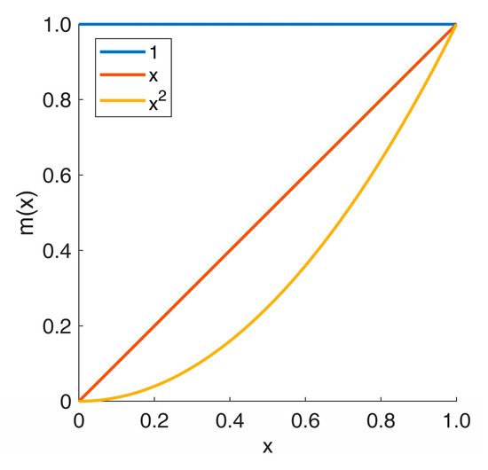
Figure 1.
Monomial basis functions for a parabola in the interval [0, 1].
Considering the interpolation condition (1), the coefficients can be determined from the solution of the linear equation system
with and the Vandermonde matrix
cf. the textbook by Farin [7] (p. 100). Using a numerical example with three points that define a parabola from the handbook by Bronshtein et al. [32] (p. 918), see Table 1, the determination of the coefficients will be demonstrated.

Table 1.
Numerical example for interpolating a parabola.
From Equation (7), we obtain for this numerical example
This system of equations can be solved with, for example, the Gaussian elimination method and the numerical result is , , . Thus, the equation of the parabola reads
It can be stated that, when using the monomial basis, the numerical effort to determine the coefficients requires roughly operations using direct methods for solving systems of linear equations, as stated e.g., by Farin [7] (p. 102), and is therefore comparably high. It can be reduced by employing iterative methods. In addition, the matrix of the equation system is increasingly ill-conditioned as the degree of the polynomial increases. Both the conditioning of the resulting linear equation system and the computational effort for determining the coefficients can be improved by using other basis functions. The result is the same interpolating polynomial, but in a different representation.
In the following subsections we will illustrate two ways how to perform a transition from the monomial basis to a representation with Lagrange polynomials.
2.1. Transition by Means of Basis Transformation
We want to solve the problem of basis transformation between two different sets of coefficients and fulfilling
where and are two different sets of basis functions. Using the monomial basis function (4) in the first summation formula, we obtain
as already shown in (5) and (6). Multiplying out the second summation formula in (11) yields
and, according to (11), we can write
In the case of monomial basis, we selected basis functions and obtained the coefficients, see (7), while here we do the opposite. We select , , for the coefficients to obtain corresponding basis functions for which we introduce the new notation with . Furthermore, for we introduce the solution according to (7) and we obtain
By comparing the coefficients of the vectors , we see that the basis functions can be computed from
Introducing the vector yields
The same formula can also be obtained taking the basis transformation from Lagrange to monomials , as presented by Gander [31], and solving it for . From (17), we obtain the result
which is called the Lagrange basis. A visualization of the Lagrange basis functions for the parabola is shown in Figure 2.
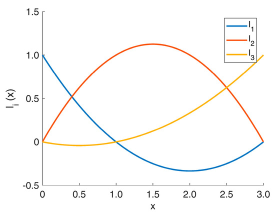
Figure 2.
Lagrange basis functions for a parabola in the interval [0, 3] for the example , and .
Finally, the resulting polynomial reads
An alternative derivation of the Lagrange representation of a polynomial is presented in the following subsection.
2.2. Transition by Linear Combinations
In this subsection, we present an alternative derivation of the polynomial in the Lagrange representation. We use the fact that each parabola can be represented as a combination of two lines. In fact, if we take a look at (5), we find that it can be rearranged into the form , which represents a combination (product) of two lines plus some constant value . By using this idea, the Lagrange representation of a quadratic polynomial can be derived, which results in a linear combination of three quadratic functions and the respective coordinates.
We consider the points , where . Now two lines
within the interval and
within the interval are defined, see Figure 3. The subscripts and in represent the number of the polynomial for a given degree .
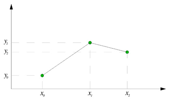
Figure 3.
Line interpolation.
From two given points, the slope of the line (20) can be written as
The y-intercept can be computed from
Analogously, the equation for the second line can be written as
By taking a combination of these two line equations, where varies within the interval , the expression
for the parabola is derived, which represents a linear combination of three quadratic polynomial functions and the coordinates , and .
To explain how the factors in front of the terms and in (26) are derived, the idea behind the Lagrange polynomials has to be explained. Lagrange was looking for an interpolation polynomial that could be constructed without solving a system of equations, e.g., with Vandermonde matrix as design matrix, see (7). There is a widely accepted assumption that his idea for the solution was to find a function that, at each given data point , , …, , gives 1 and, at the rest of the other given points gives 0. For a mathematician, this type of polynomials was, presumably, relatively easy to find. We will take the case of a parabola into consideration. Therefore, for each given , the following polynomials
can be created.
As previously mentioned, these functions are equal to 1 when the variable is equal to the corresponding coordinate of the given point and 0 at all other given points. Therefore, by multiplying each of these functions with their corresponding values ensures that, at the particular given point , the result will be and 0 at all other given points. The summation of all these functions , multiplied by their corresponding values , results in a Lagrangian interpolation polynomial
The quadratic polynomial (30) represents a linear combination of the Lagrangian basis polynomials with the constants , and as coefficients. A general formula for the definition of the Lagrange interpolation polynomials can be found e.g., in the handbook by Bronshtein et al. [32] (p. 918).
As previously explained, a quadratic polynomial can be represented as a combination of two lines. Using the Lagrangian form for a polynomial of first order, the following two line equations
are derived. If we follow the already described Lagrange’s idea to obtain a quadratic polynomial, the following multiplications
must be performed.
Consequently, Equation (33) results in a Lagrangian polynomial of second order. Looking at (33), the factors and are those that appear in front of the terms and in (26). However, if we compare the Lagrange polynomials in (31), (32), (33) with the expressions in (24), (25), (26), the only difference is that (31), (32) and (33) have negative denominators and numerators at some points in the Lagrange polynomials, e.g. . In (24), (25) and (26) there are no negative denominators or numerators, although the equations are the same as in (31), (32) and (33). This is for reasons of better analogy with the B-spline form.
After the origin of the factors in front of and in (26) is explained, inserting (24) and (25) into (26) finally yields
This form coincides with (19) and represents a second degree Lagrange interpolating polynomial through three points, see the handbook by Bronshtein et al. [32] (p. 918). The plot of the parabola is depicted in Figure 4.
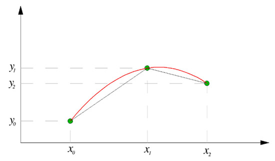
Figure 4.
Lagrange interpolation by lines (black) and by a parabola (red).
Inserting the values of the numerical example from Table 1 into (34) yields the Lagrangian form
which can be “simplified” to the monomial basis form
The result is the same as in (10), but the values of the parameters , , are now derived with the advantage of not explicitly solving a linear equation system. A disadvantage of Lagrange interpolation in practical application is directly visible from (19), resp. (34), namely that each time a value changes, the Lagrange basis polynomials must be recalculated. Further general limits of Lagrange interpolation, e.g., that polynomial interpolants may oscillate, are explained by Farin [7] (p. 101 ff.).
3. Transition from Lagrangian Form to Bernstein Form
The Bernstein form, named after S. N. Bernstein, was used to prove the Weierstrass approximation theorem; see the explanation by Farin [7] (p. 90 ff.). The coefficients of a Bernstein polynomial over the interval [0, 1] are all non-negative and sum up to 1, as Farin [7] (p. 57 ff.) showed, which is called a convex combination; see the textbook by Rockafellar [33] (p. 11). Therefore, by using the Bernstein form, numerical instabilities are avoided.
Looking at Figure 3, the interpolating parts of the line segments can be extended to both ends of the interval in which the polynomial is defined. At the end of the extended line segments, two additional y-coordinates for the values and are computed, as seen in Figure 5. To distinguish these two y-coordinates from the given values, a different notation, and , is used (not to be confused with the derivation of a function). In a general case, all five points have different coordinates which implies that the coordinate is not necessarily in the middle of the interval . Therefore, in general .
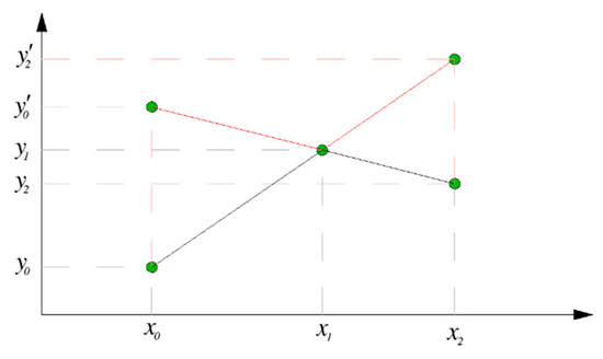
Figure 5.
Extended line segments from Lagrangian form.
From Figure 5, as explained previously, the line equations
are derived. By taking combinations of these two lines, it follows
which can be brought into the form
A geometrical interpretation of the term is depicted in Figure 6.
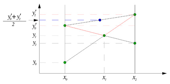
Figure 6.
Geometrical interpretation of the term .
Equation (39) is a more general representation of the Bernstein form, independent of the limits of the interval , which means that can vary between any two real values. For proving the Weierstrass approximation theorem, Bernstein used a special interval of length 1, i.e., . Using this interval simplifies the equations, which were later used by Bézier and de Casteljau. Therefore, when using , Equation (37) results in
and (39) obtains the form
in which , and are the Bernstein basis polynomials and , and are the Bernstein coefficients. In general, a polynomial in Bernstein form of degree can be written as
where are the Bernstein coefficients and
are the Bernstein basis polynomials; see e.g., the handbook by Bronshtein et al. [32] (p. 935). For a parabola, we obtain , and , cf. (41). These basis polynomials for a parabola are depicted in Figure 7.
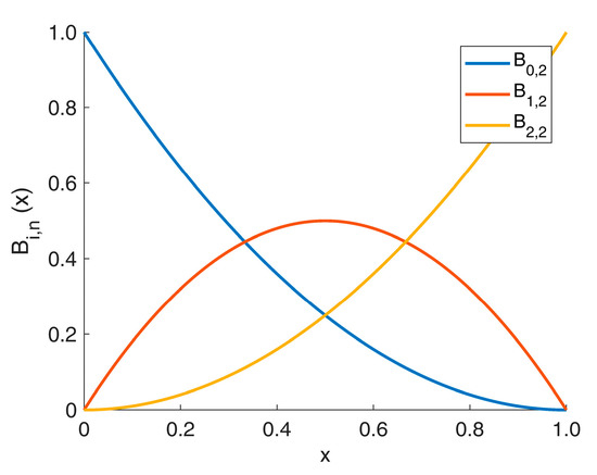
Figure 7.
Bernstein basis polynomials for a parabola in the interval [0, 1].
In (39), the term , see Figure 6, reveals one fundamental property of the quadratic polynomial that, to the best of our knowledge, is not described in the literature so far. It can be stated as:
All pairs of line segments that have one end fixed at the beginning or at the end of the parabola and the other end at the opposite sides of the interval, and intersect themselves on the parabola, have an equal average of the coordinates at the ends that are not fixed. Moreover, the extremum of the parabola lies on the intersection of those line segments that have equal values at the opposite ends of the interval.
The proof of this statement is straightforward. A parabola is uniquely defined by three points. If we retain end points and , replacing the point by any other point on the same parabola, we will again obtain the equation of the form (39). The equation of the parabola remains unchanged although and have changed, since the only term depending on the new point is . A parabola is described by a differentiable function. By computing its derivative, equating it with zero and solving the resulting equation for , we obtain the coordinate of the extremum . Consequently, the resulting equation for the coordinate of the extremum can be solved. By substituting these two values for and in a line equation constructed for and , where and respectively, it can be shown that . Therefore, implies . This proves the above statement, which is illustrated in Figure 8. and represent the fixed points at the beginning and at the end of the parabola, with and as end points at the opposite sides of the interval. Every pair of line segments is defined as , , , …, and depicted in light blue color. Figure 8 illustrates that all these pairs of line segments intersect on the parabola.
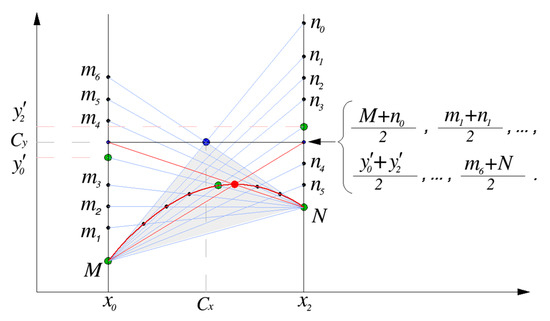
Figure 8.
Construction of a Bernstein polynomial. The extremum of the parabola is marked with a red dot and the control point with a blue dot. Green dots indicate points on the parabola, resp. points resulting from extension of straight lines between these points to the boundaries of the interval . The convex hull formed by the control points , and is highlighted in grey.
Considering the above, there are an infinite number of combinations defining the term depending on the position of the point , between and , that defines the parabola, cf. Figure 6. All of these pairs of line segments, as previously explained, have an equal average of the y-coordinates at the end points. Therefore, the term that uniquely represents all these averages is written more generally in the form
where and represent any pair of -coordinates from the mentioned line segments that intersect on the parabola. Correspondingly, the coordinate is defined as
where and define the ends of the interval in which the parabola varies. Hence, is always in the middle of the interval.
There is an additional property of the line segments and . They intersect at the point and are tangential to the curve. This can be easily proven. We can compute the first derivative and solve for and from (44), then construct two line equations for and and solve for their intersection.
In the context of geometric modelling, the point defined by is called control point and, concerning basis splines (B-splines), it is named de-Boor-point. In Figure 8, this point is marked with a blue dot. Moreover, the first and the last point of the parabola are also referred to as control points, see e.g., the textbook by Piegl and Tiller [2] (pp. 389–390).
As a more general representation of the Bernstein polynomial, (46) is a convex combination as well. The proof is obvious. Since , all functions in front of , and are non-negative and have a sum of 1. The control points , and form a convex hull, highlighted in grey in Figure 8, that encloses all realizations of in (46), which means that all points of the parabola lie within the convex hull. A convex hull is the smallest convex set that contains a given set, with a convex set being a set wherein the straight line segment, connecting any two points of the set is completely contained within the set; see e.g., the textbook by Farin [7] (p. 439). The advantage of the general representation of the Bernstein polynomial is that it can be applied directly without scaling the data set to the interval .
If we now consider the example from Table 1 once again, we get, with and , from (44) the result and therefore
which can be “simplified” to the monomial basis form
For the case of the interpolation by a parabola, it can be concluded that both the Bernstein and the Lagrangian form yield the same result. However, the Bernstein form has the advantage that all points of the parabola lie in the convex hull defined by its parameters.
4. Transition from Bernstein Form to B-spline
In the previous section, the Bernstein form was derived with a more general approach, instead of the standard representation within the interval . This form can be easily used for derivation of the B-spline.
In this section, Equation (46) is used for further derivations. It is assumed that the line segments that define the quadratic polynomial intersect at the extremum of the parabola and have an identical coordinate . Since the notion of spline is to be explained, only the endpoints of two smoothly connected parabolas are considered, which are better known as knots , and . The problem of the constraints and how they are imposed on the spline, for spline interpolation, is not taken into consideration. It is presumed that the first parabola of the spline is already defined, e.g., by imposing a constraint for the direction of the tangent in point as boundary condition, and in this case, is identical with the one from the previous section, see Figure 8.
The initial situation is depicted in Figure 9, where:
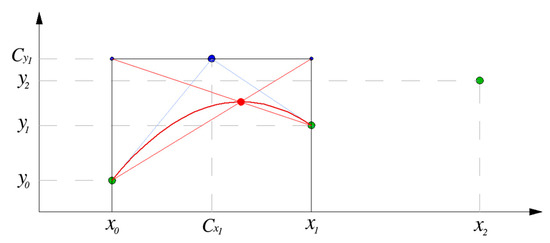
Figure 9.
Initial situation before the construction of the second part of the spline. The extremum of the first parabola is marked with a red dot, the control point with a blue dot, and the green dots indicate points to be interpolated.
- -
- One parabola already exists between the knots and ; and
- -
- One knot is given that is to be interpolated.
The task is now to construct a second parabola between the knots and which is tangential to the first one.
The second parabola is constructed as follows:
- -
- The line segment is extended from the end point of the parabola to the end of the interval , yielding the additional coordinates and therefore the new line segment , see Figure 10;
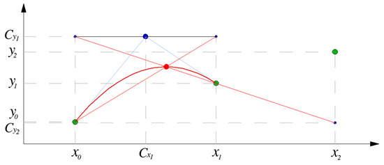 Figure 10. Line segment . The extremum of the first parabola is marked with a red dot, the control point with a blue dot, and the green dots indicate points to be interpolated.
 - -
- Between points and , the line segment can be constructed, see Figure 11;
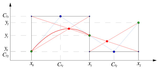 Figure 11. Line segment . The extrema of the parabolas are marked with a red dot, the control points with a blue dot, and the green dots indicate points to be interpolated.
 - -
- By taking combinations of these two line segments, within the interval , another parabola will be constructed, smoothly connected to the previous one. The whole function constructed from these two smoothly connected parabolas represents a spline. Both parabolas end tangentially at the point w.r.t the line segment, defined as , see Figure 12.
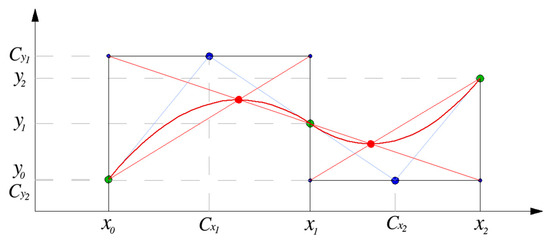 Figure 12. Second parabola within the interval , smoothly connected to the previous one. The extrema of the parabolas are marked with a red dot, the control points with a blue dot, and the green dots indicate points to be interpolated.
Finally, this is a type of spline that is constructed by using convex combinations and it is exactly the same as the B-spline. This is shown by the equations derived further in the text. Algebraically, this derivation is similar to the one in the previous section. The first pair of line equations is written as
By taking a combination of these two lines within the interval , it follows
For the second parabola the same approach is applied. The second pair of line equations is defined in the same way as the previous one, yielding
Analogously to (50), but in this case within the interval , we obtain
If the above derived expressions are compared to an explicit expression of a quadratic B-spline it becomes clear that they are the same. However, for the sake of clarity we have used a particular notation that does not correspond to the usual B-spline notation.
Looking at (50) and (52), the only unknowns are and , all other values are given. It appears that a quadratic spline, constructed from two linear polynomials, can be estimated with only two equations. This type of reasoning would lead to a paradox. Therefore, for this type of a spline, since all constraints (smoothness and continuity) are hidden inside the equations, at least four observations are necessary for a solution. For comparison, a spline constructed from two polynomials of the form requires at least three observations and three constraints.
The idea presented in this section can be used for constructing splines of higher degrees as well. In those cases, depending on the degree of the spline, one would need more knots and more control points for creating a spline segment, while the number of combinations increases. Moreover, the expressions became more complicated, which makes this approach unsuitable for practical applications. However, de Boor [3] developed an algorithm for computing the basis functions that, in our case, constructs the expressions in front of the coordinates of the control points in (50) and (52).
De Boor’s algorithm is based on the Cox-de Boor recursion formula that we will use for explaining the computation of a B-Spline. Recursion itself is non-intuitive, which makes this formula difficult to be explained analytically. The higher the degree of the spline, the more cumbersome and harder to follow the equations become. Therefore, in order to make a comparison with (50) and (52), we will use an explicit expression of a quadratic B-spline that is derived from the Cox-de Boor recursion formula. For this purpose, we use the knots and the naming convention from the previous example (49)–(52). For this formula to work, we have to rename the parameters (control points) to and to . The Cox-de Boor recursion requires additional knots at the beginning and at the end of the spline based on the degree of the spline. If the spline degree is , two additional knots are presumed to be both at the beginning and at the end of the spline. In our case, they are
which is called knot multiplication. Additional knots with e.g.,
are especially used to gain endpoint interpolation. The additional knots do not necessarily have to be equal to and , they are just required to follow the order and . However, in our example we follow the convention of the knot multiplication, and because of the knot multiplication, formula (56) has zero divisions, and the solution for this problem is to declare that “anything divided by zero is equal to zero”.
The base case of the recursion formula is
with a recursive step to compute the basis functions
which is summed over the k-th interval of the spline , such as
At the beginning of the recursion (56), index denotes the degree of the spline and is a computed index . In each recursive step, is lowered down for 1 until it reaches 0. At , the recursion formula terminates and the base case (55) is evaluated.
The index is the index of the interval with , where is the number of knots. Therefore, for , the recursion formula (56) is computed for every of the sum (57) and evaluated in (55). Afterwards, for , the same computation is performed, and so on, until the last interval. The parameters in (57) correspond to each basis function terminated by in (55) at the end of the recursion. An example of quadratic basis functions using the knots , and , resulting in two intervals and , and the knot sequence , is shown in Figure 13.
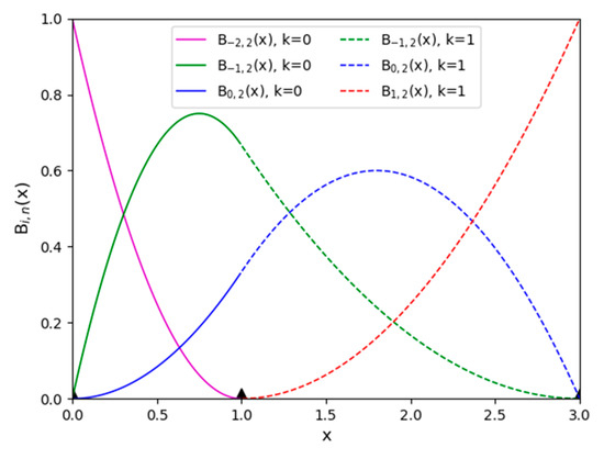
Figure 13.
Quadratic B-Spline basis functions using the knots , and , resulting in two intervals and , and the knot sequence . The knots are marked with black triangles on the x-axis.
To compare this approach with (50) and (52), we use an explicit expression of a generic quadratic B-spline formula. For deriving it, we consider in (56), then we follow all recursive steps until for every , which yields the explicit expression of a generic quadratic B-spline formula
For clearer description, we treat each part of (57) separately and, for the computation, we use the knot sequence (53). At the interval , with index , the first element of the sum is
With , the second element of the sum is
and, with , the last element of the sum is
Taking the knot multiplications (53) and (54) into account for all elements of the sums (59)–(61) yields
The base case (55) evaluates only the functions in front of , all other base functions are not taken into consideration nor are the fractions where division by zero occurred. Finally, by summing up all results (62), (63) and (64) for the first interval, as stated in (57), and evaluating by (55), we obtain
If Equation (65) is compared to (50), it can be concluded that they are identical. It must just be taken into consideration, as stated previously, that is renamed to . If the same procedure is applied to , the result is identical to (52), considering that is renamed to .
Since spline functions are considered, only the component of a control point appears as a factor in front of the basis functions . Using a parametric spline curve, both components of a control point appear in front of the basis functions as e.g., applied by Bureick et al. [34].
5. B-spline Approximation
As pointed out by Ezhov et al. [1], in engineering geodesy it is not appropriate to apply a spline interpolation due to the high point density and the fact that measurements are affected by random measurement errors. Observation errors and other abrupt changes in the data points would be modeled, resulting in a strongly oscillating spline. The solution to this is to divide the sequence of points into not so many intervals, determined by predefined knots. The distribution of the knots is a fundamental problem in spline approximation and different knot placement strategies can be applied to solve it, as explained by Ezhov et al. [1]. Within the resulting intervals, we consider an overdetermined configuration and, hence, the parameters of a B-spline can be computed by least squares adjustment.
Since the Cox-de Boor Formulas (55)–(57) manage the whole process of computing the coefficients of the unknowns, the approximation can be performed with a simple linear functional model. Here, we consider quadratic splines that consist of piecewise parabolic segments. A generalization to splines of higher degree is straightforward.
5.1. Definition of the Problem
Let:
- -
- be a sequence of observed values;
- -
- be the variance-covariance matrix of the observations ;
- -
- be a sequence of non-decreasing error-free values referring to the observations;
- -
- be a non-decreasing sequence of user-defined values for the knots on the x-axis which are regarded as error-free.To determine:
- -
- , which represent the y-component of the control “points” of the quadratic B-spline.
After defining these quantities, we can create a spline approximation from an overdetermined configuration using the Gauss-Markov model.
5.2. Formulation of the Adjustment Problem
The observation equations are of the same form for each quadratic polynomial within a spline. This is a consequence of the Cox-de Boor recursion formula. This approach (55), (56) and (57) determines to which interval a value belongs. One has to consider that the knot sequence must be given in advance.
Considering as fixed values, yields also , computed from (55), (56), and (57), as fixed values. Here, we assume that corresponds to the given parameter . Explaining the observation equations explicitly by means of the Cox-de Boor’s formula is too cumbersome. Hence, with as observations, the observation equations
can be set up. The observation vector
contains all observations, while the vector of unknown parameters can be written as
From the stochastic model
with as theoretical variance factor, the corresponding weight matrix is obtained from
supposing the cofactor matrix to be non-singular. By looking at the observation Equation (66), it is obvious that this spline approximation problem is linear and, hence, can easily be written in matrix notation
where is the design matrix that contains the coefficients of the unknowns. Equation (71), together with (69), is denoted as Gauss-Markov model; see e.g., the textbook by Niemeier [35] (p. 137). Considering the sequence of the unknowns in (68), the design matrix reads
Even though the construction of this matrix is quite trivial, the presence of the basis functions makes it rather unusual. However, with the derivations in Section 4, it is at least clear how these basis functions can be obtained. Looking at the notation in (72), one might be misled that is a full matrix, which is not the case. To put it simply, the Cox-de Boor formula evaluates only those that belong to a particular interval and everything else is equal to zero.
5.3. Least Squares Adjustment
One feature of the B-splines is that constraints for continuity, smoothness and continuity of curvature are accounted for implicitly in the functional model. Therefore, no additional constraints have to be introduced and the least squares solution for the unknowns can be obtained from
With the residuals
from (71), the a posteriori estimate of the reference standard deviation
can be computed, where is the redundancy of the adjustment problem. Further details on the a posteriori analysis of adjustment results and on knot placement strategies can be found in the article by Ezhov et al. [1]. The fact that the solution for the unknowns (68) can be used for a transition “backwards” from B-spline to ordinary polynomial is shown in Appendix A.
6. Conclusions and Outlook
In engineering geodesy, point clouds derived from areal measurement methods, such as terrestrial laser scanning or photogrammetry, are often approximated by a continuous mathematical function for further analysis, such as deformation monitoring. In many cases, the formulas for B-spline curves and B-spline surfaces, given in the textbook by Piegl and Tiller [2] (pp. 81 and 100), are applied, where the functional values of the B-spline basis functions are recursively computed according to the formulas by de Boor [3] and Cox [4]. This approach is very easy to handle and results in a numerically stable solution for the unknowns to be determined. As these formulas have a very complex mathematical derivation, but are still very easy to use, they are mostly used like a given recipe without a deeper understanding of their derivation.
In part 1 of a series of three articles, Ezhov et al. [1] explained the basic methodology of spline approximation using splines constructed from ordinary polynomials. In this paper (part 2) the goal was to develop an alternative derivation of the B-spline. To avoid excessive formula derivations and to illustrate the geometric relationships, quadratic splines were considered that consist of piecewise parabolic segments. Starting with the representation of a parabola in the monomial basis (ordinary polynomial) a transition to the Langrangian form was performed and, from there, to the Bernstein form, which finally resulted in the B-spline representation. In all investigations univariate splines were used, in the form of a spline function .
For the derivation of the formulas, we first considered the case of interpolation. The developed formulas were then used for spline approximation by means of least squares adjustment. With the values as observations and as error-free values, the resulting linear adjustment problem could be solved within the Gauss-Markov model. Finally, in Appendix A it was shown that the determined spline parameters can be used for a transition “backwards” from B-spline to ordinary polynomial. The transition “forwards” from ordinary polynomial to B-spline was shown in Appendix B.
The more general case, where both values and are introduced as observations into an approximation with a spline function, was already elaborated by Neitzel et al. [36]. Investigations of the numerical stability of the spline approximation approaches, based on ordinary polynomials and on truncated polynomials, discussed in part 1 and the B-splines explained in this article, as well as the potential of splines in deformation detection, will be presented in a forthcoming part 3 of this series of three articles.
Author Contributions
Conceptualization, F.N. and S.P.; methodology, N.E.; writing—original draft preparation, F.N. and N.E.; writing—review and editing, F.N. and S.P. All authors have read and agreed to the published version of the manuscript.
Funding
This research received no external funding.
Acknowledgments
The authors acknowledge support from the German Research Foundation and the Open Access Publication Fund of TU Berlin.
Conflicts of Interest
The authors declare no conflict of interest.
Appendix A. Transition from B-spline to Ordinary Polynomial
Through Section 2, Section 3 and Section 4, it was explained how a constituent part of the B-spline can be derived from an ordinary second-degree polynomial. In Appendix A, the parameters of an ordinary second-degree spline are to be expressed as functions of the B-spline parameters. We consider the following case, cf. Figure 12:
- -
- Three given points , , are to be interpolated by a quadratic spline;
- -
- using the given B-spline parameters , , i.e., the y-component of the control points.
Since the parameters of each polynomial of an ordinary second-degree spline are derived in the same way, in the text that follows, only the derivation of the first polynomial that varies within the interval is described.
From the line segments and , see Figure 12, two line equations of the form resp. can be derived. From (49), the slope for the first line equation is
and the y-intercept is
Analogously, the parameters for the second line equation are
and
The spline segment of the form of a second degree polynomial is derived by taking a combination
of these two lines in the same way as in (50). Since is the variable, after some rearrangement, the coefficients in front of the variable can be expressed as
The derived coefficients of the polynomial that varies within the interval read
By inserting the terms from (A7) into (A6), we obtain the ordinary second-degree polynomial
Only the interval is considered as the domain of the definition of the spline. The parameters of the ordinary second-degree polynomial, which varies within the interval , can be derived analogously to the first one and would take the form
The spline function expressed by these two polynomials is identical with the one expressed by a B-spline.
A more general derivation of the B-spline representation of polynomials was developed by Lyche et al. [37] (pp. 15–18), and it was shown that polynomials can be represented in terms of B-splines of at least the same degree.
Appendix B. Transition from Ordinary Polynomial to B-spline
In Appendix A, we showed how second-degree B-spline parameters can be used to derive the parameters for an equivalent representation in the form of ordinary second-degree polynomials. In Appendix B, we explain the reverse procedure: how the ordinary quadratic spline parameters , , , respectively , , , can be used for derivation of the B-spline parameters , , and .
With Equation (A8), we can express each parameter of the ordinary cubic polynomial as follows:
According to this approach, the parameters in (A9) can be expressed as:
From Equations (A10)–(A15), two separate equation systems can be formed to solve for the B-spline parameters. Since the equations are linear, they can be solved by applying some of the methods from linear algebra, such as Gaussian elimination.
Once the systems are solved, the results for the parameters of the system (A10)–(A12) are
and for the system (A13)–(A15), the results are
In the terms of B-spline, and are parameters and, in this derivation, they are treated as such. If and are considered as known values, we can also solve only for and as a system of two equations. However, in such case, the solutions for and are not as elegant as those from the equations above.
References
- Ezhov, N.; Neitzel, F.; Petrovic, S. Spline Approximation—Part 1: Basic Methodology. J. Appl. Geod. 2018, 12, 139–155. [Google Scholar] [CrossRef]
- Piegl, L.; Tiller, W. The NURBS Book, 2nd ed.; Springer: Berlin/Heidelberg, Germany, 1997. [Google Scholar]
- de Boor, C. On calculating with B-splines. J. Approx. Theory 1972, 6, 50–62. [Google Scholar] [CrossRef]
- Cox, M. The numerical evaluation of B-splines. IMA J. Appl. Math. 1972, 10, 134–149. [Google Scholar] [CrossRef]
- Lowther, J.; Shene, C.-K. Teaching B-splines is not difficult! ACM SIGCSE Bull. 2003, 35, 381–385. [Google Scholar] [CrossRef]
- Berkhahn, V. Geometric Modelling in Civil Engineering Informatics. Habilitation Thesis, University of Hannover, Hanover, Germany, Shaker Verlag, Aachen, Germany, 2005. (In German). [Google Scholar]
- Farin, G. Curves and Surfaces for CAGD: A Practical Guide, 5th ed.; Morgan Kaufmann Publishers: San Francisco, CA, USA, 2002. [Google Scholar]
- Lobatschewsky, N. Probabilité des résultats moyens tirés d’observations répetées. J. Die Reine Angew. Math. 1842, 24, 164–170. [Google Scholar]
- Schoenberg, I.J. Contributions to the problem of approximation of equidistant data by analytic functions, Part A: On the problem of smoothing of graduation, a first class of analytic approximation formulae. Quart. Appl. Math. 1946, 4, 45–99. [Google Scholar] [CrossRef]
- Schoenberg, I.J. Contributions to the problem of approximation of equidistant data by analytic functions, Part B: On the problem of osculatory interpolation, a second class of analytic approximation formulae. Quart. Appl. Math. 1946, 4, 112–141. [Google Scholar] [CrossRef]
- Schumaker, L. Spline Functions: Basic Theory, 3rd ed.; Cambridge University Press: Cambridge, UK, 2007. [Google Scholar]
- de Boor, C.; Pinkus, A. The B-spline recurrence relations of Chakalov and of Popoviciu. J. Approx. Theory 2003, 124, 115–123. [Google Scholar] [CrossRef][Green Version]
- Szilvasi-Nagy, M. Almost curvature continuous fitting of B-spline surfaces. J. Geom. Graph. 1998, 2, 33–43. [Google Scholar]
- Zheng, W.; Bo, P.; Liu, Y.; Wang, W. Fast B-spline curve fitting by L-BFGS. Comput. Aided Geom. Des. 2012, 29, 448–462. [Google Scholar] [CrossRef]
- Wold, S. Spline functions in data analysis. Technometrics 1974, 16, 1–11. [Google Scholar] [CrossRef]
- Anderson, I.; Turner, D. Discrete B-spline approximation in a variety of norms. In Advanced Mathematical and Computational Tools in Metrology V; Ciarlini, P., Cox, M.G., Filipe, E., Pavese, F., Richter, D., Eds.; World Scientific Publishing Company: Singapore, 2001; pp. 1–15. [Google Scholar]
- Sünkel, H. Reconstruction of functions from discrete mean values using bicubic spline functions. In Mitteilungen der Geodätischen Institute der Technischen Universität Graz; Contributions of the Graz Group to the XVI General Assembly of IUGG/IAG in Grenoble 1975, Folge 20; Meissl, P., Moritz, H., Rinner, K., Eds.; Graz University of Technology: Graz, Austria, 1975; pp. 267–304. [Google Scholar]
- Sünkel, H. The representation of geodetic integral formulae by bicubic spline functions. In Mitteilungen der Geodätischen Institute der Technischen Universität Graz; Folge 28; Graz University of Technology: Graz, Austria, 1977. (In German) [Google Scholar]
- Sünkel, H. Local interpolation of gravity data using spline functions. In Tagungsbericht über das 1. Alpengravimetrie-Kolloquium; Steinhauser, P., Ed.; Zentralanstalt für Meteorologie und Geodynamik: Vienna, Austria, 1977; pp. 83–101. (In German) [Google Scholar]
- Sünkel, H. A General Surface Representation Module Designed for Geodesy (GSPP); Report No. 292; Department of Geodetic Science, The Ohio State University: Columbus, OH, USA, 1980. [Google Scholar]
- Schoenberg, I.J. Cardinal Spline Interpolation; Regional Conference Series in Applied Mathematics, No. 12; SIAM: Philadelphia, PA, USA, 1973. [Google Scholar]
- Schumaker, L.L. Fitting surfaces to scattered data. In Approximation Theory II; Lorentz, G.G., Chui, C.K., Schumaker, L.L., Eds.; Academic Press: New York, NY, USA, 1976; pp. 203–268. [Google Scholar]
- Späth, H. Spline Algorithms for Construction of Smooth Curves and Surfaces; Oldenbourg: München-Vienna, Austria, 1973. (In German) [Google Scholar]
- Jekeli, C. Spline Representations of Functions on a Sphere for Geopotential Modeling; Report No. 475; Department of Civil and Environmental Engineering and Geodetic Science, The Ohio State University: Columbus, OH, USA, 2005. [Google Scholar]
- Mautz, R.; Ping, J.; Heki, K.; Schaffrin, B.; Shum, C.; Potts, L. Efficient spatial and temporal representations of global ionosphere maps over Japan using B-spline wavelets. J. Geod. 2005, 78, 660–667. [Google Scholar] [CrossRef]
- Koch, K.R.; Schmidt, M. N-dimensional B-spline surface estimated by lofting for locally improving IRI. J. Geod. Sci. 2011, 1, 41–51. [Google Scholar] [CrossRef]
- Dzapo, M.; Junasevic, M.; Lapaine, M.; Petrovic, S. Use of splines for determination of lengths from starting point along railway lines. Geod. List. 1985, 39, 99–105. (In Croatian) [Google Scholar]
- Bureick, J.; Neuner, H.; Harmening, C.; Neumann, I. Curve and surface approximation of 3D point clouds. Avn Allg. Vermess. Nachr. 2016, 123, 315–327. [Google Scholar]
- Kermarrec, G.; Hartmann, J.; Faust, H.; Hartmann, K.; Besharat, R.; Samuel, G.; Lixian, C.; Alkhatib, H. Understanding hierarchical B-splines with a case study: Approximation of point clouds from TLS observations. Z. Geodäsie Geoinf. Landmanagement 2020, 145, 224–235. [Google Scholar]
- Harmening, C. Spatio-Temporal Deformation Analysis Using Enhanced B-Spline Models of Laser Scanning Point Clouds. Ph.D. Thesis, Technische Universität Wien, Faculty of Mathematics and Geoinformation, Vienna, Austria, 2020. [Google Scholar]
- Gander, W. Change of basis in polynomial interpolation. Numer. Linear Algebra Appl. 2005, 12, 769–778. [Google Scholar] [CrossRef]
- Bronshtein, I.N.; Semendyayev, K.A.; Musiol, G.; Muehlig, H. Handbook of Mathematics, 5th ed.; Springer: Berlin/Heidelberg, Germany, 2007. [Google Scholar]
- Rockafellar, R.T. Convex Analysis; Princeton Mathematical Series 28; Princeton University Press: Princeton, NJ, USA, 1970. [Google Scholar]
- Bureick, J.; Alkhatib, H.; Neumann, I. Robust spatial approximation of laser scanner point clouds by means of free-form curve approaches in deformation analysis. J. Appl. Geod. 2016, 10, 27–35. [Google Scholar] [CrossRef]
- Niemeier, W. Adjustment Computation, Statistical Evaluation Methods, 2nd ed.; De Gruyter: Boston, MA, USA, 2008. (In German) [Google Scholar]
- Neitzel, F.; Ezhov, N.; Petrovic, S. Total least squares spline approximation. Mathematics 2019, 7, 462. [Google Scholar] [CrossRef]
- Lyche, T.; Manni, C.; Speleers, H. B-Splines and Spline Approximation. 2017. Available online: https://www.mat.uniroma2.it/~speleers/cime2017/material/notes_lyche.pdf (accessed on 9 July 2021).


Publisher’s Note: MDPI stays neutral with regard to jurisdictional claims in published maps and institutional affiliations. |
© 2021 by the authors. Licensee MDPI, Basel, Switzerland. This article is an open access article distributed under the terms and conditions of the Creative Commons Attribution (CC BY) license (https://creativecommons.org/licenses/by/4.0/).