Convergence and Error Estimation of a New Formulation of Homotopy Perturbation Method for Classes of Nonlinear Integral/Integro-Differential Equations

Abstract

In this work, the main concept of the homotopy perturbation method (HPM) was outlined and convergence theorems of the HPM for solving some classes of nonlinear integral, integro-differential and differential equations were proved. A theorem for estimating the error in the approximate solution was proved as well. The proposed HPM convergence theorems were confirmed and the efficiency of the technique was explored by applying the HPM for solving several classes of nonlinear integral/integro-differential equations.

1. Introduction

In recent years, the notion of calculus was broadly explored because of its applicability in modeling several essential applications in applied physical and mathematical sciences. The notions of integral/integro-differential models were used to handle many applications in fluid mechanics, electromagnetism, analytical chemistry, acoustics, biology signal processing and several other practical fields of engineering [1,2,3,4,5,6]. Recently, many models were investigated by using numerical and analytical methods. To cite a few of them, there is the modified Adomian decomposition method [7], the Laplace integral transform method [8,9], the homotopy perturbation method (HPM) [10,11,12,13,14,15] and the homotopy perturbation transform method [16]. Likewise, using the variational iteration method and differential transformation method [17], various new effective iterative methods were developed (for illustration, see [18,19,20,21,22,23]). These iterative techniques are effectively applied to various applications in applied mathematics and physics. The objective of this work was to further apply the HPM [10,11,12,13,14,15,16] to some useful nonlinear integral/integro-differential models that arise in real-life applications. Proving convergence theorems of the HPM when handling classes of nonlinear integral/integro-differential equations and estimation of the error of the HPM in solving such equations were considered other objectives of the work.

Nonlinear integral equations and integro-differential equations are important classes that have many applications for nonlinear evolutionary dynamical systems modeling in mechanics, engineering, biology and even in social sciences, including economics. The main result of this manuscript was the application of the parameter continuation method (HPM version) for these classes. The idea of this method was first developed in the 20th century by many outstanding mathematicians, including S. Bernstein, G. Weil, G. Levy, J. A. Poincaré, A. M. Lyapunov, A. I. Nekrasov, and others. The method was used to prove constructive existence theorems, which made it possible to solve several complex applied problems and stimulate the development of new areas of nonlinear analysis. The stages of these studies are reflected in the review by Lusternik [24]. Since recently, the parameter continuation method was further developed in accordance with the latest advances in computer implementations. Some variants of this method are called the homotopy perturbation method. This demonstrates the popularity and increasing efficiency of the method, both in nonlinear analysis and in several applied areas of modern science and technology. In this regard, the strict justification for indicating the boundaries of convergence with respect to parameters is an urgent task. In [25], the method of successive approximations is considered for parametric solutions in the case when the parameter belongs to the segment of the real axis.

Many authors investigated the convergence of the HPM by solving some problems and showing that the series solution obtained by the HPM converged to the exact solution using its shape, not by proving a theorem. In this study, the HPM convergence theorems for some classes of nonlinear differential equations, integral equations and integro-differential equations were generally proved. A theorem for estimating the error of the HPM series solution is proved as well. Recently, in [26], Noeiaghdam et al. estimated the error of the homotopy perturbation method for solving second-kind Volterra integral equations with piecewise smooth kernels. It is worth noting that the solution of nonlinear integral equations may exist only locally (see, e.g., [27]). From the obtained numerical results of the considered examples of nonlinear integral/integro-differential equations, it is evident that the HPM provides incredible accuracy for the obtained approximate series solutions when compared to exact ones. The remaining sections of this paper are structured as follows. In Section 2, the outline of the HPM main concept is given. The convergence theorems for classes of nonlinear differential equations, integral equations and integro-differential equations are presented in Section 3. Error estimations of the HPM series solution are deduced in Section 4. Numerical applications, for illustration, are given in Section 5. The conclusions are provided in Section 6. It is worth noting that we used Maple software [28] version 2020.2 to code the considered method, undertake the calculate and visualize the numerical results.

2. Main Concept of the Homotopy Perturbation Method

The procedure of the HPM for a standard nonlinear model with boundary conditions is explained in this section. Consider the following model with a nonlinear operator equation:

$$\mathrm{A}\left(\mathsf{\upsilon }\right)-f\left(\mathsf{\rho }\right)=0,\hspace{1em}\hspace{1em}\mathsf{\rho }\in D,$$

(1)

with the boundary condition:

$$\mathsf{\Pi }\left(\mathsf{\upsilon },\partial \mathsf{\upsilon }/\partial n\right)=0,\hspace{1em}\hspace{1em}\mathsf{\rho }\in \mathsf{\Omega },$$

(2)

where A is a nonlinear differential operator that consists of the sum of two operators ${\mathrm{A}}_1$ and ${\mathrm{A}}_2$, where ${\mathrm{A}}_1$ is a linear operator and the ${\mathrm{A}}_2$ is a nonlinear one; $\mathsf{\Pi }$ is a boundary operator; $\mathsf{\upsilon }$ is the dependent variables vector; $\mathsf{\rho }$ is the independent variables vector; $f\left(\mathsf{\rho }\right)$ is a source term; and $\mathsf{\Omega }$ is the boundary of the domain $D$.

Based on the HPM, we create a homotopy $\mathsf{\psi }\left(\mathsf{\rho },s\right):D\times [0,1]\to ℝ$ that satisfies

$$\mathbf{H}\left(\mathsf{\psi },s\right)=\left(1-s\right)\left[{\mathrm{A}}_1\left(\mathsf{\psi }\right)\right]+s\left[{\mathrm{A}}_1\left(\mathsf{\psi }\right)+{\mathrm{A}}_2\left(\mathsf{\psi }\right)\right]=f\left(\mathsf{\rho }\right),\hspace{1em}\hspace{1em}s\in [0,1],\mathsf{\rho }\in D,$$

(3)

where s is a small embedding parameter. According to the considered technique, we can write the solution of the homotopy in Equation (3) as a power series solution in the parameter s:

$$\mathsf{\psi }\left(\mathsf{\rho }\right)={\mathsf{\psi }}_0\left(\mathsf{\rho }\right)+s{\mathsf{\psi }}_1\left(\mathsf{\rho }\right)+s^2{\mathsf{\psi }}_2\left(\mathsf{\rho }\right)+\dots .$$

(4)

By setting s = 1, the solution of Equation (1) can be written as

$$\mathsf{\upsilon }=\underset{s\to 1}{\lim }\mathsf{\psi }\left(\mathsf{\rho }\right)=\underset{m\to \infty }{\lim }{\displaystyle \sum _{i=0}^m{\mathsf{\psi }}_i\left(\mathsf{\rho }\right)}.$$

(5)

The components of the series solution in Equation (5) are found by solving the system of equations that resulted from the substitution of Equation (4) into Equation (3) and then comparing the terms of identical powers of the parameter s. Let us denote the (j + 1)th term’s approximate solution $V_j$ as

$$V_j={\displaystyle \sum _{m=0}^j{\mathsf{\psi }}_m\left(\mathsf{\rho }\right)}$$

(6)

3. Convergence of HPM for Nonlinear Differential and Integral Equations

Theorem 1.

Convergence of Equation (5) as a solution of the operator Equation (1).

Suppose that P and Q are Banach spaces and the differential operator A: P → Q is a contraction nonlinear mapping; thus, there is a constant $\alpha$ with $0\le \alpha <1$ such that $\forall \mathsf{\psi },\tilde{\mathsf{\psi }}\in X;‖\mathrm{A}\left(\mathsf{\psi }\right)-\mathrm{A}\left(\tilde{\mathsf{\psi }}\right)‖\le \alpha ‖\mathsf{\psi }-\tilde{\mathsf{\psi }}‖.$ Furthermore, according to the fixed point theorem of Banach, we have the fixed point $\mathsf{\upsilon }$, that is, $\mathrm{A}\left(\mathsf{\upsilon }\right)=\mathsf{\upsilon }$.

If the sequence produced by the HPM is regarded as

$$V_j=\mathrm{A}\left(V_{j-1}\right),\hspace{1em}\hspace{1em}{V}_{j-1}={\displaystyle \sum _{i=0}^{j-1}{\mathsf{\psi }}_i},\hspace{1em}\hspace{1em}i=1,2,3,\dots ,$$

and consider that $V_0={\mathsf{\psi }}_0={\mathsf{\upsilon }}_0\in {\mathsf{\Pi }}_{\mathsf{\rho }}\left(\mathsf{\upsilon }\right),$ where ${\mathsf{\Pi }}_{\mathsf{\rho }}\left(\mathsf{\upsilon }\right)=\left\{{\mathsf{\upsilon }}^{\ast }\in P\left|‖{\mathsf{\upsilon }}^{\ast }-\mathsf{\upsilon }‖\right.<\mathsf{\rho }\right\},$ then we have:

(i) 

$‖V_j-\mathsf{\upsilon }‖\le {\alpha }^j ‖{\mathsf{\psi }}_0-\mathsf{\upsilon }‖,$

(ii) 

$V_j\in {\mathsf{\Pi }}_{\mathsf{\rho }}\left(\mathsf{\upsilon }\right),$

(iii) 

$\underset{j\to \infty }{\lim }{V}_j=\mathsf{\upsilon }.$

Proof. 

(i) 

By using the induction on j, for j = 1, we can write

$$‖V_1-\mathsf{\upsilon }‖=‖\mathrm{A}\left(V_0\right)-\mathrm{A}\left(\mathsf{\upsilon }\right)‖\le \alpha ‖{\mathsf{\psi }}_0-\mathsf{\upsilon }‖.$$

Assuming $‖V_{j-1}-\mathsf{\upsilon }‖\le {\alpha }^{j-1}‖V_0-\mathsf{\upsilon }‖$ as an induction hypothesis, then we have

$$‖V_j-\mathsf{\upsilon }‖=‖\mathrm{A}\left(V_{j-1}\right)-\mathrm{A}\left(\mathsf{\upsilon }\right)‖\le \alpha ‖V_{j-1}-\mathsf{\upsilon }‖\le \alpha {\alpha }^{j-1}‖{\mathsf{\psi }}_0-\mathsf{\upsilon }‖={\alpha }^j‖{\mathsf{\psi }}_0-\mathsf{\upsilon }‖.$$

(ii) 

Using (i), we have

$$‖V_j-\mathsf{\upsilon }‖\le {\alpha }^j‖{\mathsf{\psi }}_0-\mathsf{\upsilon }‖\le {\alpha }^j\mathsf{\rho }<\mathsf{\rho }\Rightarrow V_j\in {\mathsf{\Pi }}_{\mathsf{\rho }}\left(\mathsf{\upsilon }\right).$$

(iii) 

Because $‖V_j-\mathsf{\upsilon }‖\le {\alpha }^j‖{\mathsf{\psi }}_0-\mathsf{\upsilon }‖$ and $\underset{j\to \infty }{\lim }{\alpha }^j=0,$ then $\underset{j\to \infty }{\lim }‖V_j-\mathsf{\upsilon }‖=0,$ that is, $\underset{j\to \infty }{\lim }{V}_j=\mathsf{\upsilon }.$ □

Before proceeding to prove a convergence theorem of the method to the nonlinear integral equations, we proposed a new formulation for the HPM to simplify proving the convergence theorem.

According to the main HPM, we can reformulate the homotopy in Equation (3) as follows:

$$\mathbf{H}\left(\mathsf{\psi },s\right)={\mathrm{A}}_1\left(\mathsf{\psi }\right)+s\left[{\mathrm{A}}_2\left(\mathsf{\psi }\right)\right]=f\left(\mathsf{\rho }\right),$$

(7)

If $\mathsf{\psi }={\displaystyle \sum _{j=0}^{\infty }{s}^n{\mathsf{\psi }}_j}$, where $\mathsf{\upsilon }=\mathsf{\psi }{|}_{s=1}$, then the homotopy in Equation (7) can be written as

$$\mathbf{H}\left(\mathsf{\psi },s\right)={\mathrm{A}}_1\left({\displaystyle \sum _{n=0}^{\infty }{s}^n{\mathsf{\psi }}_n}\right)+s\left[{\displaystyle \sum _{n=0}^{\infty }{s}^n{B}_n\left({\mathsf{\psi }}_0,\dots ,{\mathsf{\psi }}_n\right)}\right]=f\left(\mathsf{\rho }\right),$$

(8)

where $B_n,n=0,1,2,\dots$ are decomposed polynomials of the nonlinear operator ${\mathrm{A}}_2\left(\mathsf{\psi }\right)$, i.e., ${\mathrm{A}}_2\left(\mathsf{\psi }\right)={\displaystyle \sum _{n=0}^{\infty }{s}^n{B}_n\left({\mathsf{\psi }}_0,\dots ,{\mathsf{\psi }}_n\right)};$ furthermore, the decomposed polynomials $B_j$ can be constructed from the following formula:

$$B_n\left({\mathsf{\psi }}_0,\dots ,{\mathsf{\psi }}_n\right)=\frac{1}{n!}{\left[\frac{{\partial }^n}{\partial s^n}{\mathrm{A}}_2\left({\displaystyle \sum _{j=0}^n{s}^j{\mathsf{\psi }}_j}\right)\right]}_{s=0}, n=0,1,2,\dots$$

(9)

Theorem 2.

If${\mathrm{A}}_2\left(\mathsf{\psi }\right)$is a nonlinear functional operator and$\mathsf{\psi }={\displaystyle \sum _{j=0}^{\infty }{s}^j{\mathsf{\psi }}_j}$, then we have

(i) 

${\left[\frac{{\partial }^n}{\partial s^n}{\mathrm{A}}_2\left(\mathsf{\psi }\right)\right]}_{s=0}={\left[\frac{{\partial }^n}{\partial s^n}{\mathrm{A}}_2\left({\displaystyle \sum _{j=0}^{\infty }{s}^j{\mathsf{\psi }}_j}\right)\right]}_{s=0}={\left[\frac{{\partial }^n}{\partial s^n}{\mathrm{A}}_2\left({\displaystyle \sum _{j=0}^n{s}^j{\mathsf{\psi }}_j}\right)\right]}_{s=0},$

(ii) 

${\mathrm{A}}_2\left(\mathsf{\psi }\right)={\displaystyle \sum _{n=0}^{\infty }{s}^n{B}_n\left({\mathsf{\psi }}_0,\dots ,{\mathsf{\psi }}_n\right)},$

where$B_n\left({\mathsf{\psi }}_0,\dots ,{\mathsf{\psi }}_n\right)=\frac{1}{n!}{\left[\frac{{\partial }^n}{\partial s^n}{\mathrm{A}}_2\left({\displaystyle \sum _{j=0}^n{s}^j{\mathsf{\psi }}_j}\right)\right]}_{s=0},n=0,1,2,\dots$.

Proof. 

(i) 

Since $\mathsf{\psi }={\displaystyle \sum _{j=0}^{\infty }{s}^j{\mathsf{\psi }}_j}={\displaystyle \sum _{j=0}^n{s}^j{\mathsf{\psi }}_j}+{\displaystyle \sum _{j=n+1}^{\infty }{s}^j{\mathsf{\psi }}_j},$ we can state the following:

$${\left[\frac{{\partial }^n}{\partial s^n}{\mathrm{A}}_2\left(\mathsf{\psi }\right)\right]}_{s=0}={\left[\frac{{\partial }^n}{\partial s^n}{\mathrm{A}}_2\left({\displaystyle \sum _{j=0}^{\infty }{s}^j{\mathsf{\psi }}_j}\right)\right]}_{s=0}={\left[\frac{{\partial }^n}{\partial s^n}{\mathrm{A}}_2\left({\displaystyle \sum _{j=0}^n{s}^j{\mathsf{\psi }}_j}+{\displaystyle \sum _{j=n+1}^{\infty }{s}^j{\mathsf{\psi }}_j}\right)\right]}_{s=0}={\left[\frac{{\partial }^n}{\partial s^n}{\mathrm{A}}_2\left({\displaystyle \sum _{j=0}^n{s}^j{\mathsf{\psi }}_j}\right)\right]}_{s=0}.$$

(ii) 

Expanding ${\mathrm{A}}_2\left(\mathsf{\psi }\right)$ using the Maclaurin series with respect to s yields

$${\mathrm{A}}_2\left(\mathsf{\psi }\right)={\left[{\mathrm{A}}_2\left(\mathsf{\psi }\right)\right]}_{s=0}+\left\{\frac{1}{1!}{\left[\frac{\partial }{\partial s}{\mathrm{A}}_2\left(\mathsf{\psi }\right)\right]}_{s=0}\right\}s+\left\{\frac{1}{2!}{\left[\frac{{\partial }^2}{\partial s^2}{\mathrm{A}}_2\left(\mathsf{\psi }\right)\right]}_{s=0}\right\}{s}^2+\dots +\left\{\frac{1}{n!}{\left[\frac{{\partial }^n}{\partial s^n}{\mathrm{A}}_2\left(\mathsf{\psi }\right)\right]}_{s=0}\right\}{s}^n+\dots .$$

Therefore, we have

$$\begin{array}{l}{\mathrm{A}}_2\left(\mathsf{\psi }\right)={\left[{\mathrm{A}}_2\left({\displaystyle \sum _{j=0}^{\infty }{s}^j{\mathsf{\psi }}_j}\right)\right]}_{s=0}+\left\{\frac{1}{1!}{\left[\frac{\partial }{\partial s}{\mathrm{A}}_2\left({\displaystyle \sum _{j=0}^{\infty }{s}^j{\mathsf{\psi }}_j}\right)\right]}_{s=0}\right\}s+\left\{\frac{1}{2!}{\left[\frac{{\partial }^2}{\partial s^2}{\mathrm{A}}_2\left({\displaystyle \sum _{j=0}^{\infty }{s}^j{\mathsf{\psi }}_j}\right)\right]}_{s=0}\right\}{s}^2+\dots \\ \hspace{1em}\hspace{1em}+\left\{\frac{1}{n!}{\left[\frac{{\partial }^n}{\partial s^n}{\mathrm{A}}_2\left({\displaystyle \sum _{j=0}^{\infty }{s}^j{\mathsf{\psi }}_j}\right)\right]}_{s=0}\right\}{s}^n+\dots .\end{array}$$

According to (i):

$$\begin{array}{l}{\mathrm{A}}_2\left(\mathsf{\psi }\right)={\left[{\mathrm{A}}_2\left({\mathsf{\psi }}_0\right)\right]}_{s=0}+\left\{\frac{1}{1!}{\left[\frac{\partial }{\partial s}{\mathrm{A}}_2\left({\displaystyle \sum _{j=0}^1{s}^j{\mathsf{\psi }}_j}\right)\right]}_{s=0}\right\}s+\left\{\frac{1}{2!}{\left[\frac{{\partial }^2}{\partial s^2}{\mathrm{A}}_2\left({\displaystyle \sum _{j=0}^2{s}^j{\mathsf{\psi }}_j}\right)\right]}_{s=0}\right\}{s}^2+\dots \\ \hspace{1em}\hspace{1em}+\left\{\frac{1}{n!}{\left[\frac{{\partial }^n}{\partial s^n}{\mathrm{A}}_2\left({\displaystyle \sum _{j=0}^{\infty }{s}^j{\mathsf{\psi }}_j}\right)\right]}_{s=0}\right\}{s}^n+\dots \end{array}$$

Therefore,

$${\mathrm{A}}_2\left(\mathsf{\psi }\right)={\displaystyle \sum _{n=0}^{\infty }{s}^n{B}_n\left({\mathsf{\psi }}_0,\dots ,{\mathsf{\psi }}_n\right)},$$

where $B_n\left({\mathsf{\psi }}_0,\dots ,{\mathsf{\psi }}_n\right)=\frac{1}{n!}{\left[\frac{{\partial }^n}{\partial s^n}{\mathrm{A}}_2\left({\displaystyle \sum _{j=0}^n{s}^j{\mathsf{\psi }}_j}\right)\right]}_{s=0}, n=0,1,2,\dots$. The proof is complete. □

From Theorem 2, we can state that the homotopy in Equation (8) is a correct one. By inverting the linear differential operator ${\mathrm{A}}_1$ and applying it to both sides of Equation (8) and using the given boundary and initial conditions, we have

$${\mathsf{\psi }}_0+s{\mathsf{\psi }}_1+s^2{\mathsf{\psi }}_2+\dots +{\mathrm{A}}_1^{-1}\left[s{B}_0\left({\mathsf{\psi }}_0\right)+s^2{B}_1\left({\mathsf{\psi }}_0,{\mathsf{\psi }}_1\right)+s^3{B}_2\left({\mathsf{\psi }}_0,{\mathsf{\psi }}_1,{\mathsf{\psi }}_2\right)+\dots \right]={\mathrm{A}}_1^{-1}\left[f\left(\mathsf{\rho }\right)\right],$$

(10)

Then, the components ${\mathsf{\psi }}_0,{\mathsf{\psi }}_1,{\mathsf{\psi }}_2,\dots ,$ can be determined recursively by equating coefficients of terms with the same powers of s, as in the following relation:

$$\left\{\begin{array}{l}{\mathsf{\psi }}_0={\phi }_0\\ {\mathsf{\psi }}_n=-{\mathrm{A}}_1^{-1}\left[B_{n-1}\left({\mathsf{\psi }}_0,\dots ,{\mathsf{\psi }}_{n-1}\right)\right],\hspace{1em}\hspace{1em}n=1,2,3,\dots .\end{array}\right.$$

(11)

where the zeroth component ${\phi }_0$ represents the terms arising from applying the inverse operator ${\mathrm{A}}_1^{-1}$ to the source function $f\left(\mathsf{\rho }\right)$ and using the given conditions. Now, we can write the (n + 1)-component’s truncated series solution $V_n$ of Equation (1), as follows:

$$V_n=\sum _{m=0}^n{s}^m{\mathsf{\psi }}_{m|s=1}={\displaystyle \sum _{m=0}^n{\mathsf{\psi }}_m}.$$

(12)

The recurrence relation in Equation (11) is equivalent to the homotopy in Equation (8).

Consider the following second kind nonlinear Volterra integral equation:

$$\mathsf{\upsilon }\left(x\right)=f\left(x\right) +{\displaystyle \underset{x_0}{\overset{x}{\int }}k\left(x,y\right)}g\left(\mathsf{\upsilon }\left(y\right)\right)\mathrm{d}y,$$

(13)

where $f\left(x\right)$ is a bounded function $\forall x\in R=\left[x_0,L\right]$ and $\left|k\left(x,y\right)\right|\le K\forall x_0\le x\le y\le L,$ and the nonlinear function $g\left(\mathsf{\upsilon }\right)$ is Lipschitz continuous with $\left|g\left(\mathsf{\upsilon }\right) - g\left(w\right)\right|\le P\left|\mathsf{\upsilon }-w\right|$, and we express the nonlinear operator ${\mathrm{A}}_2\left(\mathsf{\upsilon }\right)$ in Equation (1) as a nonlinear function $g\left(\mathsf{\upsilon }\right)$. In this case, ${\mathrm{A}}_1={\mathrm{A}}_1^{-1}=I$ is the identity operator and, according to Equation (9), the nonlinear function $g\left(\mathsf{\upsilon }\right)$ can be represented as

$$g\left(\mathsf{\upsilon }\right)={\displaystyle \sum _{n=0}^{\infty }{B}_n\left({\mathsf{\psi }}_0,\dots ,{\mathsf{\psi }}_n\right)},$$

(14)

where $B_n$ are decomposed polynomials that are calculated from the following formula:

$$B_n\left({\mathsf{\psi }}_0,\dots ,{\mathsf{\psi }}_n\right)=\frac{1}{n!}{\left[\frac{{\partial }^n}{\partial s^n}g\left({\displaystyle \sum _{j=0}^n{s}^j{\mathsf{\psi }}_j}\right)\right]}_{s=0}, n=0,1,2,\dots .$$

(15)

From Equations (12) and (14), we can write

$$g\left(V_n\right)={\displaystyle \sum _{i=0}^n{B}_i\left({\mathsf{\psi }}_0,\dots ,{\mathsf{\psi }}_i\right)},$$

(16)

where $V_n={\displaystyle \sum _{i=0}^n{\mathsf{\psi }}_i\left(x\right)}$ is the solution’s partial sum.

Solving to the nonlinear Volterra integral in Equation (13) using the recursive relation in Equation (11) with ${\mathrm{A}}_1={\mathrm{A}}_1^{-1}=I$ and $f\left(\mathsf{\rho }\right)=f\left(x\right)$ yields

$$\mathsf{\upsilon }\left(x\right)={\displaystyle \sum _{i=0}^{\infty }{\mathsf{\psi }}_i},$$

(17)

where

$$\left\{\begin{array}{l}{\mathsf{\psi }}_0\left(x\right)=f\left(x\right)\\ {\mathsf{\psi }}_n\left(x\right)={\displaystyle \underset{x_0}{\overset{x}{\int }}k\left(x,y\right)}{B}_{n-1}\left({\mathsf{\psi }}_0,\dots ,{\mathsf{\psi }}_{n-1}\right)\mathrm{d}y,\hspace{1em}\hspace{1em}n=1,2,3,\dots .\end{array}\right.$$

(18)

Theorem 3.

The HPM series solution in Equation (17) for the nonlinear Volterra integral in Equation (13) converges if$0\le \gamma <1$and$\underset{\forall x\in R}{\max }\left|{\mathsf{\psi }}_1\right|<\infty$, where$\gamma =KP\left(L-x_0\right)$.

Proof. 

Let $\left(C\left[R\right],{‖.‖}_{\infty }\right)$ be a Banach space of all continuous functions on R with the norm ${‖g\left(x\right)‖}_{\infty }=\underset{\forall x\in R}{\max }\left|g\left(x\right)\right|$. Consider ${\left\{V_n\right\}}_0^{\infty }$ as the sequence of the solution’s partial sum. Now, we prove that ${\left\{V_n\right\}}_0^{\infty }$ is a Cauchy sequence in Banach space.

Let $n\ge m$, then

$$\begin{array}{l}‖V_n-V_m‖=\underset{\forall x\in R}{\max }\left|V_n-V_m\right|=\underset{\forall x\in R}{\max }\left|{\displaystyle \sum _{i=m+1}^n{\mathsf{\psi }}_i\left(x\right)}\right|=\underset{\forall x\in R}{\max }\left|{\displaystyle \sum _{i=m+1}^n{\displaystyle \underset{x_0}{\overset{x}{\int }}k\left(x,y\right)}{B}_{i-1}\mathrm{d}y}\right|\\ \hspace{1em}\hspace{1em}\hspace{1em}\hspace{1em}=\underset{\forall x\in R}{\max }\left|{\displaystyle \underset{x_0}{\overset{x}{\int }}k\left(x,y\right)}{\displaystyle \sum _{i=m}^{n-1}{B}_i}\mathrm{d}y\right|.\end{array}$$

From Equation (14), we have ${\displaystyle \sum _{i=m}^{n-1}{B}_i}=g\left(V_{n-1}\right) - g\left(V_{m-1}\right)$; therefore

$$\begin{array}{l}‖V_n-V_m‖=\underset{\forall x\in R}{\max }\left|{\displaystyle \underset{x_0}{\overset{x}{\int }}k\left(x,y\right)}\left[g\left(V_{n-1}\right)-g\left(V_{m-1}\right)\right] \mathrm{d}y\right|\\ \hspace{1em}\hspace{1em}\hspace{1em}\hspace{1em}\le \underset{\forall x\in R}{\max }{\displaystyle \underset{x_0}{\overset{x}{\int }}\left|k\left(x,y\right)\right|}\left|g\left(V_{n-1}\right)-g\left(V_{m-1}\right)\right|\mathrm{d}y\le \gamma ‖V_{n-1}-V_{m-1}‖.\end{array}$$

where $\gamma =KP\left(L-x_0\right)$. If n = m + 1, then

$$‖V_{m+1}-V_m‖\le \gamma ‖V_m-V_{m-1}‖\le {\gamma }^2‖V_{m-1}-V_{m-2}‖\le \dots \le {\gamma }^m‖V_1-V_0‖.$$

Using the triangle inequality, we can write

$$\begin{array}{l}‖V_n-V_m‖\le ‖V_{m+1}-V_m‖+‖V_{m+2}-V_{m+1}‖+‖V_{m+3}-V_{m+2}‖+\dots +‖V_n-V_{n-1}‖\\ \hspace{1em}\hspace{1em}\hspace{1em}\hspace{1em}\le \left[{\gamma }^m+{\gamma }^{m+1}+{\gamma }^{m+2}+\dots +{\gamma }^{n-1}\right]‖V_1-V_0‖={\gamma }^m\left[1+\gamma +{\gamma }^2+\dots +{\gamma }^{n-m-1}\right]‖{\mathsf{\psi }}_1\left(x\right)‖\\ \hspace{1em}\hspace{1em}\hspace{1em}\hspace{1em}={\gamma }^m\left(\frac{1-{\gamma }^{n-m}}{1-\gamma }\right)‖{\mathsf{\psi }}_1\left(x\right)‖.\end{array}$$

Since $0\le \gamma <1,$ then $\left(1-{\gamma }^{n-m}\right)\le 1$; therefore

$$‖V_n-V_m‖\le \frac{{\gamma }^m}{1-\gamma }\underset{\forall x\in R}{\max }\left|{\mathsf{\psi }}_1\left(x\right)\right|.$$

(19)

However $\left|{\mathsf{\psi }}_1\left(x\right)\right|=\left|{\displaystyle \underset{x_0}{\overset{x}{\int }}k\left(x,y\right)}g\left({\mathsf{\psi }}_0\left(y\right)\right)\mathrm{d}y\right|<\infty$ (since $k\left(x,y\right)$ and ${\mathsf{\psi }}_0\left(y\right)=f\left(y\right)$ are bounded); therefore, as $m\to \infty$, then the norm $‖V_n-V_m‖ \to 0$. Hence, the sequence ${\left\{V_n\right\}}_0^{\infty }$ is a Cauchy sequence in $C\left[R\right]$; therefore, the series solution in Equation (17) converges, and hence the proof is completed. □

It is worth noting that the previous theorem can be generalized and extended to be valid in the case of Fredholm integral equations as well.

• Extension to nonlinear integro-differential equations

Consider the nonlinear integro-differential equation (NIDE) in the following form:

$$\begin{array}{l}{\mathrm{A}}_1\mathsf{\upsilon }\left(x\right)=f\left(x\right)+{\displaystyle \underset{x_0}{\overset{x}{\int }}k\left(x,y\right)}g\left(\mathsf{\upsilon }\left(y\right)\right)\mathrm{d}y,\\ \mathsf{\Pi }\left(\mathsf{\upsilon },d\mathsf{\upsilon }/dn\right)=0,\end{array}$$

(20)

where ${\mathrm{A}}_1$ is a linear differential operator. We can extend Theorem 3 to prove that the series solution in Equation (17) obtained from the recursive formula

$$\left\{\begin{array}{l}{\mathsf{\psi }}_0\left(x\right)={\mathrm{A}}_1^{-1}\left[f\left(x\right)\right]+{\phi }_0\left(x\right),\\ {\mathsf{\psi }}_i\left(x\right)={\mathrm{A}}_1^{-1}\left[{\displaystyle \underset{x_0}{\overset{x}{\int }}k\left(x,y\right)}{B}_{i-1}\left({\mathsf{\psi }}_0,\dots ,{\mathsf{\psi }}_{i-1}\right)\mathrm{d}y\right],\hspace{1em}\hspace{1em}i=1,2,3,\dots .\end{array}\right.$$

(21)

converges to the exact solution $\mathsf{\upsilon }\left(x\right)$ of Equation (20) if it exists, where ${\phi }_0$ is the function arising from using the auxiliary (initial/boundary) conditions $\mathsf{\Pi }\left(\mathsf{\upsilon },d\mathsf{\upsilon }/dn\right)$. This is because the integral operator ${\mathrm{A}}_1^{-1}$ is bounded, i.e., ${\mathrm{A}}_1^{-1}\left[\mathsf{\upsilon }\right]\le Q\mathsf{\upsilon }$, where $Q<\infty$.

4. Estimation of Error

Theorem 4.

The maximum absolute error of the (m + 1) term’s truncated series solution$\mathsf{\upsilon }\left(x\right)={\displaystyle \sum _{i=0}^m{\mathsf{\psi }}_i\left(x\right)}$of the problem in Equation (13) can be estimated as$\underset{\forall x\in R}{\max }\left|\mathsf{\upsilon }\left(x\right) -{\displaystyle \sum _{i=0}^m{\mathsf{\psi }}_i\left(x\right)}\right|$ $\le \frac{G{\gamma }^{m+1}}{P\left(1 - \gamma \right)},$where$G=\underset{\forall x\in R}{\max }\left|g\left(\mathsf{\upsilon }\left(x\right)\right)\right|$.

Proof. 

From Inequality (19) in Theorem 3, we have

$$‖V_n-V_m‖\le \frac{{\gamma }^m}{1-\gamma }\underset{\forall x\in R}{\max }\left|{\mathsf{\psi }}_1\left(x\right)\right|.$$

Therefore, if $V_n\to \mathsf{\upsilon }\left(x\right)$ as $n\to \infty$ and $\underset{\forall x\in R}{\max }\left|{\mathsf{\psi }}_1\left(x\right)\right|\le \left(L-x_0\right)K\underset{\forall x\in R}{\max }\left|g\left({\mathsf{\psi }}_0\left(x\right)\right)\right|$, then

$$‖\mathsf{\upsilon }\left(x\right) - V_m‖\le \frac{{\gamma }^{m+1}}{P\left(1-\gamma \right)}\underset{\forall x\in R}{\max }\left|g\left(\mathsf{\upsilon }\left(x\right)\right)\right|.$$

As such, the maximum absolute error of the (m + 1) term’s truncated series solution in the interval R can be estimated as

$$\underset{\forall x\in R}{\max }\left|\mathsf{\upsilon }\left(x\right) -{\displaystyle \sum _{i=0}^m{\mathsf{\psi }}_i\left(x\right)}\right|\le \frac{G{\gamma }^{m+1}}{P\left(1-\gamma \right)}.$$

 □

5. Applications

• Integral equations

To verify Theorems 3 and 4, the numerical example from [29] was considered:

$$\mathsf{\upsilon }\left(x\right)=\left(1/20\right)\left(x^6+5x^4+315x^2+300\right)-\left(1/150\right){\int }_0^x\left(x-y\right){\mathsf{\upsilon }}^2\left(y\right)dy,\hspace{1em}\hspace{1em}0\le x\le 1,$$

with the analytical exact solution $\mathsf{\upsilon }\left(x\right)=15\left(x^2+1\right)$.

In this example $g\left(\mathsf{\upsilon }\right)={\mathsf{\upsilon }}^2$. Thus, the first six decomposed polynomials $B_n,n=\overline{0,5}$ of $g\left(\mathsf{\upsilon }\right)$ using Equation (15) could be computed as follows:

$$\begin{array}{l}{B}_0={\mathsf{\psi }}_0^2,\\ B_1=2{\mathsf{\psi }}_0{\mathsf{\psi }}_1,\\ B_2={\mathsf{\psi }}_1^2+2{\mathsf{\psi }}_0{\mathsf{\psi }}_2,\\ B_3=2{\mathsf{\psi }}_1{\mathsf{\psi }}_2+2{\mathsf{\psi }}_0{\mathsf{\psi }}_3,\\ B_4={\mathsf{\psi }}_2^2+2{\mathsf{\psi }}_1{\mathsf{\psi }}_3+2{\mathsf{\psi }}_0{\mathsf{\psi }}_4,\\ B_5=2{\mathsf{\psi }}_2{\mathsf{\psi }}_3+2{\mathsf{\psi }}_1{\mathsf{\psi }}_4+2{\mathsf{\psi }}_0{\mathsf{\psi }}_5.\end{array}$$

According to the decomposed polynomials and the iterative Equation (18) with $k\left(x,y\right)=-1/150\left(x-y\right),$ $f\left(x\right)=1/20\left(x^6+5x^4+315x^2+300\right),$ and $g\left(\mathsf{\upsilon }\right)={\mathsf{\upsilon }}^2$ (local Lipschitz continuous function), we could calculate any (n + 1) term’s approximate solution $V_n={\displaystyle \sum _{i=0}^n{\mathsf{\psi }}_i\left(x\right)}$. For this example, we solved for ${\mathsf{\psi }}_n$ until n = 20. Here,

$$\underset{\forall x\in [0,1]}{\max }\left|{\mathsf{\psi }}_1\right|=\underset{\forall x\in [0,1]}{\max }\left|-\left(\frac{3}{4} x^2+\frac{21}{80} x^4+\frac{1363}{\mathrm{24,000}} x^6+\frac{1}{896} x^8+\frac{131}{\mathrm{1,080,000}} x^{10}+\frac{1}{\mathrm{792,000}} x^{12}\right)\right|=1.07053<\infty ,$$

$x_0=0, L=1,K=1/150,P=60,\gamma =2/5$ and $G=\mathrm{385,641}/400$. According to Theorem 3, it was clear that $V_n\to \mathsf{\upsilon }\left(x\right)$ as $n\to \infty$ because $0\le \gamma <1$ and $\underset{\forall x\in [0,1]}{\max }\left|{\mathsf{\psi }}_1\right|<\infty$.

Table 1 shows a comparison between the exact absolute error of the truncated (n + 1) term’s series solution $E_{ex}=\underset{\forall x\in \left[0,1\right]}{\max }\left|\mathsf{\upsilon }\left(x\right) - V_n\right|$ and the maximum absolute error $E_{\max }=G{\gamma }^{n+1}/P\left(1-\gamma \right)$ obtained from Theorem 4 for different values of n.

Table 1. A comparison between the exact and maximum absolute truncation errors for different values of n.

n	${\mathit{E}}_{\mathit{e}\mathit{x}}$	${\mathit{E}}_{\mathbf{max}}$
5	1.233325816 × 10−9	0.109693440
10	6.276712343 × 10−19	0.001123261
15	2.600890581 × 10−28	0.000011502
20	9.799762563 × 10−38	1.177824343 × 10−7

• Integro-differential equations

Through the following examples, the HPM was examined by solving two problems of NIDE subjected to initial/boundary conditions.

• First-order NIDE

Consider the following first-order NIDE [30]:

$$\frac{\mathrm{d}\mathsf{\upsilon }\left(x\right)}{\mathrm{d}x}=1+{\displaystyle \underset{0}{\overset{x}{\int }}\mathsf{\upsilon }\left(y\right)}\frac{\mathrm{d}\mathsf{\upsilon }\left(y\right)}{\mathrm{d}y}\mathrm{d}y,$$

(22)

for $x\in \left[0,1\right]$ subject to the initial condition

$$\mathsf{\upsilon }\left(0\right)=0.$$

(23)

According to the main formulation of the HPM, we created the homotopy

$$\mathbf{H}\left(\mathsf{\psi },s\right)=\left(1-s\right)\left[\frac{\mathrm{d}\mathsf{\psi }\left(x\right)}{\mathrm{d}x}\right]+s\left[\frac{\mathrm{d}\mathsf{\psi }\left(x\right)}{\mathrm{d}x}-{\displaystyle \underset{0}{\overset{x}{\int }}\mathsf{\psi }\left(y\right)}\frac{\mathrm{d}\mathsf{\psi }\left(y\right)}{\mathrm{d}y}\mathrm{d}y\right]=1,s\in [0,1],x\in \left[0,1\right].$$

(24)

Substituting the solution

$$\mathsf{\psi }={\displaystyle \sum _{n=0}^{\infty }{s}^n{\mathsf{\psi }}_n\left(x\right)}$$

(25)

into the homotopy in Equation (24) and equating the identical terms with respect to the powers of s yielded

$$\begin{array}{l}{s}^0: \frac{\mathrm{d}{\mathsf{\psi }}_0\left(x\right)}{\mathrm{d}x}=1,{\mathsf{\psi }}_0\left(0\right) =0\hspace{1em}\hspace{1em}\hspace{1em}\hspace{1em}\hspace{1em}\hspace{1em}\hspace{1em}\hspace{1em}\hspace{1em}\hspace{1em}\hspace{1em}\hspace{1em}\hspace{1em}\hspace{1em}\hspace{1em}\hspace{1em}\hspace{1em}\hspace{1em}\hspace{1em}\hspace{1em}\hspace{1em}\hspace{1em}\hspace{1em}\hspace{1em}\Rightarrow {\mathsf{\psi }}_0\left(x\right)=x,\\ s^1:\frac{\mathrm{d}{\mathsf{\psi }}_1\left(x\right)}{\mathrm{d}x}={\displaystyle \underset{0}{\overset{x}{\int }}{\mathsf{\psi }}_0\left(y\right)\frac{\mathrm{d}{\mathsf{\psi }}_0\left(y\right)}{\mathrm{d}y}}dy,{\mathsf{\psi }}_1\left(0\right)=0\hspace{1em}\hspace{1em}\hspace{1em}\hspace{1em}\hspace{1em}\hspace{1em}\hspace{1em}\hspace{1em}\hspace{1em}\hspace{1em}\hspace{1em}\hspace{1em}\hspace{1em}\hspace{1em}\hspace{1em}\hspace{1em}\hspace{1em}\hspace{1em}\Rightarrow {\mathsf{\psi }}_1\left(x\right) =\frac{x^3}{6},\\ s^2:\frac{\mathrm{d}{\mathsf{\psi }}_2\left(x\right)}{\mathrm{d}x}={\displaystyle \underset{0}{\overset{x}{\int }}\left({\mathsf{\psi }}_0\left(y\right)\frac{\mathrm{d}\mathsf{\psi }1\left(y\right)}{\mathrm{d}y}+{\mathsf{\psi }}_1\left(y\right)\frac{\mathrm{d}{\mathsf{\psi }}_0\left(y\right)}{\mathrm{d}y}\right)}\mathrm{d}y,{\mathsf{\psi }}_2\left(0\right) =0\hspace{1em}\hspace{1em}\hspace{1em}\hspace{1em}\hspace{1em}\hspace{1em}\hspace{1em}\hspace{1em}\hspace{1em}\hspace{1em}\hspace{1em} \Rightarrow {\mathsf{\psi }}_2\left(x\right) =\frac{x^5}{30},\\ s^3:\frac{\mathrm{d}{\mathsf{\psi }}_3\left(x\right)}{\mathrm{d}x}={\displaystyle \underset{0}{\overset{x}{\int }}\left({\mathsf{\psi }}_0\left(y\right)\frac{\mathrm{d}{\mathsf{\psi }}_2\left(y\right)}{\mathrm{d}y}+{\mathsf{\psi }}_1\left(y\right)\frac{\mathrm{d}{\mathsf{\psi }}_1\left(y\right)}{\mathrm{d}y}+{\mathsf{\psi }}_2\left(y\right)\frac{\mathrm{d}{\mathsf{\psi }}_0\left(y\right)}{\mathrm{d}y}\right)}\mathrm{d}y,{\mathsf{\psi }}_3\left(0\right)=0,\hspace{1em}\hspace{1em}\hspace{1em}\hspace{1em}\hspace{1em}\hspace{1em}\Rightarrow {\mathsf{\psi }}_3\left(x\right)=\frac{17}{2520}{x}^7,\\ s^4:\frac{\mathrm{d}{\mathsf{\psi }}_4\left(x\right)}{\mathrm{d}x}={\displaystyle \underset{0}{\overset{x}{\int }}\left({\mathsf{\psi }}_1\left(y\right)\frac{\mathrm{d}{\mathsf{\psi }}_2\left(y\right)}{\mathrm{d}y}+{\mathsf{\psi }}_0\left(y\right)\frac{\mathrm{d}{\mathsf{\psi }}_3\left(y\right)}{\mathrm{d}y}+{\mathsf{\psi }}_3\left(y\right)\frac{\mathrm{d}{\mathsf{\psi }}_0\left(y\right)}{\mathrm{d}y}+{\mathsf{\psi }}_2\left(y\right)\frac{\mathrm{d}{\mathsf{\psi }}_1\left(y\right)}{\mathrm{d}y}\right)}\mathrm{d}y,{\mathsf{\psi }}_4\left(0\right) =0, \Rightarrow {\mathsf{\psi }}_4\left(x\right) =\frac{31}{\mathrm{22,680}}{x}^9,\\ ⋮.\end{array}$$

(26)

Therefore, the five-term approximate solution of Equation (22) subjected to the initial condition in Equation (23) could be written as

$$V_5\left(x\right)=x+\frac{1}{6}{x}^3+\frac{1}{30}{x}^5+\frac{17}{2520}{x}^7+\frac{31}{\mathrm{22,680}}{x}^9.$$

(27)

To evaluate the accuracy and effectiveness of the considered method, here we mention that the NIDE in Equation (22) subjected to the initial condition in Equation (23) had a closed-form exact solution:

$$\mathsf{\upsilon }\left(x\right)=\sqrt{2}\tan \left(\frac{x}{\sqrt{2}}\right).$$

(28)

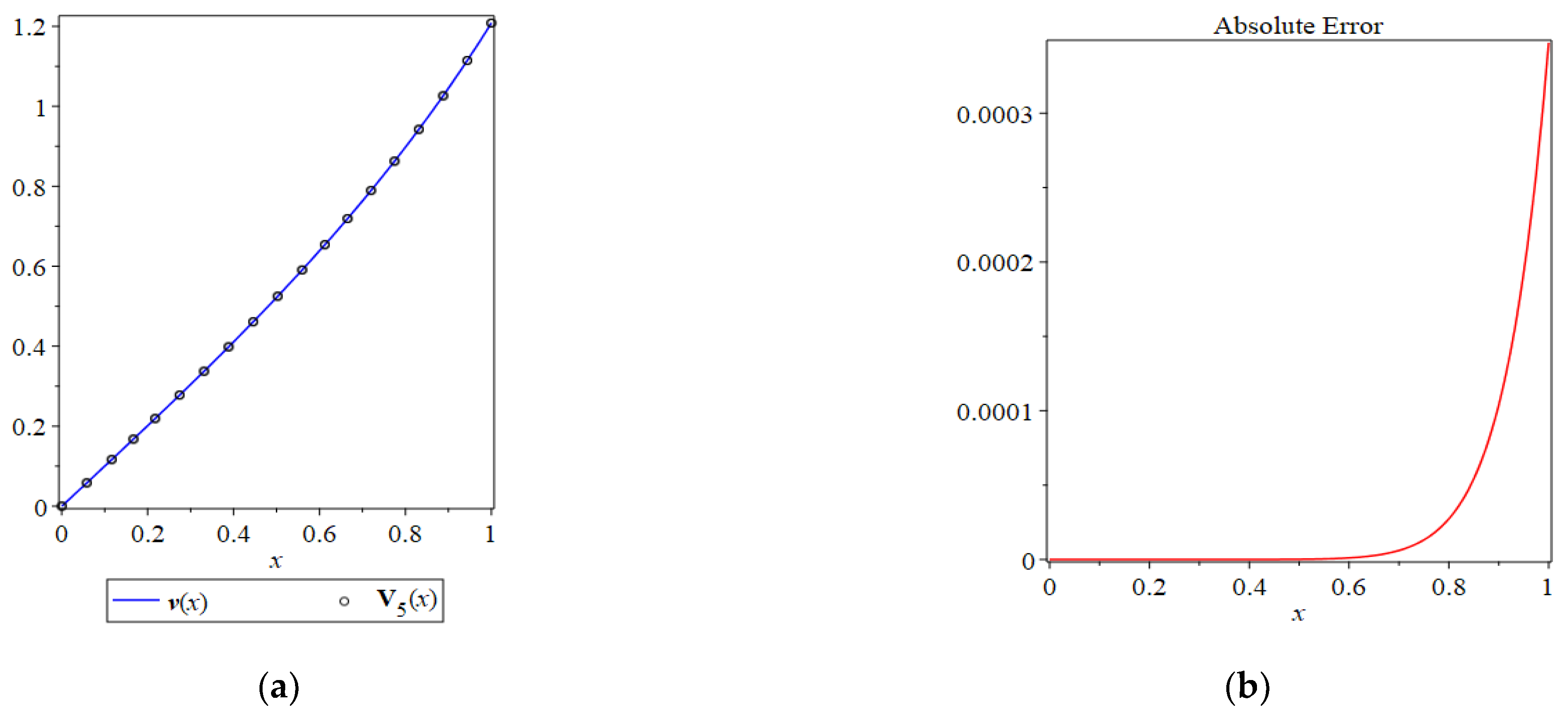
Table 2 contains a comparison between the numerical values using the truncated solution $V_5\left(x\right)$ and using the exact solution $\mathsf{\upsilon }\left(x\right)$ in the interval $x\in \left[0,1\right]$ with step size 0.1. For more clarification, the obtained series solution and the exact one were drawn together in Figure 1, as well as the absolute error between the two solutions $\left|\mathsf{\upsilon }\left(x\right) - V_5\left(x\right)\right|$.

Table 2. A comparison between the numerical results of $\mathsf{\upsilon }\left(x\right)$ and $V_5\left(x\right)$.

$\mathit{x}$	$\mathsf{\upsilon }\left(\mathit{x}\right)$	${\mathbf{V}}_5\left(\mathit{x}\right)$
0.0	0.0	0.0
0.1	0.1001670006	0.1001670007
0.2	0.2013440870	0.2013440870
0.3	0.3045825026	0.3045825023
0.4	0.4110194227	0.4110194110
0.5	0.5219305152	0.5219303730
0.6	0.6387957040	0.6387946203
0.7	0.7633858019	0.7633797217
0.8	0.8978815369	0.8978542000
0.9	1.045043135	1.044939149
1.0	1.208460241	1.208112875

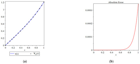
Figure 1. (a) A comparison between the exact solution $\mathsf{\upsilon }\left(x\right)$ and the series solution $V_5\left(x\right)$; (b) absolute error $\left|\mathsf{\upsilon }\left(x\right)-V_5\left(x\right)\right|$.

From Figure 1 and Table 2, it is clear that the results obtained from the HPM were in excellent agreement with the exact solution of the considered problem.

Remark. 

It is obvious that the five-term approximate solution $V_5\left(x\right)$ of the HPM was exactly the truncated Taylor series expansion of the exact solution in Equation (28) around x = 0.

• Fourth-order NIDE

As a second example, we considered the fourth-order NIDE [29]:

$${\mathsf{\upsilon }}^{(\mathrm{iv})}\left(x\right)=1+{\displaystyle \underset{0}{\overset{x}{\int }}{\mathrm{e}}^{-y}{\mathsf{\upsilon }}^2\left(y\right)}\mathrm{d}y,$$

(29)

for $x\in \left[0,1\right]$ with the following boundary conditions:

$$\begin{array}{l}\mathsf{\upsilon }\left(0\right)=1,\hspace{1em}\hspace{1em}{\mathsf{\upsilon }}^{\prime }\left(0\right)=1,\\ \mathsf{\upsilon }\left(1\right)=\mathrm{e},\hspace{1em}\hspace{1em}{\mathsf{\upsilon }}^{\prime }\left(1\right)= \mathrm{e}.\end{array}$$

(30)

Using a similar operation as illustrated in the previous example, we could write the homotopy equation as

$$\mathbf{H}\left(\mathsf{\psi },s\right)=\left(1-s\right)\left[{\mathsf{\psi }}^{(\mathrm{iv})}\left(x\right)\right]+s\left[{\mathsf{\psi }}^{(\mathrm{iv})}\left(x\right) -{\displaystyle \underset{0}{\overset{x}{\int }}{\mathrm{e}}^{-y}}{\mathsf{\psi }}^2\left(y\right)\mathrm{d}y\right]=1,s\in [0,1],x\in \left[0,1\right].$$

(31)

To simplify the integration process in the homotopy (31), we expanded ${\mathrm{e}}^{-y}$ in terms of the first five terms of the Maclaurin series, i.e., ${\mathrm{e}}^{-y}=1-y+\left(\frac{1}{2!}\right)y^2- \left(\frac{1}{3!}\right)y^3+\left(\frac{1}{4!}\right)y^4$. Therefore, substituting the solution $\mathsf{\psi }={\displaystyle \sum _{n=0}^{\infty }{s}^n{\mathsf{\psi }}_n\left(x\right)}$ into the homotopy in Equation (31) and equating the identical terms with respect to the powers of s yielded

$$\begin{array}{l}{s}^0:{\mathsf{\psi }}_0^{(\mathrm{iv})}\left(x\right)=1,\\ s^1:{\mathsf{\psi }}_1^{(\mathrm{iv})}\left(x\right)={\displaystyle \underset{0}{\overset{x}{\int }}\left(1-y+\left(\frac{1}{2!}\right)y^2-\left(\frac{1}{3!}\right)y^3+\left(\frac{1}{4!}\right)y^4\right)\left({\mathsf{\psi }}_0^2\left(y\right)\right)}\mathrm{d}y,\\ s^2:{\mathsf{\psi }}_2^{(\mathrm{iv})}\left(x\right)={\displaystyle \underset{0}{\overset{x}{\int }}\left(1-y+\left(\frac{1}{2!}\right)y^2-\left(\frac{1}{3!}\right)y^3+\left(\frac{1}{4!}\right)y^4\right)\left(2{\mathsf{\psi }}_0\left(y\right){\mathsf{\psi }}_1\left(y\right)\right)}\mathrm{d}y,\\ s^3:{\mathsf{\psi }}_3^{(\mathrm{iv})}\left(x\right)={\displaystyle \underset{0}{\overset{x}{\int }}\left(1-y+\left(\frac{1}{2!}\right)y^2-\left(\frac{1}{3!}\right)y^3+\left(\frac{1}{4!}\right)y^4\right)\left(2{\mathsf{\psi }}_0\left(y\right){\mathsf{\psi }}_2\left(y\right)+{\mathsf{\psi }}_1^2\left(y\right)\right)}\mathrm{d}y,\\ ⋮,\end{array}$$

(32)

corresponding to the following initial conditions,

$$\begin{array}{l}{\mathsf{\psi }}_0\left(0\right)=1, {\mathsf{\psi }}_0{}^{\prime }\left(0\right)=1, {\mathsf{\psi }}_0{}^{″}\left(0\right)=\mathrm{A}, {\mathsf{\psi }}_0{}^{‴}\left(0\right)=b,\\ {\mathsf{\psi }}_n={\mathsf{\psi }}_n{}^{\prime }={\mathsf{\psi }}_n{}^{″}={\mathsf{\psi }}_n{}^{‴}=0,\mathrm{at}x=0,\mathrm{for}n=1,2,3,\dots .\end{array}$$

(33)

The proposed unknown constants a and b could be estimated using the boundary conditions in Equation (30) at x = 1 after calculating a closed analytical form to the solution. Note that ${\mathsf{\upsilon }}^{″}\left(0\right)=a$ and ${\mathsf{\upsilon }}^{‴}\left(0\right)=b$. Solving the system in Equation (32) subjected to the conditions in Equation (33) yielded

$$\begin{array}{l}{V}_3\left(x\right)=1+x+\frac{a}{2} x^2+\frac{b}{6} x^3+\frac{x^4}{24}+\frac{x^5}{120}+\frac{x^6}{720}+\left(\frac{1}{5040}+\frac{a}{2520} \right)x^7+\left(\frac{b}{\mathrm{20,160}}+\frac{1}{\mathrm{40,320}}\right)x^8\\ \hspace{1em}\hspace{1em} +\left(\frac{17}{\mathrm{181,440}} a+\frac{a^2}{\mathrm{60,480}}-\frac{37}{\mathrm{362,880}}\right)x^9+\left(\frac{b}{\mathrm{37,800}}-\frac{a}{\mathrm{15,120}}+\frac{ab}{\mathrm{181,440}}-\frac{a^2}{\mathrm{120,960}}+\frac{13}{\mathrm{302,400}}\right)x^{10}\\ \hspace{1em}\hspace{1em} +\left(\frac{b^2}{\mathrm{1,995,840}}-\frac{ab}{\mathrm{332,640}}+\frac{59}{\mathrm{3,326,400}} a-\frac{19}{\mathrm{997,920}} b-\frac{41}{\mathrm{19,958,400}}+\frac{41}{\mathrm{6,652,800}} a^2\right)x^{11}\\ \hspace{1em}\hspace{1em} +\left(\frac{ab}{\mathrm{427,680}}-\frac{19}{\mathrm{5,322,240}} a^2-\frac{b^2}{\mathrm{3,421,440}}-\frac{37}{\mathrm{15,966,720}}-\frac{17}{\mathrm{9,580,032}} a+\frac{23}{\mathrm{3,991,680}} b\right)x^{12}.\end{array}$$

(34)

It is worth pointing out that the truncated series solution $V_n,n=1,2,3,\dots$ acts as approximate series solutions of increasing accuracy as $n\to \infty$. It is natural that the accuracy can be dramatically enhanced by evaluating additional terms and, therefore, produce a more accurate approximate solution. The approximate solution must consequently fulfill the boundary conditions in Equation (30). By imposing the conditions in Equation (30) at x = 1 in the full formula of $V_3$ and solving for a and b, we obtained the following real solution as an estimation of the a and b:

$$a=1.003793260,\hspace{1em}\hspace{1em}b=0.9858875713.$$

(35)

Substituting the constants a, b into the closed formula of $V_3$ yielded an approximate series solution to the considered problem. The results of the three-term approximate solution $V_3$ are shown in Table 3. To evaluate the convergence and accuracy of the HPM solution, here we mention that the NIDE in Equation (29) subjected to the given boundary conditions had the following exact solution:

$$\mathsf{\upsilon }\left(x\right)={\mathrm{e}}^x.$$

(36)

Table 3. A comparison between the numerical results of $\mathsf{\upsilon }\left(x\right)$ and $V_3\left(x\right)$.

$\mathit{x}$	$\mathsf{\upsilon }\left(\mathit{x}\right)$	${\mathbf{V}}_3\left(\mathit{x}\right)$
0.0	1.0	1.0
0.1	1.105171	1.105187
0.2	1.221403	1.221458
0.3	1.349859	1.349964
0.4	1.491825	1.491975
0.5	1.648721	1.648900
0.6	1.822119	1.822301
0.7	2.013753	2.013907
0.8	2.225541	2.225641
0.9	2.459603	2.459639
1.0	2.718282	2.718285

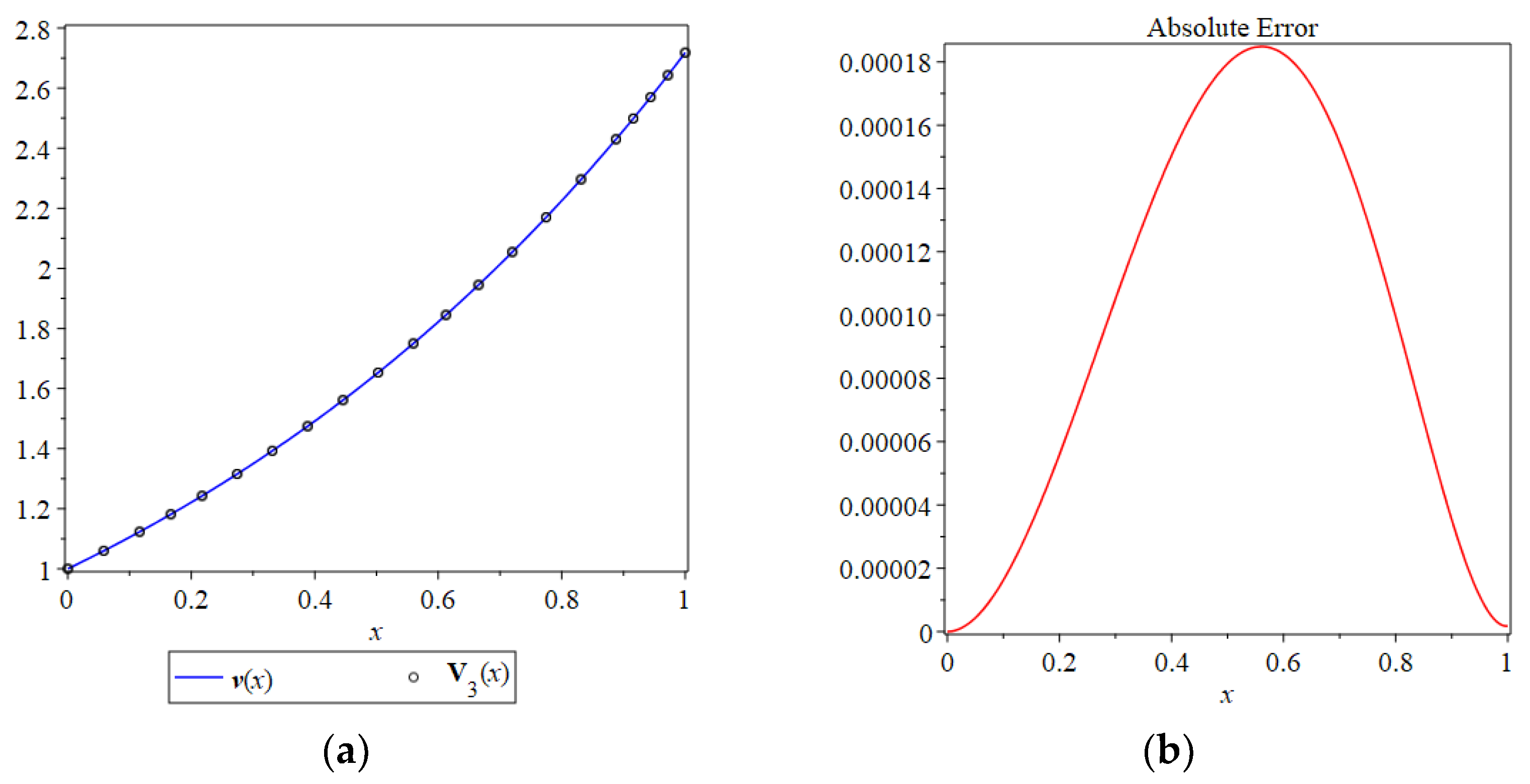
Table 3 contains a comparison between numerical values using the truncated solution $V_3\left(x\right)$ and using the exact solution $\mathsf{\upsilon }\left(x\right)={\mathrm{e}}^x$ in the interval $x\in \left[0,1\right]$ with a step size of 0.1. For more visualization, the obtained approximate solution and the exact solution were drawn together in Figure 2, as well as the absolute error between the two solutions $\left|\mathsf{\upsilon }\left(x\right)-V_3\left(x\right)\right|$. From the results presented in Figure 2 and Table 3, one can see that the obtained results of the HPM were in excellent agreement with the given exact solution.

Figure 2. (a) A comparison between the exact solution $\mathsf{\upsilon }\left(x\right)$ and the series solution $V_3\left(x\right)$; (b) absolute error $\left|\mathsf{\upsilon }\left(x\right)-V_3\left(x\right)\right|$.

• Differential equations

The applicability of the considered technique can be stated for other fields, such as nonlinear differential equations. To validate this, we considered the following initial value problem associated with the scalar Burgers’ equation [31].

$$\begin{array}{l}\frac{\partial \mathsf{\upsilon }}{\partial t}+\mathsf{\upsilon }\frac{\partial \mathsf{\upsilon }}{\partial x}-\frac{{\partial }^2\mathsf{\upsilon }}{\partial x^2}=0,\hspace{1em}\hspace{1em}\left(x,t\right) \in \mathsf{\Omega }=ℝ\times \left[0,1/2\right),\\ \mathsf{\upsilon }\left(x,0\right)=2x,\end{array}$$

(37)

Based on the homotopy perturbation technique, we constructed the following homotopy:

$$\mathbf{H}\left(\mathsf{\psi },s\right)=\left(1-s\right)\left[\frac{\partial \mathsf{\psi }\left(x,t\right)}{\partial t}\right]+s\left[\frac{\partial \mathsf{\psi }\left(x,t\right)}{\partial t}+\mathsf{\psi }\left(x,t\right)\frac{\partial \mathsf{\psi }\left(x,t\right)}{\partial x}-\frac{{\partial }^2\mathsf{\psi }\left(x,t\right)}{\partial x^2}\right]=0, s\in [0,1],x\in ℝ.$$

(38)

Substituting the solution

$$\mathsf{\psi }={\displaystyle \sum _{n=0}^{\infty }{s}^n{\mathsf{\psi }}_n\left(x,t\right)}$$

(39)

into the homotopy in Equation (38) and equating the identical terms with respect to the powers of s yielded

$$\begin{array}{l}{s}^0: \frac{\partial {\mathsf{\psi }}_1}{\partial t}=0,{\mathsf{\psi }}_0\left(x,0\right) =2x\hspace{1em}\hspace{1em}\hspace{1em}\hspace{1em}\hspace{1em}\hspace{1em}\hspace{1em}\hspace{1em}\hspace{1em}\hspace{1em}\hspace{1em}\hspace{1em}\hspace{1em}\hspace{1em}\hspace{1em}\hspace{1em}\hspace{1em} \Rightarrow {\mathsf{\psi }}_0\left(x,t\right) =2x,\\ s^1:\frac{\partial {\mathsf{\psi }}_1}{\partial t}+{\mathsf{\psi }}_0\frac{\partial {\mathsf{\psi }}_0}{\partial x}-\frac{{\partial }^2{\mathsf{\psi }}_0}{\partial x^2}=0,{\mathsf{\psi }}_1\left(x,0\right) =0\hspace{1em}\hspace{1em}\hspace{1em}\hspace{1em}\hspace{1em}\hspace{1em}\hspace{1em}\hspace{1em}\hspace{1em}\hspace{1em}\hspace{1em}\hspace{1em} \Rightarrow {\mathsf{\psi }}_1\left(x,t\right) =-4xt,\\ s^2:\frac{\partial {\mathsf{\psi }}_2}{\partial t}+{\mathsf{\psi }}_1\frac{\partial {\mathsf{\psi }}_0}{\partial x}+{\mathsf{\psi }}_0\frac{\partial {\mathsf{\psi }}_1}{\partial x}-\frac{{\partial }^2{\mathsf{\psi }}_1}{\partial x^2}=0,{\mathsf{\psi }}_2\left(x,0\right) =0\hspace{1em}\hspace{1em}\hspace{1em}\hspace{1em}\hspace{1em}\hspace{1em}\hspace{1em}\hspace{1em}\hspace{1em} \Rightarrow {\mathsf{\psi }}_2\left(x,t\right) =8x{t}^2,\\ s^3:\frac{\partial {\mathsf{\psi }}_3}{\partial t}+{\mathsf{\psi }}_0\frac{\partial {\mathsf{\psi }}_2}{\partial x}+{\mathsf{\psi }}_1\frac{\partial {\mathsf{\psi }}_1}{\partial x}+{\mathsf{\psi }}_2\frac{\partial {\mathsf{\psi }}_0}{\partial x}-\frac{{\partial }^2{\mathsf{\psi }}_2}{\partial x^2}=0,{\mathsf{\psi }}_3\left(x,0\right) =0,\hspace{1em}\hspace{1em}\hspace{1em}\hspace{1em}\hspace{1em}\hspace{1em}\Rightarrow {\mathsf{\psi }}_3\left(x,t\right) =-16x{t}^3,\\ ⋮,\\ s^n:\frac{\partial {\mathsf{\psi }}_n}{\partial t}+{\displaystyle \sum _{k=0}^{n-1}{\mathsf{\psi }}_k\frac{\partial {\mathsf{\psi }}_{n-k-1}}{\partial x}}-\frac{{\partial }^2{\mathsf{\psi }}_{n-1}}{\partial x^2}=0,n=4, 5, 6, \dots ,=0,{\mathsf{\psi }}_n\left(x,0\right) =0, \Rightarrow {\mathsf{\psi }}_n\left(x,t\right) ={\left(-1\right)}^n{2}^{n+1}x{t}^n.\end{array}$$

(40)

Hence, the (n + 1) term’s approximate solution $S_n$ could be written in the following form:

$$V_n={\displaystyle \sum _{k=0}^n{\mathsf{\psi }}_k}=2x\left(1-2t+4t^2-8t^3+\dots +{\left(-1\right)}^n{2}^n{t}^n\right).$$

(41)

Consequently from Equation (41), the exact solution of Equation (37) could be recognized as

$$\mathsf{\upsilon }\left(x,t\right)=\frac{2x}{1+2t},\left(x,t\right) \in ℝ\times \left[0,1/2\right).$$

(42)

6. Conclusions

In this work, a new formulation of the homotopy perturbation method was introduced and applied to solve several types of nonlinear integral, integro-differential and differential equations. Numerical results were displayed to demonstrate the efficiency of the newly formulated HPM. From the obtained numerical results, it is clear that the method offered highly accurate series solutions for such nonlinear integral, integro-differential and differential equations as a convergent series with terms that were easily evaluated. The proposed theorems for the convergence and for estimating the error of the HPM approximate solution validated the obtained numerical results.

References

- Mousaa, M.M.; Ragab, S.F. Application of the homotopy perturbation method to linear and nonlinear schrödinger equations. Z. Für Nat. A 2008, 63, 140–144. [Google Scholar] [CrossRef] [Green Version]
- Mousa, M.M.; Kaltayev, A. Application of the homotopy perturbation method to a magneto-elastico-viscous fluid along a semi-infinite plate. Int. J. Nonlinear Sci. Numer. Simul. 2009, 10, 1113–1120. [Google Scholar] [CrossRef]
- Barman, H.K.; Seadawy, A.R.; Akbar, M.A.; Baleanu, D. Competent closed form soliton solutions to the Riemann wave equation and the Novikov-Veselov equation. Results Phys. 2020, 17, 103131. [Google Scholar] [CrossRef]
- Ma, W.-X.; Mousa, M.M.; Ali, M.R. Application of a new hybrid method for solving singular fractional Lane–Emden-type equations in astrophysics. Mod. Phys. Lett. B 2020, 34, 2050049. [Google Scholar] [CrossRef]
- Zhao, W.; Maitama, S. Beyond sumudu transform and natural transform: 𝕁-transform properties and applications. J. Appl. Anal. Comput. 2020, 10, 1223–1241. [Google Scholar] [CrossRef]
- Khalouta, A.; KADEM, A. Solutions of nonlinear time-fractional wave-like equations with variable coefficients in the form of mittag-leffler functions. Thai J. Math. 2020, 18, 411–424. [Google Scholar]
- Ziane, D.; Belgacem, R.; Bokhari, A. A new modified Adomian decomposition method for nonlinear partial differential equations. Open J. Math. Anal. 2019, 3, 81–90. [Google Scholar] [CrossRef]
- Maitama, S.; Zhao, W. New integral transform: Shehu transform a generalization of sumudu and laplace transform for solving differential equations. Int. J. Anal. Appl. 2019, 17, 167–190. [Google Scholar] [CrossRef] [Green Version]
- Maitama, S.; Zhao, W. New Laplace-type integral transform for solving steady heat-transfer problem. Therm. Sci. 2021, 25, 1–12. [Google Scholar] [CrossRef] [Green Version]
- Sharma, D.; Samra, G.S.; Singh, P. Approximate solution for fractional attractor one-dimensional Keller-Segel equations using homotopy perturbation sumudu transform method. Nonlinear Eng. 2020, 9, 370–381. [Google Scholar] [CrossRef]
- Mousa, M.M.; Kaltayev, A. Application of he’s homotopy perturbation method for solving fractional Fokker-Planck equationss. Z. Für Nat. A 2009, 64, 788–794. [Google Scholar] [CrossRef]
- Chakraverty, S.; Mahato, N.R.; Karunakar, P.; Rao, T.D. Homotopy perturbation method. In Advanced Numerical and Semi-Analytical Methods for Differential Equations; John Wiley & Sons, Inc.: Hoboken, NJ, USA, 2019; pp. 131–139. [Google Scholar]
- He, J.-H.; El-Dib, Y.O. Homotopy perturbation method for Fangzhu oscillator. J. Math. Chem. 2020, 58, 2245–2253. [Google Scholar] [CrossRef]
- Nadeem, M.; He, J.-H.; Islam, A. The homotopy perturbation method for fractional differential equations: Part 1 Mohand transform. Int. J. Numer. Methods Heat Fluid Flow 2021, in press. [Google Scholar] [CrossRef]
- Javeed, S.; Baleanu, D.; Waheed, A.; Khan, M.S.; Affan, H. Analysis of homotopy perturbation method for solving fractional order differential equations. Mathematics 2019, 7, 40. [Google Scholar] [CrossRef] [Green Version]
- Qin, Y.; Khan, A.; Ali, I.; Al-Qurashi, M.; Khan, H.; Shah, R.; Baleanu, D. An efficient analytical approach for the solution of certain fractional-order dynamical systems. Energies 2020, 13, 2725. [Google Scholar] [CrossRef]
- Harir, A.; Melliani, S.; El Harfi, H.; Chadli, L.S. Variational iteration method and differential transformation method for solving the SEIR epidemic model. Int. J. Differ. Equ. 2020, 2020, 1–7. [Google Scholar] [CrossRef]
- Bekela, A.S.; Belachew, M.T.; Wole, G.A. A numerical method using Laplace-like transform and variational theory for solving time-fractional nonlinear partial differential equations with proportional delay. Adv. Differ. Equ. 2020, 2020, 1–19. [Google Scholar] [CrossRef]
- Bokhari, A.; Baleanu, D.; Belgacem, R. Application of Shehu transform to Atangana-Baleanu derivatives. J. Math. Comput. Sci. 2019, 20, 101–107. [Google Scholar] [CrossRef] [Green Version]
- Khan, H.; Farooq, U.; Shah, R.; Baleanu, D.; Kumam, P.; Arif, M. Analytical solutions of (2+time fractional order) dimensional physical models, using modified decomposition method. Appl. Sci. 2019, 10, 122. [Google Scholar] [CrossRef] [Green Version]
- Abuasad, S.; Hashim, I.; Karim, S.A.A. Modified fractional reduced differential transform method for the solution of multiterm time-fractional diffusion equations. Adv. Math. Phys. 2019, 2019, 1–14. [Google Scholar] [CrossRef]
- Mousa, M.M.; Ma, W.-X. A conservative numerical scheme for capturing interactions of optical solitons in a 2D coupled nonlinear Schrödinger system. Indian J. Phys. 2021, 1–11. [Google Scholar] [CrossRef]
- Mousa, M.M.; Agarwal, P.; Alsharari, F.; Momani, S. Capturing of solitons collisions and reflections in nonlinear Schrödinger type equations by a conservative scheme based on MOL. Adv. Differ. Equ. 2021, 2021, 1–15. [Google Scholar] [CrossRef]
- Lusternik, L.A. Some issues of nonlinear functional analysis. Russ. Math. Surv. 1956, 6, 145–168. [Google Scholar]
- Sidorov, N.A. Irkutsk State University The role of a priori estimates in the method of non-local continuation of solution by parameter. Bull. Irkutsk. State Univ. Ser. Math. 2020, 34, 67–76. [Google Scholar] [CrossRef]
- Noeiaghdam, S.; Dreglea, A.; He, J.; Avazzadeh, Z.; Suleman, M.; Araghi, M.A.F.; Sidorov, D.N.; Sidorov, N. Error estimation of the homotopy perturbation method to solve second kind volterra integral equations with piecewise smooth kernels: Application of the CADNA library. Symmetry 2020, 12, 1730. [Google Scholar] [CrossRef]
- Sidorov, D.N. Existence and blow-up of Kantorovich principal continuous solutions of nonlinear integral equations. Differ. Equ. 2014, 50, 1217–1224. [Google Scholar] [CrossRef]
- Adams, P.; Smith, K.; Výborný, R. Introduction to Mathematics with Maple; World Scientific Publishing Company: Singapore, 2004. [Google Scholar] [CrossRef] [Green Version]
- Polyanin, P.; Manzhirov, A.V. Handbook of Integral Equations; Chapman and Hall/CRC: Boca Raton, FL, USA, 2008. [Google Scholar]
- Avudainayagam, A.; Vani, C. Wavelet–Galerkin method for integro–differential equations. Appl. Numer. Math. 2000, 32, 247–254. [Google Scholar] [CrossRef]
- Gorguis, A. A comparison between Cole–Hopf transformation and the decomposition method for solving Burgers’ equations. Appl. Math. Comput. 2005, 173, 126–136. [Google Scholar] [CrossRef]
Publisher’s Note: MDPI stays neutral with regard to jurisdictional claims in published maps and institutional affiliations. |
© 2021 by the authors. Licensee MDPI, Basel, Switzerland. This article is an open access article distributed under the terms and conditions of the Creative Commons Attribution (CC BY) license (https://creativecommons.org/licenses/by/4.0/).