Abstract
This work proposes a new algorithm for optimizing hyper-parameters of a machine learning algorithm, RHOASo, based on conditional optimization of concave asymptotic functions. A comparative analysis of the algorithm is presented, giving particular emphasis to two important properties: the capability of the algorithm to work efficiently with a small part of a dataset and to finish the tuning process automatically, that is, without making explicit, by the user, the number of iterations that the algorithm must perform. Statistical analyses over 16 public benchmark datasets comparing the performance of seven hyper-parameter optimization algorithms with RHOASo were carried out. The efficiency of RHOASo presents the positive statistically significant differences concerning the other hyper-parameter optimization algorithms considered in the experiments. Furthermore, it is shown that, on average, the algorithm needs around of the iterations needed by other algorithms to achieve competitive performance. The results show that the algorithm presents significant stability regarding the size of the used dataset partition.
1. Introduction
Tuning the hyper-parameter configuration of a machine learning (ML) algorithm is a recommended procedure to obtain a successful ML model for a given problem. Different ML algorithms have specific hyper-parameters whose configuration requires a deep understanding of both the model and the task. Since the hyper-parameter configuration greatly impacts the models’ performance, the research in automatic hyper-parameter optimization (HPO) is focused on developing techniques that efficiently find optimal values for the hyper-parameters, maximizing accuracy while avoiding complex and expensive operations. However, this process remains a challenge because not all optimization methods are always suitable for a given problem.
Although there are several methods for tuning both continuous and discrete hyper-parameters, they do not perform equally for all ML algorithms, displaying different consumption of computational resources and stability. The process becomes computationally expensive if too many function evaluations of hyper-parameter values must be carried out to obtain a suitable accuracy. Since the size of the dataset in the HPO phase influences the dynamic complexity of the classifier but not its accuracy [1], another possible limitation is that a HPO algorithm may require a large dataset to work efficiently. Finally, most HPO algorithms are iterative, which suggests that stopping the algorithm when the expected improvement of testing new configurations is low can be a good option [2]. Nevertheless, the ML user does not have information about the rate of convergence and the loss function values. Therefore, the user usually tends to leave the default parameters (more than 50 iterations) or set a high number of iterations to assure good performance ([3]). This fact implies that the algorithm may perform more iterations than needed to obtain an adequate accuracy, with the consequent increased computational cost.
This article proposes a novel early stop HPO algorithm, RHOASo (RIASC hyper-optimization automatic software). The work aims to analyze RHOASo, compare its behavior with different state-of-the-art HPO algorithms, and measure its early-stop feature, which entails minimal human intervention.
The research questions that will be studied regarding this new algorithm are the following:
RQ1: Given a dataset, how good is the performance (accuracy, time complexity, sensibility, and specificity) of a ML algorithm when RHOASo is applied?
RQ2: How many iterations does the algorithm need until it stops? How much faster or slower is RHOASo, compared with the other HPO algorithms?
RQ3: Are there statistically meaningful differences between the performance of RHOASo and other HPO algorithms?
RQ4: Are the above results consistent? That is, do they hold for different HPO algorithms and different datasets with different characteristics (size, number of features, etc.)?
In order to test the behavior of RHOASo and answer the above questions, we have evaluated the efficiency of the algorithm combined with three well-known classifier algorithms: random forest (RF), gradient boosting (GB), and multi-layer perceptron (MLP). We choose these three supervised models because each follows a different learning paradigm: RF and GB are ensemble models (bagging and boosting models), and MLP is a type of neural network. Therefore, it is possible to study whether a particular type of model works better with the application of RHOASo.
We have measured the efficiency of RHOASo, by itself and carrying out statistical inference to evaluate how well it performs compared with the other seven HPO algorithms from several families (decision theoretic approaches, Bayesian optimization, evolutionary strategies, etc). The variables considered in the article are the accuracy, the MCC (Matthews correlation coefficient), the time complexity of the whole optimization (from initialization to termination), the sensibility, and the specificity of the obtained models. These variables are collected by applying HPOs over 16 well-known public datasets. Furthermore, the algorithm’s performances are studied by working with four different size partitions of each dataset to study their impact on the optimization performance. All of these comparisons are studied through two experiments: (a) Experiment 1 in which RHOASo carries out the number of iterations that it needs until it stops, and the other HPOs have a default input (50 iterations); and (b) Experiment 2 in which the other HPOs perform the same number of trials that RHOASo has conducted. This means that we avoid biased comparisons at the same time that we evaluate RHOASo under the default number of evaluations that a user could specify ([3]).
The results show that RHOASo works efficiently in low-dimension hyper-parameter spaces, and it is competitive in terms of accuracy and computational cost. On average, RHOASo achieves a statistically significant positive difference in terms of efficiency over 70% of the times that the algorithms are applied and obtains good results when it uses small parts of the datasets. Sensitivity and specificity also show positive results in general, although in some unbalanced datasets, there is a bias toward the majority class. Lastly, the automatic early-stop feature of RHOASo lets it finish the tuning process before reaching the fixed number of iterations given as input in the other hyper-parameter optimization methods ( vs. 50), with a 30% reduction. When fixing an equal number of iterations for all algorithms, RHOASo loses the advantage decreasing its gain to 50% on average, but remains competitive in two of the three evaluated models. It shows weakness when it is applied with MLP in some datasets.
The article is organized as follows. In Section 2, we state the hyper-parameters optimization problem when the size of the dataset is left as a variable, and we provide an overview of the state-of-the-art methods. In Section 3, we describe the proposed algorithm. First, we set and solve a conditional optimization problem for the logistic function. The solution is a simple iterative algorithm whose discrete analogous is used as the base to define RHOASo. In Section 4, we describe the experimental details of the study. Finally, in Section 5, we develop the obtained results. We analyze the performance of RHOASo when it is run together with the three ML algorithms mentioned above, and it is compared with other HPO algorithms. This is done in two different ways. On one hand, we let the number of iterations of the HPO algorithms have their default values. On the other hand, we allow the HPO algorithms to be run for the same number of iterations that RHOASo needs until it stops.
Additionally, we have included an appendix with the results concerning the first experiment in which case the ML algorithms are decision tree (DT and K-nearest neighbor (KNN). It is shown that the performance of RHOASo compared with the other HPO algorithms is substantially better. Due to the superiority of the performance of RHOASo with respect to the rest of the HPO algorithms when they are run with DT and KNN, we have carried out the complete analysis only with the RF, GB and MLP algorithms.
In order to facilitate the reading of the article, we include below a scheme describing the experimentation and validation phases that were carried out.
2. Related Work
A hyper-parameter of a ML algorithm is a hidden component that directly influences the algorithm’s behavior. Tuning it allows the user to control the performance of the algorithm.
2.1. Problem Statement
Definition 1.
Let be a tuple of random variables. Let be the space labels. Let be an i. i. d. sample whose distribution function is .
A machine learning algorithm is a functional as follows:
The model predicts the label of (unseen) instance x minimizing the expected loss function, .
This loss function measures the discrepancy between a hypothesis and an ideal predictor. The target space of functions of the algorithm, , depends on specific parameters, , that might take discrete or continuous values and have to be fixed before applying the algorithm. We use the notation to refer to the algorithm with the hyper-parameter configuration
In this scenario, another independent data set, , serves to evaluate the loss function, , provided by the algorithm ). Let the hyper-parameters remain free in .
In the case of a classification ML problem, we can take the loss function as the error rate, that is, one minus the cross-validation value. In this situation, one can define the following function:
The hyper-parameter optimization (HPO) problem consists of trying to reach
2.2. Overview of the State-of-the-Art Methods
Since the hyper-parameter configuration has a significant effect on the performance of a ML model, the main goal in the HPO research is to find optimal values for the hyper-parameters that maximize the accuracy of the model while minimizing the costs and avoiding manual tuning. In the case where hyper-parameters are continuous, HPO algorithms usually work using gradient descent-based methods ([4,5,6]) in which the search direction in the hyper-parameter space is determined by the gradient of a model selection criterion at any step.
The discrete case has several approaches that perform differently depending on the ML algorithm and the dataset. Bayesian HPO is a type of surrogate-based optimization ([7]) that tunes the hyper-parameters by keeping the assumed prior distribution of the loss function updated, taking into account the new observations that are selected by the acquisition function. The construction of this surrogate model and the hyper-parameter selection criteria result in several types of sequential model-based optimization (SMBO). The main methods model the error distribution with a Gaussian process ([8]) or tree-based algorithms, such as sequential model-based algorithm configuration (SMAC) or the Tree Parzen Estimators (TPE) method ([9,10]). Another perspective is the radial basis function optimization (RBFOpt) that proposes a deterministic surrogate model to approximate the error function of the hyper-parameters through dynamic coordinate search. These methods require fewer evaluations, improving the associated costs of Gaussian process methods ([11]). Regarding the selection function to choose the next promising hyper-parameter configuration to test in the surrogate-based optimization, the typical approach is to use the expected improvement ([8]). There are other alternatives, such as the predictive entropy search ([12]. Other variants of SMBO can be found in [13,14], where different datasets and tasks are characterized by several measurements that allow to predict a ranking of several combinations of hyper-parameter values.
Another important HPO approach is the decision-theoretic method, where the algorithm obtains the hyper-parameter setting by searching the hyper-parameter space directly following some particular strategy. As examples, we have grid search, which uses brute force, and the simple and effective random search (RS) that tests randomly sampled configurations from the hyper-parameter space [15,16]).
Other optimization algorithms are applied to the problem of discrete hyper-parameter values selection. This is the case, for instance, of the evolutionary algorithms, such as the covariance matrix adaptation evolutionary (CMA-ES) method [17], the simplex Nelder–Mead (NM) method ([18,19]) or the application of continuous techniques over the discrete case such as the particle swarm (PS) ([20,21]).
Although there are several options, these methods provide different results and consumption of computational resources, and they do not perform equally well with all ML algorithms. Then, we need to consider the costs to choose the HPO method, the size of the data required to run the optimization process effectively, and the human interaction needed. These issues arise in several open research challenges that we have summarized in Table 1.

Table 1.
Open research challenge in HPO. Content extracted from [3].
RHOASo is an HPO algorithm that is designed in order for the potential user not to have to configure the end of the process. Currently, the termination of a general HPO algorithm can be carried out in several ways ([3]): (1) an amount of runtime fixed by the user based on intuition; (2) a lower bound of the generalization error specified by the user; and (3) considering the convergence of HPO if no progress is identified. All of these procedures can lead to over-optimistic bounds or excessive runtime that increases the computational cost. In this scenario, RHOASo is able to stop automatically, without losing accuracy and with minimal intervention of the user.
Additionally, many of the state-of-the-art HPO algorithms have, in turn, parameters that must be set up before running them. For instance, when a user wants to tune an (unbounded) integer-valued hyper-parameter of a given ML algorithm, the HPO algorithm requires the user to pre-configure a grid over which it is to be run. In many cases, the higher the size of the grid, the higher the execution cost of the HPO algorithm. A natural way to proceed in these cases is to accelerate the hyper-parameter running process, using early-stopping techniques ([2,22,23,24]). However, these algorithms still have other parameters that must be set up. Therefore, in some sense, HPO algorithms move the hyper-parameter tuning problem from ML algorithms to themselves, which increases the complexity and cost of the whole process. Table 2 below shows the parameters on which the HPO algorithms used in this work depend.
Table 2.
Hyper-parameters of the HPO algorithms considered in this work.
Thus, the natural question is how to tune hyper-parameters of HPO algorithms without increasing the complexity. Since using HPO algorithms over themselves does not solve the problem, it is natural to ask for HPO algorithms depending on as few hyper-parameters as possible and achieving good performance, compared with state-of-the-art HPO algorithms.
Our aim is to present a novel HPO algorithm with only one parameter to be tuned and to analyze its performance, compared with other state-of-the-art HPO algorithms.
3. The Proposed Algorithm: RHOASo
RHOASo is an approach to the HPO problem, whose underlying idea is the reversible gradient-based HPO method proposed for the continuous case ([5]).
Open source code for RHOASo is hosted in GitHub (https://github.com/amunc/RHOASo, accessed on: 25 July 2021), and it is available under the GPL license (version 3). Users do not need to install software separately, save for the Python language. Additionally, this is included in a ML intelligent system, RADSSo (RIASC automated decision support software), and it was used in several research works ([29,30]).
3.1. The Setup
Recall from Section 2.1 that the space of functions in which a learning algorithm takes values is assumed to depend on certain parameters , and this space of functions is denoted by . We make the following assumptions:
- The hyper-parameters are discrete.
- If , then .
Typical examples of hyper-parameters satisfying such assumptions are the maximum depth in any tree-based machine learning model, the number of trees if the output of the model is a weighted average of the outputs of all the trees, or the number of neurons in hidden layers of a multilayer perceptron (the weights of the inputs of a given neuron may be zero).
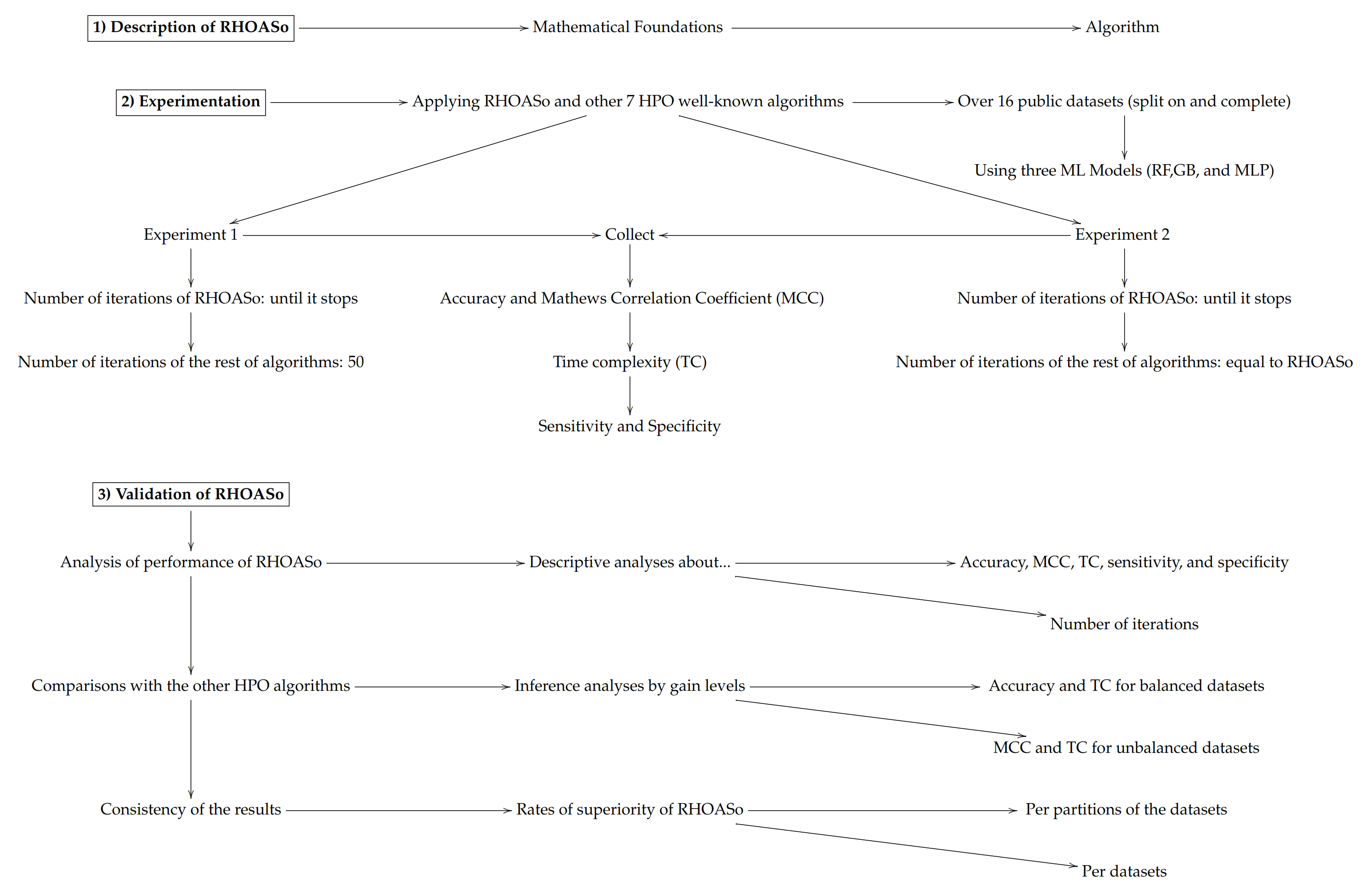
Let be the functional given in Equation (2) for a given machine learning model defined by a dataset D and a model . If we plot the functional considering, for example, the model random forest with hyper-parameters maximum depth (x-axis) and number of trees (y-axis), we can obtain a figure like those shown in Figure 1 (the plots are obtained from two different datasets).
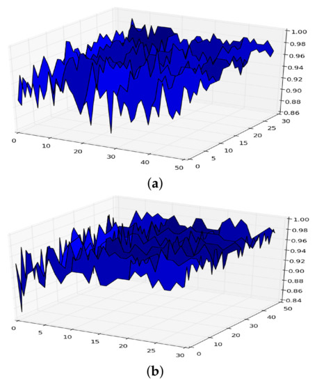
Figure 1.
Surface of for random forest. (a) in RF. (b) in RF.
From the expression it follows that if we let both the size of the dataset and the number of iterations in the cross-validation go to infinity, the surface given in Figure 1 becomes smoother, and takes the form shown in Figure 2, which is a concave surface with an asymptote in the plane .

Figure 2.
Smoothing of .
At this point, one can ask for an algorithm to find a value of at which attains a sufficiently high value while keeping and as small as possible.
3.2. Motivation of the Algorithm
In order to motivate the algorithm, consider the logistic function restricted to . This is a concave function with an asymptote in , thus it has no maximum. Although the maximization problem of this function has no sense, we can ask for the point with higher value subject to the condition that making smaller makes the decrease in f important. One way to formalize this question is by considering the maximization problem of the function . In a certain sense, maximizing consists of choosing a point with a sufficiently large image but whose slope at that point is not too low. Note that , and therefore , has only one solution, , which is a maximum.
Consider now the function , n being a natural number. Then, taking , the equation has only one solution , which is greater than , and becomes larger as we make n increase. Thus, we can control how small the slope is at the solution by making n vary.
In order to explain how RHOASo works, and to link directly with the form it is presented below, let us denote the function f by and let us restrict its domain of definition to the set of natural numbers. The variable is now denoted by . Then, instead of the derivative, we may consider the following function:
where h is a natural number. In order to simplify the notation, we set . Thus, we may consider the optimization problem defined by the following:
where
Now, we can give a simple iterative algorithm to find the value close to that at which attains a sufficiently high value while keeping the magnitude of such coordinate as low as possible; at the iteration i, do: if , then and stop otherwise. This is just the most basic algorithm to solve the optimization problem . Observe that the convergence is always ensured because of the properties of the function .
See Figure 3 to show how the stabilizer function, Stb, behaves in two particular cases.
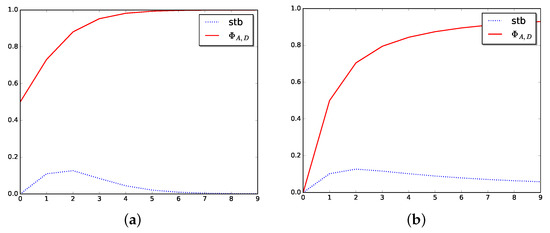
Figure 3.
Stabilizer in dimension one. (a) Stabilizer for logistic function. (b) Stabilizer for arctangent function.
3.3. The Algorithm
There are two important features we want for the algorithm to have. On one hand, we want to avoid meta-parameters, that is, we want for the algorithm not to depend (strongly) on extra parameters. In state-of-the-art HPO algorithms, the user has to set as input the exact number of iterations that the algorithm must perform. On the other hand, we want the algorithm to give a good result when it is run, giving as input not the whole dataset but a small part of it. The proposed HPO algorithm exploits the consequences derived from assumptions 1 and 2 to reach the objective in a simple way.
Since the hyper-parameters we will work with are discrete, we may assume that the hyper-parameter space is . Suppose that we are at the point of the hyper-parameter space. The decision about to which next point the algorithm must jump is based on two basic rules:
- Fix a natural number h. Let . We look at the points . These are the next points at each possible direction in the space . Since , for each , it is likely that for each , will give a better result than .
- Given , define its stabilizer as follows:If we are at point , we will transit at point if the inequality holds true and .
- Once the algorithm stops at some point , there is a final step at which the point with maximum is found and given as the final output.
The pseudo-code of the algorithm is included in Algorithms 1–4.
| Algorithm 1 Computing stabilizer. |
|
| Algorithm 2 Computing best neighbor. |
|
4. Materials and Methods
Some experiments were carried out in order to answer the research questions formulated in the introduction:
- RQ1: Given a dataset, how good is the performance (accuracy, time complexity, sensibility, and specificity) of a ML algorithm when RHOASo is applied?
Algorithm 3 Last phase. - 1:
- Input: data, train_data, test_data, features, target
- 2:
- Output: next hyper-parameters giving best accuracy
- 3:
- procedureLastPhase()
- 4:
- 5:
- 6:
- for in do
- 7:
- 8:
- 9:
- end for
- 10:
- 11:
- return maximum
- 12:
- end procedure
Algorithm 4 RHOASo algorithm. - 1:
- Input: data, train_data, test_data, features, target, max_pars
- 2:
- Output: best hyper-parameters
- 3:
- Initialize
- 4:
- while True do
- 5:
- GetStab
- 6:
- GetBestNeigh
- 7:
- if then
- 8:
- 9:
- else
- 10:
- 11:
- end if
- 12:
- end while
- 13:
- = LastPhase
- 14:
- return
- RQ2: How many iterations does the algorithm need until it stops? How much faster or slower is RHOASo, compared with the other HPO algorithms?
- RQ3: Are there statistically meaningful differences between the performance of RHOASo and other HPO algorithms?
- RQ4: Are the above results consistent? That is, do they hold for different HPO algorithms and different datasets with different characteristics (size, number of features, etc.)?
The analyses aim to measure the quality of the proposed algorithm and decide whether there are statistically meaningful differences between the performance of the selected HPO methods and RHOASo.
4.1. ML and HPO Algorithms
We have evaluated the efficiency of three well-known ML algorithms:
- RF is an ensemble classifier consisting of a set of decision trees. Each tree is constructed by applying bootstrap re-sampling (bagging) to the training set, which extracts a subset of samples for training each tree. Therefore, the trees will have a weak correlation and give independent results. In the case of RF, we have two main hyper-parameters: the number of decision trees to be used and the maximum depth for each of them ([31]).
- GB is another ensemble technique in which the predictors are made sequentially, learning from the previous predictor’s mistakes to optimize the subsequent learner. It usually takes fewer iterations to reach close-to-actual predictions, but the stopping criteria have to be chosen carefully. This technique reduces bias and variance but can induce overfitting if too much importance is assigned to the previous errors. We tune two discrete hyper-parameters: the number of predictors and their maximum depth ([32,33]).
- A MLP is a graph-type model that is organized in ordered layers (input layer, output layer, and hidden layers). Each layer consists of a set of nodes with no connections between them, so the connections occur between nodes belonging to different and contiguous layers. In this study, we set two hidden layers, and we tune the number of neurons in each of these hidden layers.
In Table 3, we give a summary of the ML algorithms we have used together with the hyper-parameters we have tuned. The search space for all hyper-parameters is in the interval [1, 50]. All hyper-parameters not being tuned are set to their default values as per scikit-learn implementation ([34]). We have used 10-fold cross-validation to assess the performance of all ML models combined with the HPO algorithms.
Table 3.
ML algorithms together with hyper-parameters we have considered.
On the other hand, in Table 4 a summary of the HPO algorithms selected for this study is given.
Table 4.
HPO algorithms used. Colors explanation: Bayesian methods in blue, decision-theoretic techniques in pink, evolutionary algorithms in brown, and other optimization algorithms in green.
4.2. Datasets
The datasets selected for the experiments are described in Table 5. The choice was motivated by different reasons: availability in public servers to verify the results, the number of instances and classes, and the type of features. There are 16 public benchmark datasets with a different number of variables (8–300), rows (4601–284,807), and classes (2–10). Since the size of the dataset in the HPO phase influences the performance of the classifier ([1]), the performances of the algorithms are analyzed with four different-sized partitions of each dataset (). These proportions are chosen because, in this way, the number of instances is in different orders of magnitude. In addition, each dataset is divided into train data (80%) and validation data (20%) , and the partitioning scheme above is applied to obtain train and validation subsets with the corresponding proportions .
Table 5.
Descriptions of datasets.
The transformation of features to obtain treatable datasets to input directly to each model is manually implemented with Python.
4.3. Construction of the Response Variables
In order to build response variables to measure the performance of the HPO algorithms, we apply them to each ML model over each partition, , obtaining a hyper-parameter configuration for . Then, the learning algorithm with the obtained hyper-parameter configuration is run over to construct a classifier that is validated over . At this step, we collect the obtained accuracy. This scenario is repeated a number of times (trials), giving rise to two different experiments.
- Experiment 1: the experimentation is repeated 50 times (trials) for all HPOs, except for RHOASo, which automatically stops when it considers that it has obtained an optimal hyper-parameter configuration.
- Experiment 2: the experimentation is repeated for all HPOs as many times (trials) as RHOASo has carried out until stopping.
The time complexity of the whole process is stored as well. The time complexity, measured in seconds, is the sum of the time needed by the HPO algorithm to find the optimal hyper-parameter configuration, and the time that the ML algorithm uses for training. Then, we create two response variables. We denote by the array where the m-th component is the accuracy of the predictive model tested on that was trained over with the hyper-parameters at the m-th trial. is the notation for time complexity.
We have also collected the sensitivity and the specificity of each iteration for RHOASo to measure its performance more accurately.
Additionally, we have collected the MCC (Matthew correlation coefficient), which is defined as follows:
where TP, TN, FP, and FN denote true positives, true negatives, false positives, and false negatives, respectively. This coefficient works as a substitute metric of the accuracy for unbalanced datasets [55,56]. Since some datasets contain a certain degree of imbalance, we present our results with both indicators, accuracy and MCC.
4.4. Statistical Analyses
Our main objective is to analyze the quality of the RHOASo algorithm and compare it with other HPO algorithms. In order to analyze whether there are meaningful statistical differences among the obtained results by the HPO algorithms and RHOASo, we perform the following statistical analysis:
- We have conducted descriptive and exploratory analyses of , , the MCC, the sensibility, and the specificity of RHOASo in order to check how well RHOASo performs the tasks.
- We have computed the average of iterations that RHOASo executes until it automatically stops.The following inference tests are carried out for both Experiments 1 and 2.
- To compare RHOASo’s efficiency with that of the other HPO algorithms, we carry out non-parametric tests, due to the non-normality of the data and . Wilcoxon’s tests for two paired samples are conducted comparing each with and with for all datasets and for the three selected ML algorithms. The choice of Wilcoxon’s test is because the response variables that we compare are obtained by the application of the ML algorithms over the same dataset but with different settings . We obtain the results at a significance level of .
- Once we apply the inference described above, we obtain the p-values of 7 comparisons along 16 datasets with 4 partitions in each one, providing a total of 448 decisions on statistical difference for each ML algorithm and for each response variable, obtaining, thus, 2688 p-values. From these results, we have computed how many times we obtain positive difference (), negative difference () or equality (), see Table 6.
Table 6. Conditions of validity. The symbols =, >, < denote statistically meaningful equality and difference, and Me denotes the median.
- Since the blue cells may be understood as being both a positive difference or negative difference, depending on the improvement that we obtain, we have reclassified the results, creating a new table, correcting these cases by the rule described in Equation (5).whereand
- We have completed the analysis by computing the rate of each type of validity (red, yellow and green cells) as follows:where N denotes the number of total possible comparisons. Since we have performed the computations for each ML algorithm, we have .
- Finally, we compute per partition and per dataset to analyze the consistency of the results.
Note that for studying the cases of unbalanced datasets, we have carried out the analyses described above by changing the accuracy for the MCC.
4.5. Technical Details
The analyses are carried out at high-performance computing over HP ProLiant SL270s Gen8 SE, with two processors, Intel Xeon CPU E5-2670 v2 @ 2.50GHz, with 10 cores each and 128 GB of RAM and one hard disk of 1 TB. The analysis script is implemented in Python language.
5. Results and Discussion
This section is organized according to the research questions we have formulated in the introduction.
5.1. Research Question 1: Given a Dataset, How Good Are the ML Models When RHOASo Is Applied?
Since the behavior of RHOASo is similar in both Experiments 1 and 2, in this section, we detail the performance of RHOASo in Experiment 1, and we include a summary of the results for Experiment 2.
5.1.1. Performance in Experiment 1
We can see in Figure 4 the median of the accuracy when RHOASo is applied. The median for RF is 0.92, for GB it is 0.9058, and for MLP it is 0.8182. We can see that in all of these cases, it is greater than 0.80. We can observe that the achieved accuracy by RHOASo presents great stability in terms of the partitions of the dataset, except for dataset with model RF, and dataset with model GB. In the case of , the variation appears when we change from to . This dataset is the largest one in the study, with the highest rate of unbalanced data. Then, the most appropriate metric is the MCC. As is discussed later, the MCC remains stable for in all the partitions. The case of is more involved. The most frequent hyper-parameter configurations that RHOASo computes for each partition are , for (14 times out of 50), , for (50 times out of 50), , for (31 times out of 50), and , for (50 times out of 50). Since the number of features in is 12, there are few instances, and the dataset is unbalanced, the most probable explanation is that the model is overfitting the training data. This behavior appears also in the rest of the metrics with the combination and GB. The stability is not as evident when the dataset changes, although the general trend is maintained through the ML models. For instance, the obtained models with provide the worst accuracy for the three ML algorithms. Although it may seem that the accuracy is not very high, the rest of the HPO does not achieve better results, as is outlined below. For this reason, the fit achieved by RHOASo is considered to be sufficient.
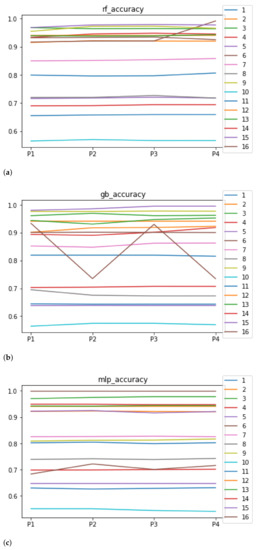
Figure 4.
Behavior of RHOASo: accuracy. Each line represents a dataset. (a) Accuracy for RF. Axis X: the partition of the dataset. Axis Y: the obtained accuracy. (b) Accuracy for GB. Axis X: the partition of the dataset. Axis Y: the obtained accuracy. (c) Accuracy for MLP. Axis X: the partition of the dataset. Axis Y: the obtained accuracy.
We can see in Figure 5 the median of the MCC () when RHOASo is applied. The median for RF is 0.51, for GB it is 0.40, and for MLP it is 0.32. The MCC value considers class imbalance, so the results worsen for accuracy, particularly in datasets 3 and 12, which are highly unbalanced: the minority classes contain less than 1% of total instances. Apart from unbalanced datasets, the trends are similar to those presented when evaluating the accuracy.
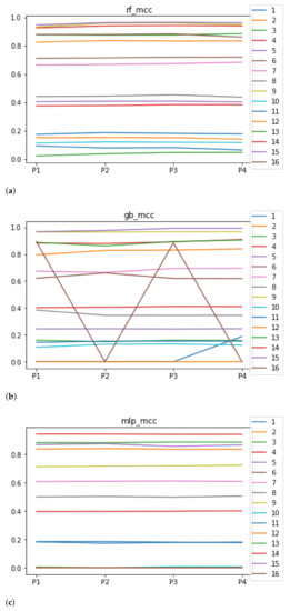
Figure 5.
Behavior of RHOASo: MCC. Each line represents a dataset. (a) MCC for RF. Axis X: the partition of the dataset. Axis Y: the obtained MCC. (b) MCC for GB. Axis X: the partition of the dataset. Axis Y: the obtained MCC. (c) MCC for MLP. Axis X: the partition of the dataset. Axis Y: the obtained MCC.
As far as the time complexity is concerned, the median results are included in Figure 6. The median value for RF is 1.3028 s, and for GB it is 4.2567 s. The MLP stands out for its high computational cost, with 259.8138 s. Regarding the stability, as expected, the larger the partition size that is used, the larger the time complexity, independently of the ML algorithm used together with RHOASo. Nevertheless, this behavior is different for each ML algorithm. It is worth noting that in the case of RF, the increase in time complexity as the size of the partitions increases is much smoother for most of the datasets, compared to GB and MLP.
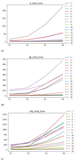
Figure 6.
Behavior of RHOASo: time complexity. Each line represents a dataset. (a) Time complexity for RF. Axis X: the partition of the dataset. Axis Y: the obtained time complexity in seconds. (b) Time complexity for GB. Axis X: the partition of the dataset. Axis Y: the obtained time complexity in seconds. (c) Time complexity for MLP. Axis X: the partition of the dataset. Axis Y: the obtained time complexity in seconds.
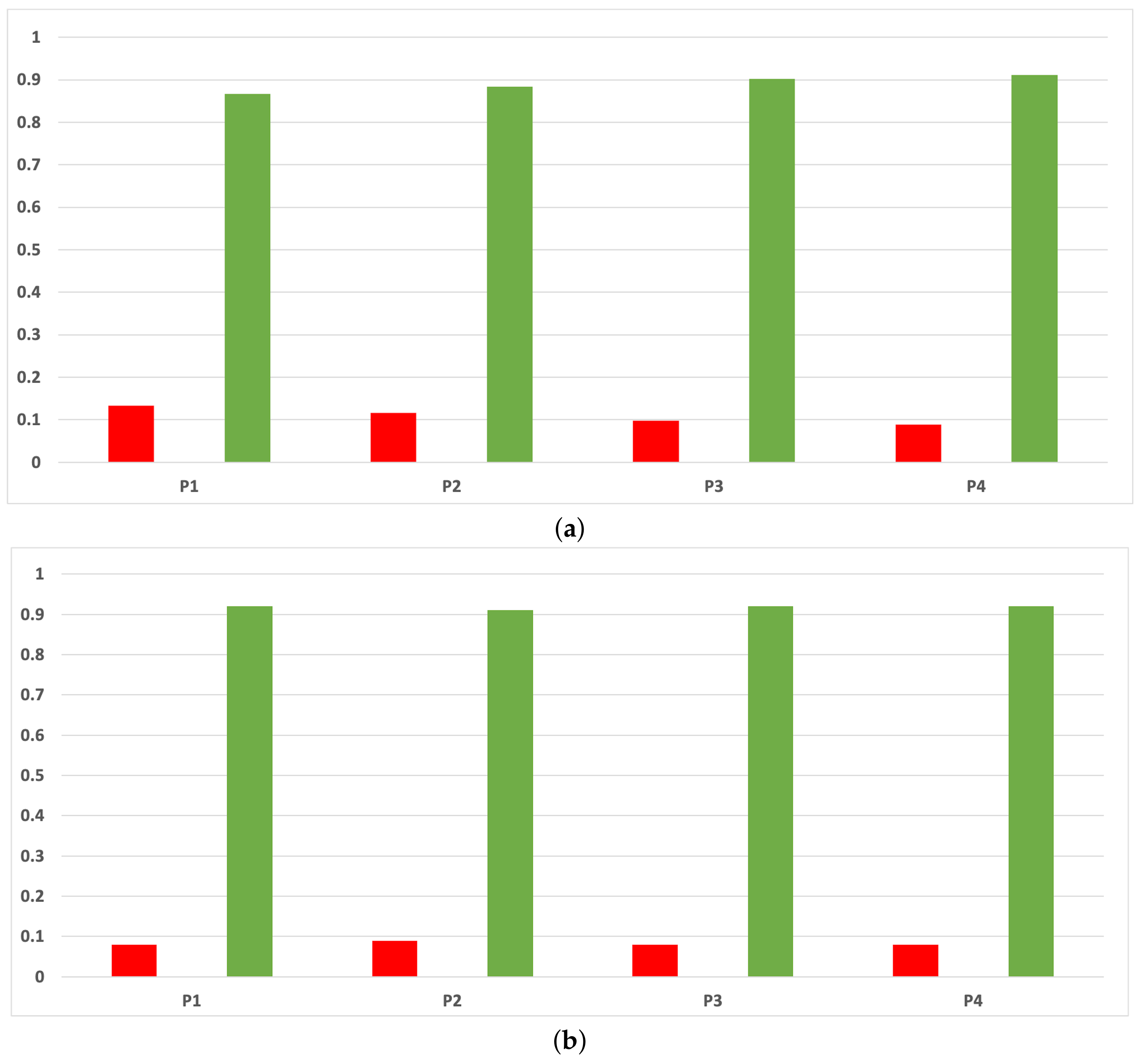
Sensitivity and specificity are plotted in Figure 7 and Figure 8. The results are stable across partitions and datasets, which achieve similar results, even when using different models, except for and GB. The median of sensitivity is 0.9 for GB, 0.91 for MLP, and 0.88 for RF. In contrast, specificity has a median of 0.7 for GB, 0.69 for MLP, and 0.733 for RF. The lower specificity could be caused by the imbalance between classes in specific datasets (see Table 5), which causes the models to be biased toward the majority class. However, has both low specificity and low sensitivity. Overall, the trends are similar to those found in the evaluation of accuracy.
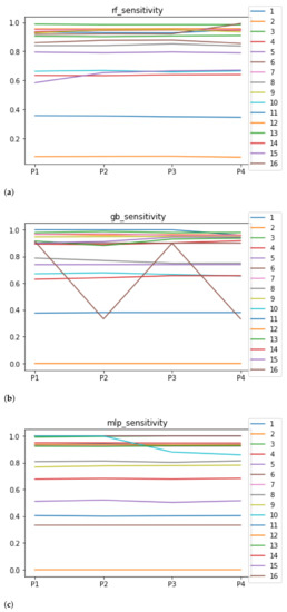
Figure 7.
Behavior RHOASo: sensitivity. The datasets are represented with a bar chart for each partition. (a) Sensitivity for RF. Axis X: the partition of the dataset. Axis Y: the obtained sensitivity. (b) Sensitivity for GB. Axis X: the partition of the dataset. Axis Y: the obtained sensitivity. (c) Sensitivity for MLP. Axis X: the partition of the dataset. Axis Y: the obtained sensitivity.
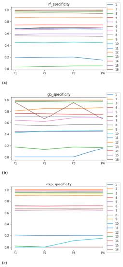
Figure 8.
Behavior RHOASo: specificity. The datasets are represented with a bar chart for each partition. (a) Specificity for RF. Axis X: the partition of the dataset. Axis Y: the obtained specificity. (b) Specificity for GB. Axis X: the partition of the dataset. Axis Y: the obtained specificity. (c) Specificity for MLP. Axis X: the partition of the dataset. Axis Y: the obtained specificity.
5.1.2. Performance in Experiment 2
Since the behavior of RHOASo in both experiments is the same, we include in Table 7 a summary with the median of all metrics (without taking into account partitions) that RHOASo has obtained in Experiment 2.
Table 7.
Medians of response variables for RHOASo in Experiment 2.
5.2. Research Question 2: How Many Iterations Does the Algorithm Need until It Stops? How Faster or Slower Is RHOASo Compared with the Other HPO Algorithms?
The number of iterations that RHOASo has needed until stopping for Experiment 1 is included in Figure 9. In the case of Experiment 2, this information can be observed in Table 7.
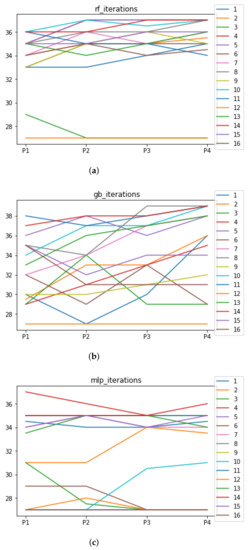
Figure 9.
Number of iterations per partition. Each line represents a dataset (medians). (a) Number of iterations RF. In axis X, the partition of the dataset. In axis Y, the number of the iterations that RHOASo has carried out. (b) Number of iterations GB. In axis X, the partition of the dataset. In axis Y, the number of the iterations that RHOASo has carried out. (c) Number of iterations MLP. In axis X, the partition of the dataset. In axis Y, the number of the iterations that RHOASo has carried out.
In Experiment 1, we can see the median of the number of iterations needed by RHOASo for each ML algorithm, each dataset and each partition. As general result, the median of the number of iterations for each partition (computed over all datasets) is 35 for RF, 33.5 for GB, and 34 iterations for MLP. Taking into account that the number of iterations given as input (by default) in the rest of HPO algorithms is equal to 50, it implies that, on average, RHOASo needs approximately of the iterations required by the other algorithms. Additionally, it stops the process by itself. As a consequence of this fact, less time is required by RHOASo to obtain a good enough accuracy and is able to be more competitive than other algorithms. This is most significant in the case of MLP, where each iteration is highly resource consuming. There is not a clear trend relating the partition size and number of iterations, especially in the case of GB, in which there is a greater variability in the number of iterations. It could be expected that a greater amount of data would contribute to a faster convergence, but this is not case. Therefore, it is likely that the functional may not be as concave, as it would be desirable to perform an effective early stopping.
We have not compared whether RHOASo is faster or slower, compared with the other HPO algorithms for Experiment 2 by the very nature of the design of the experiment.
5.3. Research Question 3: Are There Statistically Meaningful Differences between the Performance of RHOASo and the Other HPO Algorithms?
We remind that we have carried out two experiments:
- Experiment 1: the experimentation is repeated 50 times (trials) for all HPOs except for RHOASo, which automatically stops when it considers that it has obtained an optimal hyper-parameter configuration.
- Experiment 2: the experimentation is repeated for all HPOs as many times (trials) as RHOASo has carried out until stopping.
5.3.1. Experiment 1
In Figure 10 and Figure 11, the performances (accuracies and time complexities) that are achieved by the HPO algorithms over each dataset are shown.
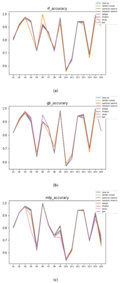
Figure 10.
Accuracy complexity. (a) Accuracy in RF. In axis X, the dataset. In axis Y, the accuracy obtained. Each line represents a HPO algorithm. (b) Accuracy in GB. In axis X, the dataset. In axis Y, the accuracy obtained. Each line represents a HPO algorithm. (c) Accuracy in MLP. In axis X, the dataset. In axis Y, the accuracy obtained. Each line represents a HPO algorithm.

Figure 11.
Time complexity. (a) Time complexity in RF. In axis X, the dataset. In axis Y, the total time obtained measured in seconds. Each line represents a HPO algorithm. (b) Time complexity in GB. In axis X, the dataset. In axis Y, the total time obtained measured in seconds. Each line represents a HPO algorithm. (c) Time complexity in MLP. In axis X, the dataset. In axis Y, the total time obtained measured in seconds. Each line represents a HPO algorithm.
However, if we want to compare whether RHOASo obtains any gain against the other HPO algorithms, we need to carry out more detailed analyses. This is the study of the validity of RHOASo.
The rates of validity that are obtained by RHOASo, compared to the rest of the HPO algorithms are included in Table 8. Note that these computations are carried out with the accuracies and time complexities by the analyses that are explained in Section 4.4.
Table 8.
Rate of validity of RHOASo vs. HPO across all (% with accuracy and time complexity).
On average, the class corresponding to positive statistically significative differences (green class) is higher than . This can be considered a good result since RHOASo achieves better results than the rest of the algorithms in more than half of the cases analyzed. However, there is still a high rate in the blue class. Once we have transformed the blue class (see Section 4.4), we can analyze whether RHOASo is more effective than the rest of the HPO algorithms. The results are included in Table 9, which show that, on average, the class corresponding to positive statistically significative differences is higher than .
Table 9.
Rate of validity of RHOASo vs. HPO across all (% with accuracy and time complexity).
After confirming that RHOASo is 70% more efficient than the rest of the HPO algorithms, the question that arises is whether there is a pattern in the 30% of the cases in which it does not succeed. For example, it might be possible for RHOASo to fail for datasets with a certain dimensionality, or for a specific ML algorithm. Another possibility is that RHOASo always loses against the same HPO algorithm. For this reason, we are going to study in depth the consistency of the previous results.
Since we have dealt with unbalanced datasets, such as or , we have repeated the analyses, changing the metric of accuracy by MCC so as to avoid over-optimistic scores. In Figure 12, the MCCs that are achieved by the HPO algorithms over each dataset are shown.
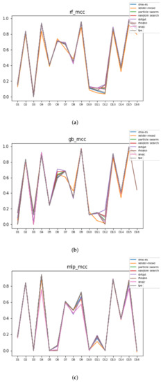
Figure 12.
MCC of all HPO algorithms. (a) MCC in RF. In axis X, the dataset. In axis Y, the MCC obtained. Each line represents a HPO algorithm. (b) MCC in GB. In axis X, the dataset. In axis Y, the MCC obtained. Each line represents a HPO algorithm. (c) MCC in MLP. In axis X, the dataset. In axis Y, the MCC obtained. Each line represents a HPO algorithm.
The rates of validity that are obtained by RHOASo, compared to the rest of the HPO algorithms, are included in Table 10. Note that these computations are carried out with the MCCs and time complexities by the analyses that are explained in Section 4.4.
Table 10.
Rate of validity of RHOASo vs. HPO across all (% with MCC and time complexity).
We can observe that RHOASo maintains its rate of gain, overcoming 70% of the cases. In Section 5.4, we study the consistency of these results as well as those situations in which RHOASo does not obtain a gain.
5.3.2. Experiment 2
In Figure 13 and Figure 14, the performances (accuracies and time complexities) that are achieved by the HPO algorithms over each dataset are shown.
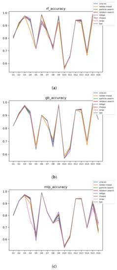
Figure 13.
Experiment 2: Accuracy complexity. (a) Accuracy in RF. In axis X, the dataset. In axis Y, the accuracy obtained. Each line represents a HPO algorithm. (b) Accuracy in GB. In axis X, the dataset. In axis Y, the accuracy obtained. Each line represents a HPO algorithm. (c) Accuracy in MLP. In axis X, the dataset. In axis Y, the accuracy obtained. Each line represents a HPO algorithm.
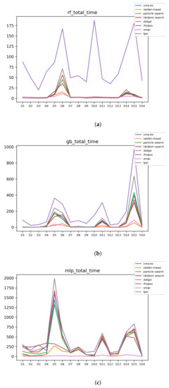
Figure 14.
Experiment 2: Time complexity. (a) Time complexity in RF. In axis X, the dataset. In axis Y, the total time obtained measured in seconds. Each line represents a HPO algorithm. (b) Time complexity in GB. In axis X, the dataset. In axis Y, the total time obtained measured in seconds. Each line represents a HPO algorithm. (c) Time complexity in MLP. In axis X, the dataset. In axis Y, the total time obtained measured in seconds. Each line represents a HPO algorithm.
The rates of validity that have been obtained by RHOASo compared to the rest of HPO of algorithms are included in Table 11. Note that these computations are carried out with the accuracies and time complexities by the analyses that are explained in Section 4.4 for Experiment 2.
Table 11.
Experiment 2: Rate of validity of RHOASo vs. HPO across all (% with accuracy and time complexity).
In this experiment, RHOASo loses some of its advantage over other HPO algorithms, mainly because the improvement in execution time is lower since the number of iterations of the other algorithms is fixed to be equal to that of RHOASo. The average gain is of 53.86%, which is lower than the 71.96% obtained when evaluating the accuracy. Nevertheless, RHOASo performs better for GB, has a slight advantage for RF and is outperformed in MLP. This fact may be related to the search strategy of RHOASo. MLP has worse performance than other models across all datasets and configurations, which increases the number of neurons that tend to perform better, but the search strategy of RHOASo favors configurations with low magnitude of hyper-parameter values. Therefore, the performance when tuning MLP can be expected to be less satisfactory.
For the unbalanced datasets, we have included the analyses changing the metric of accuracy by MCC. In Figure 15, the MCCs that are achieved by the HPO algorithms over each dataset are shown.
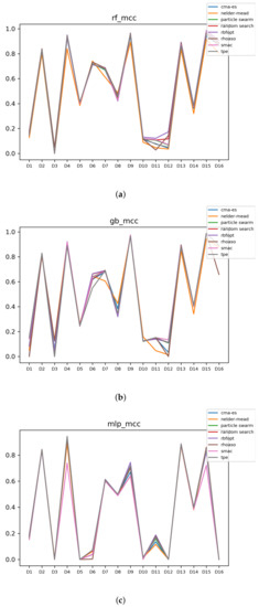
Figure 15.
Experiment 2: MCC of all HPO algorithms. (a) MCC in RF. In axis X, the dataset. In axis Y, the MCC obtained. Each line represents a HPO algorithm. (b) MCC in GB. In axis X, the dataset. In axis Y, the MCC obtained. Each line represents a HPO algorithm. (c) MCC in MLP. In axis X, the dataset. In axis Y, the MCC obtained. Each line represents a HPO algorithm.
The rates of validity that are obtained by RHOASo, compared to the rest of HPO of algorithms are included in Table 12. Note that these computations are carried out with the MCCs and time complexities by the analyses that are explained in Section 4.4.
Table 12.
Experiment 2: rate of validity of RHOASo Vs HPO across all (% with MCC and time complexity).
When using MCC as the reference metric, the results follow similar trends to that of accuracy. RHOASo gains a slight advantage for RF and incurs a slight loss for MLP, but there are no significant differences.
5.4. Research Question 4: Are the above Results Consistent?
In this section, we analyze whether RHOASo achieves a significant performance improvement consistently across datasets and partitions.
5.4.1. Experiment 1
The rates of validity for each partition computed with the accuracy and time complexity are included in Figure 16. The consistency of the green class is clear when we discriminate them by partitions. That is to say, if we only consider the partitions, RHOASo always outperforms the rest of the HPO algorithms. This may be due to the early stop of RHOASo, consuming less time but achieving good accuracy.
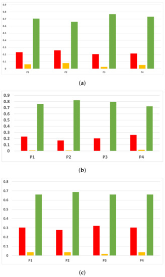
Figure 16.
Experiment 1: consistency per partition (accuracy and time complexity). (a) Rate of validity per partition in RF. In axis X, the partition of the dataset. In axis Y, the rate of RHOASo for each class of validity. (b) Rate of validity per partition in GB. In axis X, the partition of the dataset. In axis Y, the rate of RHOASo for each class of validity. (c) Rate of validity per partition in MLP. In axis X, the partition of the dataset. In axis Y, the rate of RHOASo for each class of validity.
As we can see in Figure 17, the above conclusion is not so general when we discriminate them by datasets, except for the case of GB. Nonetheless, the results concerning RF and MLP are not so far from being consistent (RF being closer than MLP), and a deeper analysis should be performed regarding this fact.
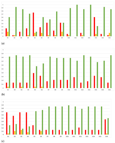
Figure 17.
Experiment 1: consistency per dataset. Rate of validity with the accuracy and time complexity. (a) Rate of vx per dataset in RF. In axis X, the dataset. In axis Y, the rate of RHOASo for each class of validity. (b) Rate of validity per dataset in GB. In axis X, the dataset. In axis Y, the rate of RHOASo for each class of validity. (c) Rate of validity per dataset in MLP. In axis X, the dataset. In axis Y, the rate of RHOASo for each class of validity.
In the case of MLP, there is a clear trend for the datasets in which RHOASo losses are , and . That is, datasets with a low number of instances (<10,000) but with a high number of features > 50. This failure in the large-dimension small-sized datasets can be due to the early-stop characteristic of the algorithm. Datasets with high dimensionality and low number of instances tend to increase the variance of the results, which contributes to create an irregular surface in , possibly trapping RHOASo in a local maximum. A possible solution could be to substitute the function that maps elements from the hyper-parameter space to the performance of the trained ML model on a validation dataset with an approximated probabilistic model of such function. This suggests that combining the underlying ideas of Bayesian hyper-parameter optimization algorithms with those presented in this paper could yield an early-stop algorithm that works efficiently in high dimensions.
In the case of RF, the gain of RHOASo is not enough for datasets , and . Unlike in the case of MLP, these datasets have no clear commonalities, so we can only hypothesize. We believe that the problem is the same as in the case of MLP: high variance in the results diminishes the effectiveness of RHOASo. However, in this case, this variance could be ascribed to the inherent randomness in the training of RF or in the cross validation sampling.
As we can see in Figure 18, the behavior of the rates of validity for each partition remains consistent when these are computed with the MCC and time complexity.
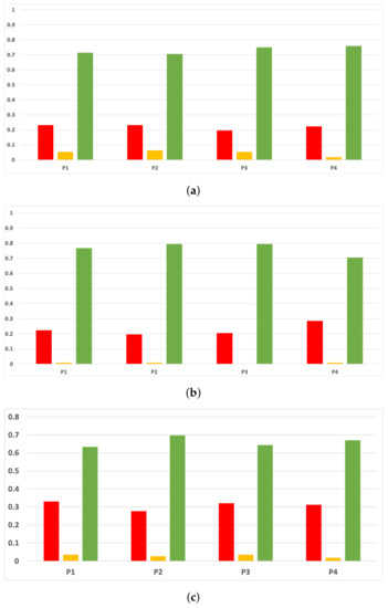
Figure 18.
Experiment 1: consistency per partition (MCC and time complexity). (a) Rate of validity per partition in RF. In axis X, the partition of the dataset. In axis Y, the rate of RHOASo for each class of validity. (b) Rate of validity per partition in GB. In axis X, the partition of the dataset. In axis Y, the rate of RHOASo for each class of validity. (c) Rate of validity per partition in MLP. In axis X, the partition of the dataset. In axis Y, the rate of RHOASo for each class of validity.
As we can see in Figure 19, the same conclusions as in the case of accuracy are obtained when we discriminate them by datasets. Nonetheless, the results concerning RF and MLP are not so far from being consistent (RF being closer than MLP), and a deeper analysis should be performed regarding this fact. We note that, in some cases, the green class is increased; this has not occurred for the red class in the unbalanced datasets.

Figure 19.
Consistency per dataset: rate of validity with the MCC and time complexity. (a) Rate of validity per dataset in RF. In axis X, the dataset. In axis Y, the rate of RHOASo for each class of validity. (b) Rate of validity per dataset in GB. In axis X, the dataset. In axis Y, the rate of RHOASo for each class of validity. (c) Rate of validity per dataset in MLP. In axis X, the dataset. In axis Y, the rate of RHOASo for each class of validity.
5.4.2. Experiment 2
The rates of validity for each partition computed with the accuracy and time complexity are included in Figure 20. In this experiment, RHOASo is more inconsistent since it loses the advantage of execution time that it had over the other HPOs. RHOASo has a consistent advantage for all partition sizes in GB, but for RF it only improves other algorithms for partitions 3 and 4 and is inferior in MLP in all partitions, although the results improve when the size of the partition increases. This trend is also present for RF and GB. The reasons for this trend are probably the same as those we discussed in Section 5.4.1: the variance in the results trapping RHOASo in the local maxima.
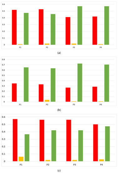
Figure 20.
Experiment 2: consistency per partition (accuracy and time complexity). (a) Rate of validity per partition in RF. In axis X, the partition of the dataset. In axis Y, the rate of RHOASo for each class of validity. (b) Rate of validity per partition in GB. In axis X, the partition of the dataset. In axis Y, the rate of RHOASo for each class of validity. (c) Rate of validity per partition in MLP. In axis X, the partition of the dataset. In axis Y, the rate of RHOASo for each class of validity.
As we can see in Figure 21, the validity per dataset is negatively affected. In RF, there is a general decrease, with only datasets 10, 12, 12 and 15 showing a clear advantage for RHOASo. For GB, RHOASo maintains better results than other algorithms for all datasets, except 5 and 6. However, the consistency is lower than in experiment 1. Finally, in MLP, the validity of RHOASo is the lowest among all models, being consistently outperformed in five datasets: 1, 2, 3, 4 and 13.
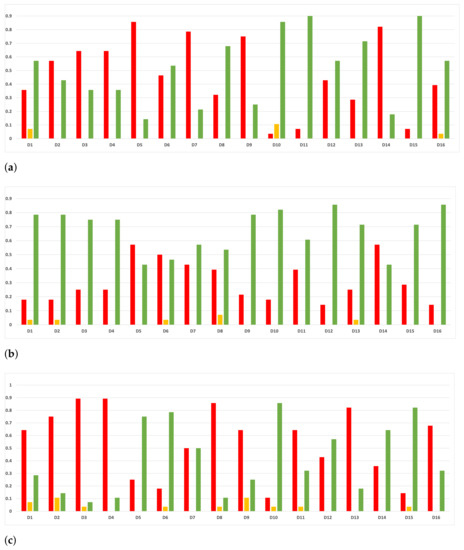
Figure 21.
Experiment 2: consistency per dataset. Rate of validity with the accuracy and time complexity. (a) Rate of validity per dataset in RF. In axis X, the dataset. In axis Y, the rate of RHOASo for each class of validity. (b) Rate of validity per dataset in GB. In axis X, the dataset. In axis Y, the rate of RHOASo for each class of validity. (c) Rate of validity per dataset in MLP. In axis X, the dataset. In axis Y, the rate of RHOASo for each class of validity.
The datasets with the worst results for each model have no clear commonalities, so it is possible that the neutralization of the execution time advantage of RHOASo is a significant factor in the deterioration of the results.
In Figure 22, we show the results of the above analysis with the MCC and the time time complexity. The results are very similar to those achieved with accuracy. The main difference is that the validity for RF is improved for partitions 1 and 2, increasing the consistency of the results.
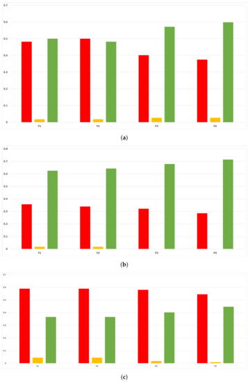
Figure 22.
Experiment 2: consistency per partition (MCC and time complexity). (a) Rate of validity per partition in RF. In axis X, the partition of the dataset. In axis Y, the rate of RHOASo for each class of validity. (b) Rate of validity per partition in GB. In axis X, the partition of the dataset. In axis Y, the rate of RHOASo for each class of validity. (c) Rate of validity per partition in MLP. In axis X, the partition of the dataset. In axis Y, the rate of RHOASo for each class of validity.
In Figure 23, we show the rate of validity per dataset, using the MCC as the reference metric. As happened in Experiment 1, the trends are mostly the same as those present when evaluating the accuracy.
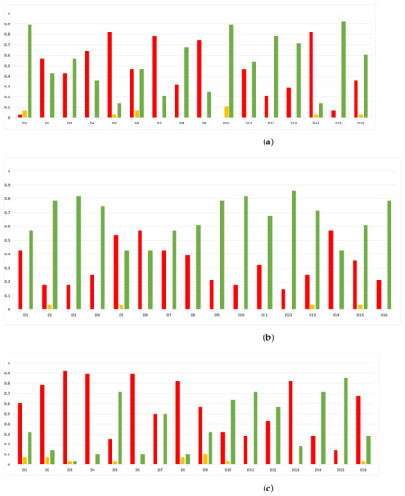
Figure 23.
Experiment 2: consistency per dataset. Rate of validity with the MCC and time complexity. (a) Rate of validity per dataset in RF. In axis X, the dataset. In axis Y, the rate of RHOASo for each class of validity. (b) Rate of validity per dataset in GB. In axis X, the dataset. In axis Y, the rate of RHOASo for each class of validity. (c) Rate of validity per dataset in MLP. In axis X, the dataset. In axis Y, the rate of RHOASo for each class of validity.
6. Conclusions
ML provides several powerful tools for data processing that find applications in different fields. Most of the existent models have several hyper-parameters that need to be tuned and have a noticeable impact on their performance. Therefore, HPO algorithms are essential to achieve the highest possible accuracy with minimal human intervention.
In this work, a new HPO algorithm is described as a generalization of the discrete analog of a basic iterative algorithm to obtain the solutions to certain conditional optimization problems for the logistic function. It is shown that its performance is weakly disturbed by changing the size of the data subset with which it is run. The algorithm shows positive statistically meaningful differences in efficiency, regarding the other HPO algorithms considered in this study. The algorithm can finish the tuning process by itself and only requires an upper bound on the number of iterations to perform. Furthermore, it is shown that, on average, it needs around of the iterations needed by the other hyper-parameter optimization algorithms to achieve competitive results.
The results show that the algorithm achieves high accuracy, with similar results for all classifiers on each dataset. In addition, RHOASo can effectively use a small partition size to accelerate the HPO process without sacrificing the final accuracy of the model. Lastly, the automatic early stop ends the tuning process before reaching the fixed number of iterations (), further increasing its efficiency.
Future work can be aimed at several lines:
- Test the RHOASO’s performance with more machine learning algorithms, such as decision trees or k-nearest neighbors.
- Include more HPO algorithms in the comparison of the effectivity of RHOASo.
- Optimize RHOASo so it can be effective on search spaces of greater dimensions and can better deal with an extremely indented surface of , possibly using a surrogate of the target function, such as in Bayesian optimization.
- Factor the possible inclusion and effect of parallelization.
- Assess RHOASo on data streams.
Author Contributions
Conceptualization: Á.L.M.C.; methodology: Á.L.M.C. and N.D.-G.; software: Á.L.M.C. and D.E.G.; validation: all authors have contributed equally; formal analysis: N.D.-G. and D.E.G.; investigation: Á.L.M.C. and N.D.-G.; data curation: D.E.G.; writing—original draft preparation, review and editing: all authors have contributed equally; project administration and funding acquisition: N.D.-G. All authors have read and agreed to the published version of the manuscript.
Funding
This work was partially supported by the Spanish National Cybersecurity Institute (INCIBE) under contract Art.83, key: X54.
Data Availability Statement
The datasets supporting this work are from previously reported studies and datasets, which are cited. The processed data are available from the corresponding author upon request.
Acknowledgments
The authors would like to thank the Spanish National Cybersecurity Institute (INCIBE), who partially supported this work. Additionally, in this research, the resources of the Center of Supercomputation of Castilla y León (SCAYLE) were used.
Conflicts of Interest
The authors declare no conflict of interest. The funders had no role in the design of the study; in the collection, analyses, or interpretation of data; in the writing of the manuscript, or in the decision to publish the results.
Abbreviations
The following abbreviations are used in this manuscript:
| CMA-ES | Covariance Matrix Adaptation Evolutionary |
| GB | Gradient Boosting |
| HPO | Hyper-Parameters Optimization |
| ML | Machine Learning |
| MLP | Multi-Layer Perceptron |
| NM | Nelder-Mead |
| PS | Particle Swarm |
| RBFOpt | Radial Basis Function Optimization |
| RF | Random Forest |
| RS | Random Search |
| SMAC | Sequential Model Automatic Configuration |
| SMBO | Sequential Model-Based Optimization |
| TPE | Tree Parzen Estimators |
Appendix A. Additional Results
In this appendix, we show the results concerning Experiment 1 in the case that the ML algorithms are DT and KNN. Due to the great difference in the performance of RHOASo with respect to the rest of the HPO algorithms when they are run with these ML algorithms, we have excluded the analyses from the body of the article. However, we believe that the obtained results may be of interest.
We give a brief description of DT and KNN below.
- DT is a tree-like model, where the internal nodes and their edges encode possibilities and the ending nodes (leafs) encode decisions. Te maximum length of the paths joining the root node and a leaf is called the depth of the tree. There are a number of DT training algorithms, among which we can point out ID3, ID4, ID5 and CART. In this study, we have chosen CART.
- KNN is a non-parametric classification model the may be also used in regression problems. The training examples are simply vectors in the feature space, carrying their class label. The training phase does not consist of constructing an internal mathematical model but simply allocating training data instances in the feature space. The classification phase is done by looking at the majority label of the k-nearest neighbors of each point. This implies the choice of a metric on the feature space, which by default is usually taken as the Minkowski distance.
In Table A1, we include the hyper-parameters that we have tuned. We have chosen them because of their influence on the corresponding ML algorithms (see [3], Appendixes A1, A4). Concerning the hyper-parameters of DT to be tuned, we have chosen the minimum number of samples required to split an internal node (min_smaples_split) and the minimum number of samples required to be at a leaf node (min_samples_leaf). Regarding the hyper-parameters of KNN, we have considered the number of neighbors to use for queries and p, the Minkowski’s distance type.
The search space for all hyper-parameters is in the interval [1, 50]. All hyper-parameters not being tuned are set to their default values in scikit-learn implementation ([34]). We have used 10-fold cross-validation to assess the performance of all ML models combined with the HPO algorithms.
Table A1.
ML algorithms together with hyper-parameters we have considered.
Table A1.
ML algorithms together with hyper-parameters we have considered.
| Name | Hyper-Parameter 1 | Hyper-Parameter 2 |
|---|---|---|
| DT | min_smaples_split | min_samples_leaf |
| KNN | n_neighbors | p |
Appendix A.1. Performance of RHOASo
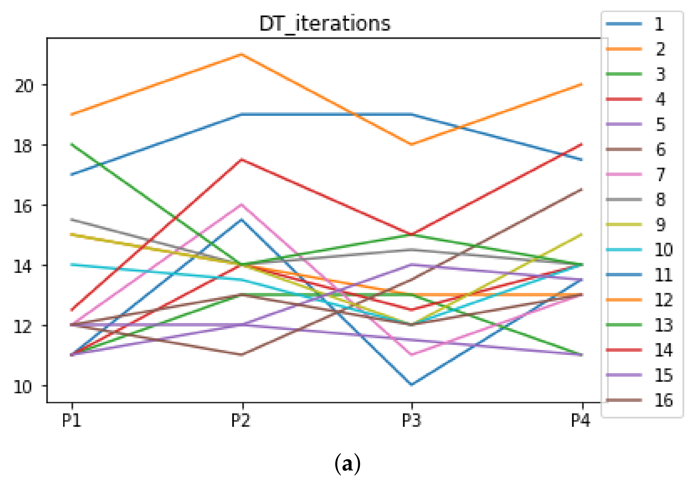
We can see in Figure A1, Figure A2, Figure A3, Figure A4, Figure A5 and Figure A6 that we have plotted the median of the accuracy, MCC, total time, sensitivity, specificity, and the number of iterations when RHOASo is applied together with DT and KNN. The median of accuracy for DT over all datasets is and for KNN, it is . We can observe that the achieved accuracy by RHOASo presents great stability in terms of partitions of the dataset, except for partition P4 and some datasets. The median of MCC for DT is , and for KNN it is . Again, RHOASo presents a similar behavior to the accuracy. It can be due to does not contribute to improve the fit of the models, see [1]. Regarding the time complexity, the median value for DT is s, and for KNN it is seconds. It can be shown that the total time registered for in KNN is higher in than in . This can be caused because the stabilizer of RHOASo achieves an optimum value before in the total dataset compared to . The median of sensitivity is for DT, and for KNN. In contrast, specificity has a median of for DT, and for KNN. In addition, these plots inherit the same trends as the graphics of the accuracy and MCC. The median of the number of iterations for DT is 14, and for KNN it is 19. It is worth pointing out the number of iterations for is larger than for when we work with KNN in . This is probably caused by the same reason as in the plot of the total time.
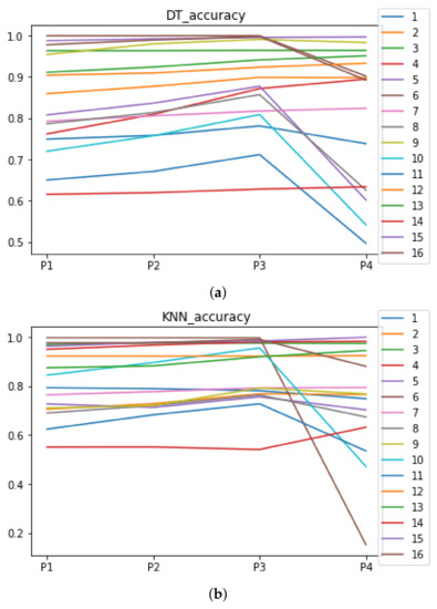
Figure A1.
Behavior of RHOASo: accuracy. Each line represents a dataset. (a) Accuracy for DT. (b) Accuracy for KNN.
Figure A1.
Behavior of RHOASo: accuracy. Each line represents a dataset. (a) Accuracy for DT. (b) Accuracy for KNN.
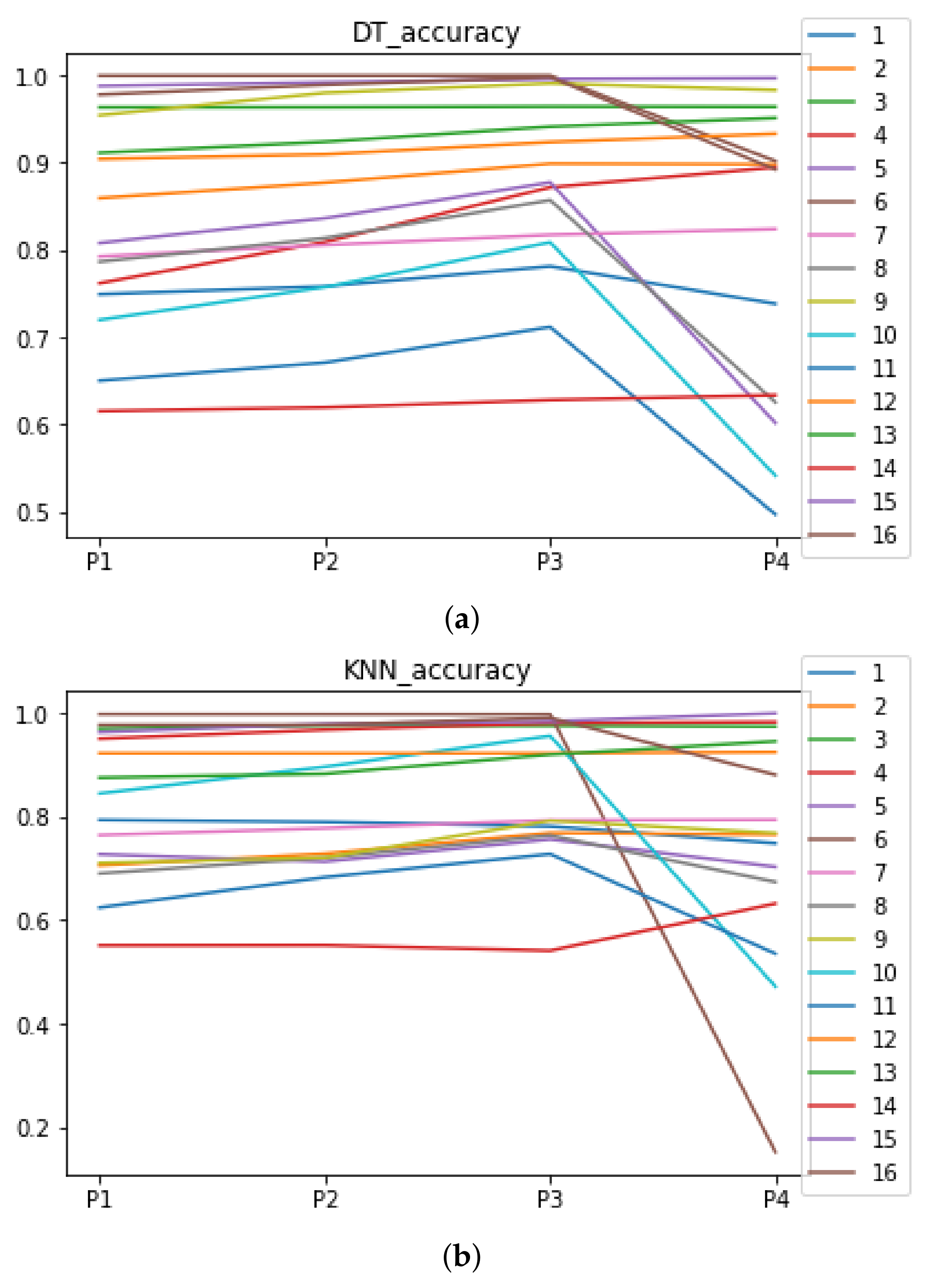
Figure A2.
Behavior of RHOASo: MCC. Each line represents a dataset. (a) MCC for DT. (b) MCC for KNN.
Figure A2.
Behavior of RHOASo: MCC. Each line represents a dataset. (a) MCC for DT. (b) MCC for KNN.
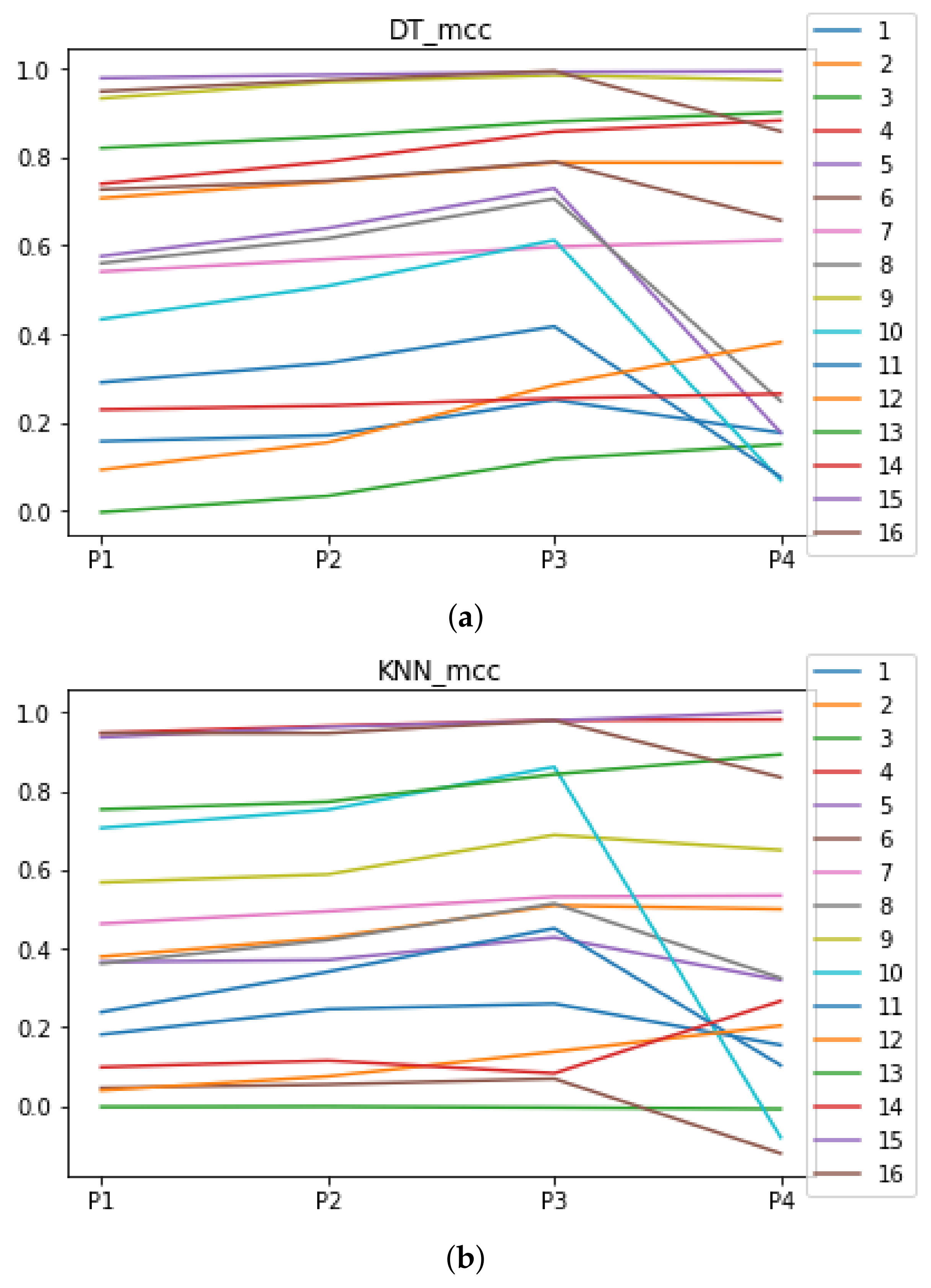
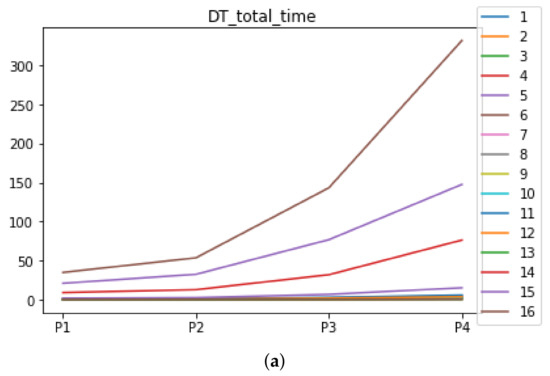
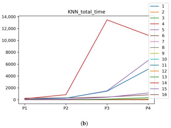
Figure A3.
Behavior of RHOASo: time complexity. Each line represents a dataset. (a) Time complexity for DT. (b) Time complexity for KNN.
Figure A3.
Behavior of RHOASo: time complexity. Each line represents a dataset. (a) Time complexity for DT. (b) Time complexity for KNN.

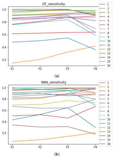
Figure A4.
Behavior RHOASo: sensitivity. The datasets are represented with a bar chart for each partition. (a) Sensitivity for DT. (b) Sensitivity for KNN.
Figure A4.
Behavior RHOASo: sensitivity. The datasets are represented with a bar chart for each partition. (a) Sensitivity for DT. (b) Sensitivity for KNN.
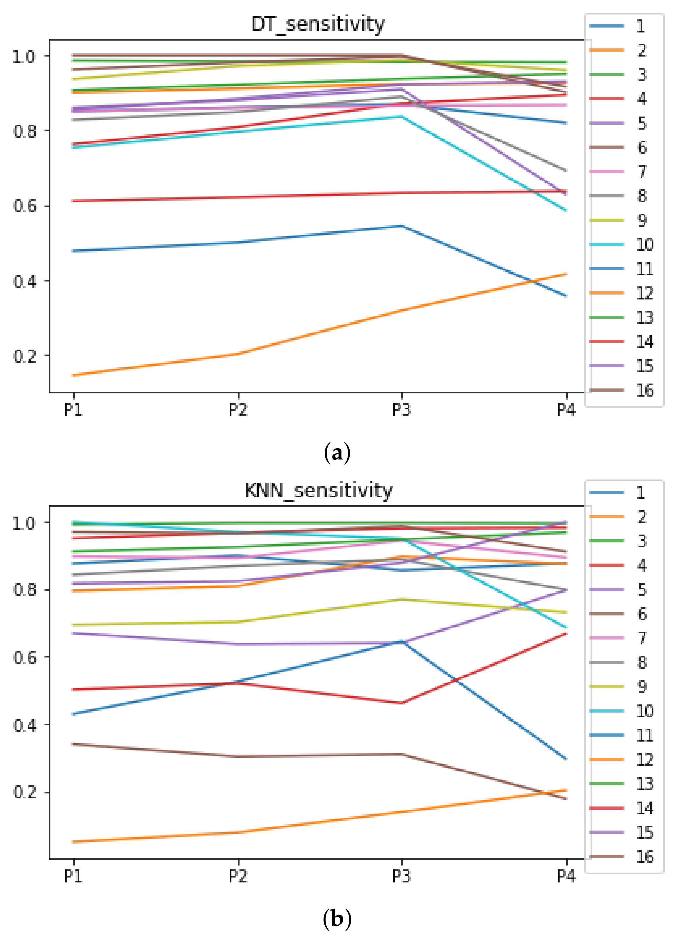

Figure A5.
Behavior RHOASo: specificity. The datasets are represented with a bar chart for each partition. (a) Specificity for DT. (b) Specificity for KNN.
Figure A5.
Behavior RHOASo: specificity. The datasets are represented with a bar chart for each partition. (a) Specificity for DT. (b) Specificity for KNN.
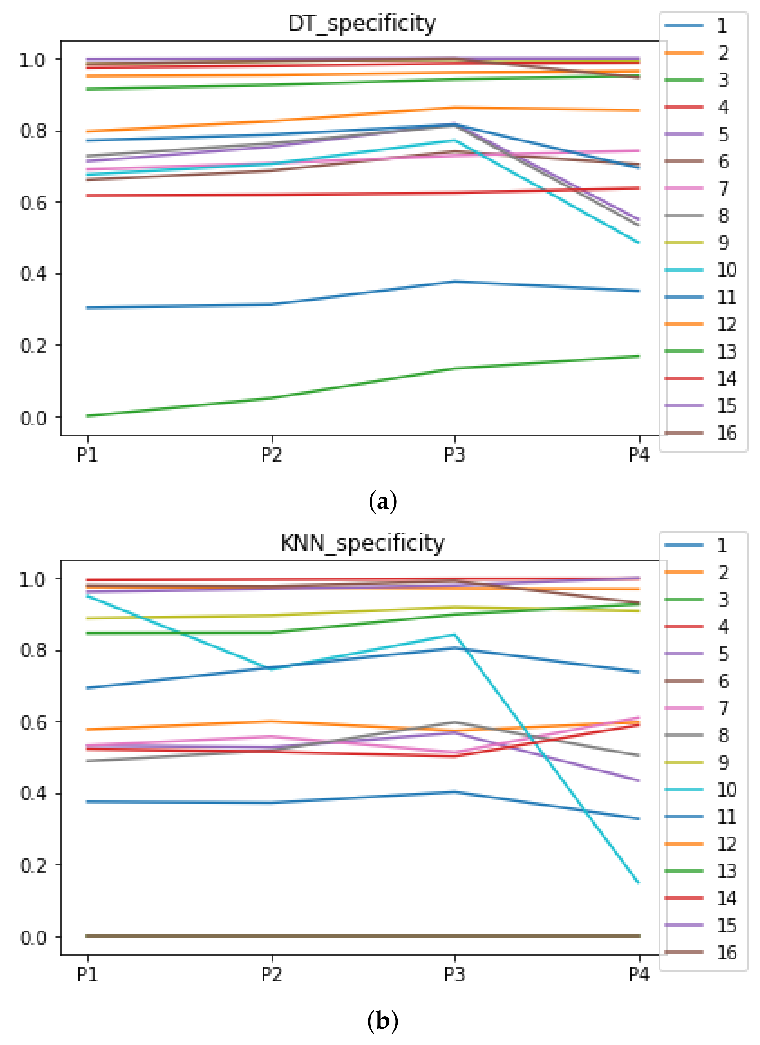
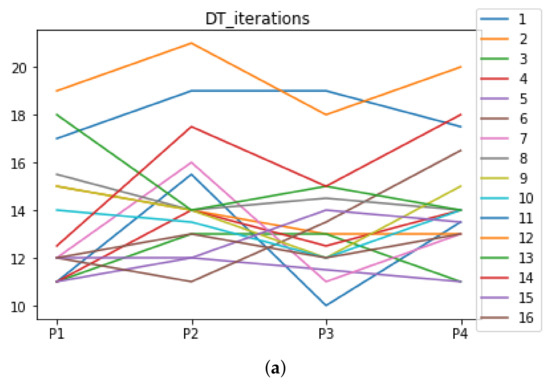
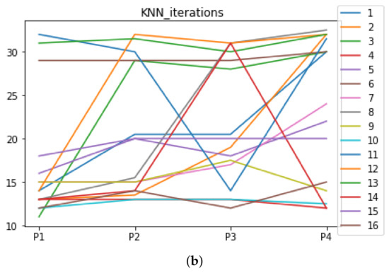
Figure A6.
Number of iterations per partition. Each line represents a dataset (medians). (a) Number of iterations DT. (b) Number of iterations KNN.
Figure A6.
Number of iterations per partition. Each line represents a dataset (medians). (a) Number of iterations DT. (b) Number of iterations KNN.
Appendix A.2. Are There Statistically Meaningful Differences between the Performance of RHOASo and the Other HPO Algorithms under DT and KNN?
In Figure A7 and Figure A8, the performances (accuracies and time complexities) that are achieved by the HPO algorithms over each dataset are shown.
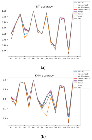
Figure A7.
Accuracy complexity. (a) Accuracy in DT. (b) Accuracy in KNN.
Figure A7.
Accuracy complexity. (a) Accuracy in DT. (b) Accuracy in KNN.

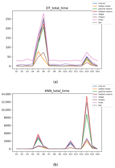
Figure A8.
Time complexity. (a) Time complexity in DT. (b) Time complexity in KNN.
Figure A8.
Time complexity. (a) Time complexity in DT. (b) Time complexity in KNN.
The results of validity of RHOASo faced on the rest of HPO algorithms are included in Table A2, which show that, on average, the class corresponding to positive statistically significative differences is higher than . Note that these computations are carried out with the accuracies and time complexities by the analyses that are explained in Section 4.4.
Table A2.
Rate of validity of RHOASo vs. HPO across all (% with accuracy and time complexity).
Table A2.
Rate of validity of RHOASo vs. HPO across all (% with accuracy and time complexity).
| Validity | DT | KNN | Average |
|---|---|---|---|
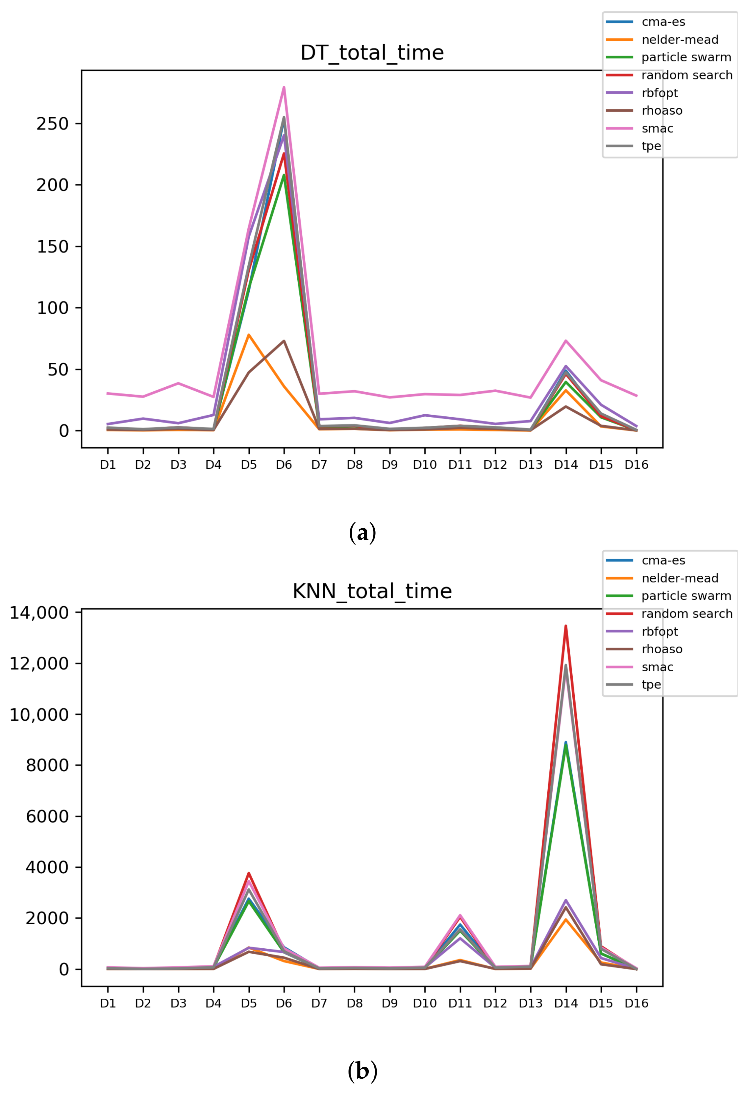
Since we have dealt with unbalanced datasets, we have repeated the analyses, changing the metric of accuracy by MCC so as to avoid over-optimistic scores. In Figure A9, the MCCs that are achieved by the HPO algorithms over each dataset are shown.

Figure A9.
MCC of all HPO algorithms. (a) MCC in DT. (b) MCC in KNN.
Figure A9.
MCC of all HPO algorithms. (a) MCC in DT. (b) MCC in KNN.
The rates of validity that are obtained by RHOASo, compared to the rest of HPO of algorithms with the MCCs and time complexities, are included in Table A3.
Table A3.
Rate of validity of RHOASo vs. HPO across all (% with MCC and time complexity).
Table A3.
Rate of validity of RHOASo vs. HPO across all (% with MCC and time complexity).
| Validity | DT | KNN | Average |
|---|---|---|---|
We can observe that the rate of gain of RHOASo overcomes the 89% of the cases.
Appendix A.3. Are the above Results Consistent?
In this section, we analyze whether RHOASo achieves a significant performance improvement consistently across datasets and partitions.
The rates of validity for each partition computed with the accuracy and time complexity are included in Figure A10. As can be seen, RHOASo presents a much higher performance than any other HPO algorithm taken into account in this work, and this behavior is independent of the partition.
Figure A10.
Experiment 1: consistency per partition (accuracy and time complexity). (a) Rate of validity per partition in DT. (b) Rate of validity per partition in KNN.
Figure A10.
Experiment 1: consistency per partition (accuracy and time complexity). (a) Rate of validity per partition in DT. (b) Rate of validity per partition in KNN.
As we can see in Figure A11, the above conclusion is the same when we discriminate rates of validity by datasets.
As we can see in Figure A12, the behavior of the rates of validity for each partition remains consistent when these are computed with the MCC and time complexity. As we can seen in Figure A13, the same conclusion as in the case of accuracy is obtained when we discriminate them by datasets.
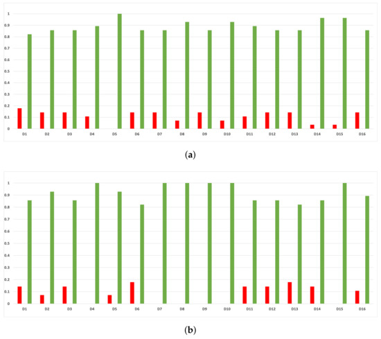
Figure A11.
Experiment 1: consistency per dataset. Rate of validity with the accuracy and time complexity. (a) Rate of validity per dataset in DT. (b) Rate of validity per dataset in KNN.
Figure A11.
Experiment 1: consistency per dataset. Rate of validity with the accuracy and time complexity. (a) Rate of validity per dataset in DT. (b) Rate of validity per dataset in KNN.
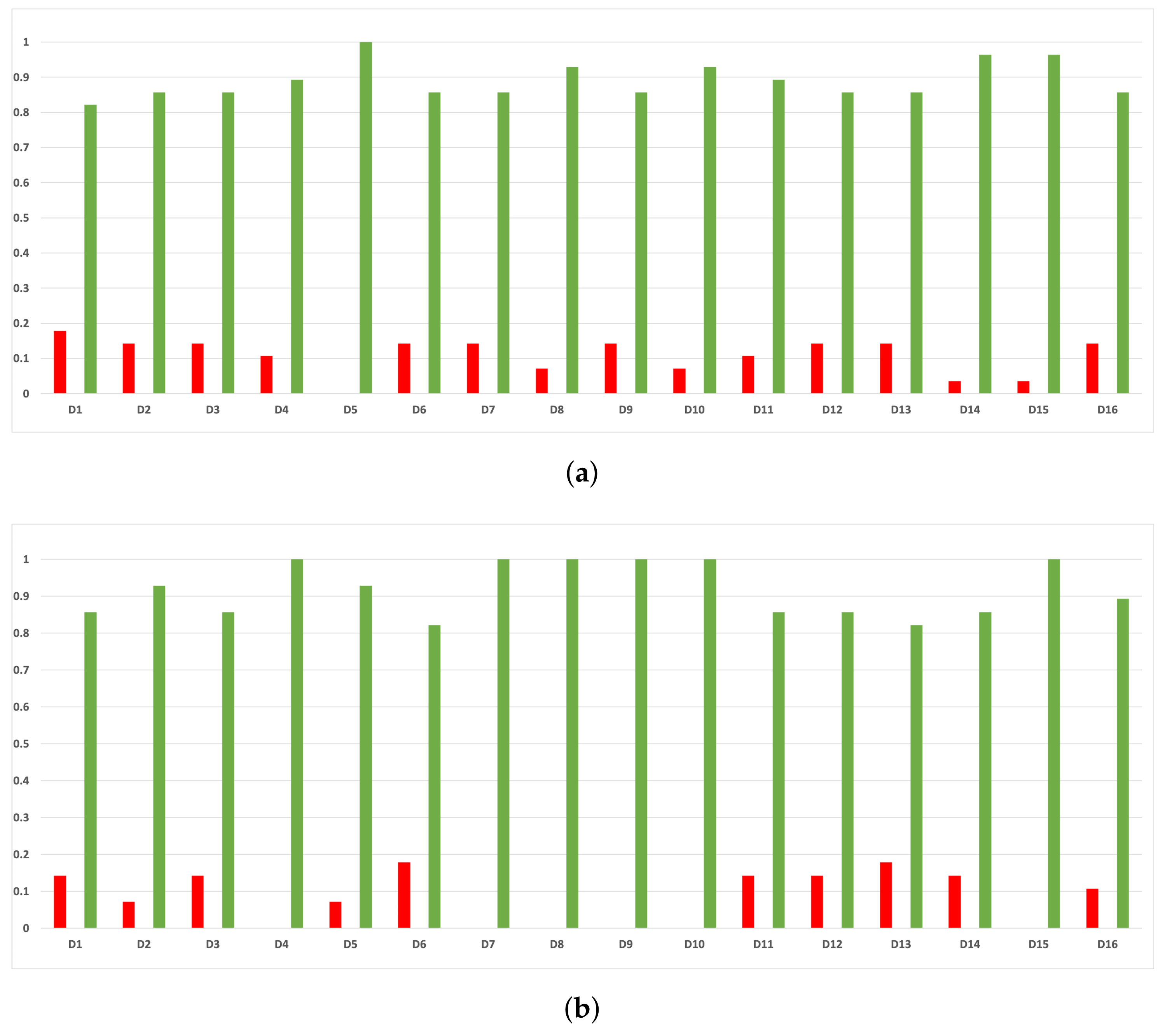
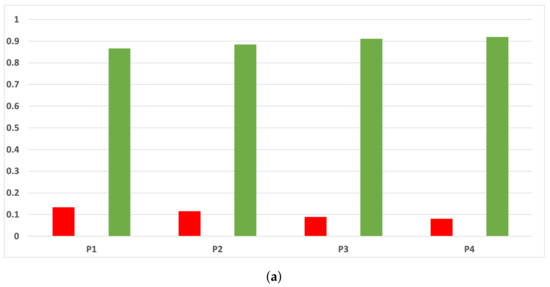
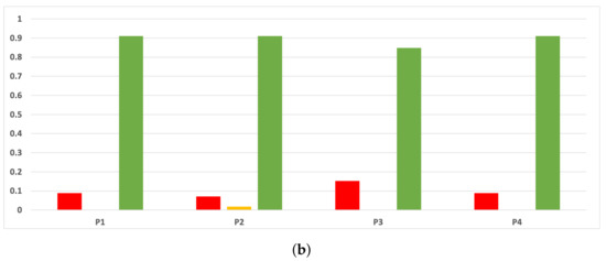
Figure A12.
Experiment 1: consistency per partition (MCC and time complexity). (a) Rate of validity per partition in DT. (b) Rate of validity per partition in KNN.
Figure A12.
Experiment 1: consistency per partition (MCC and time complexity). (a) Rate of validity per partition in DT. (b) Rate of validity per partition in KNN.
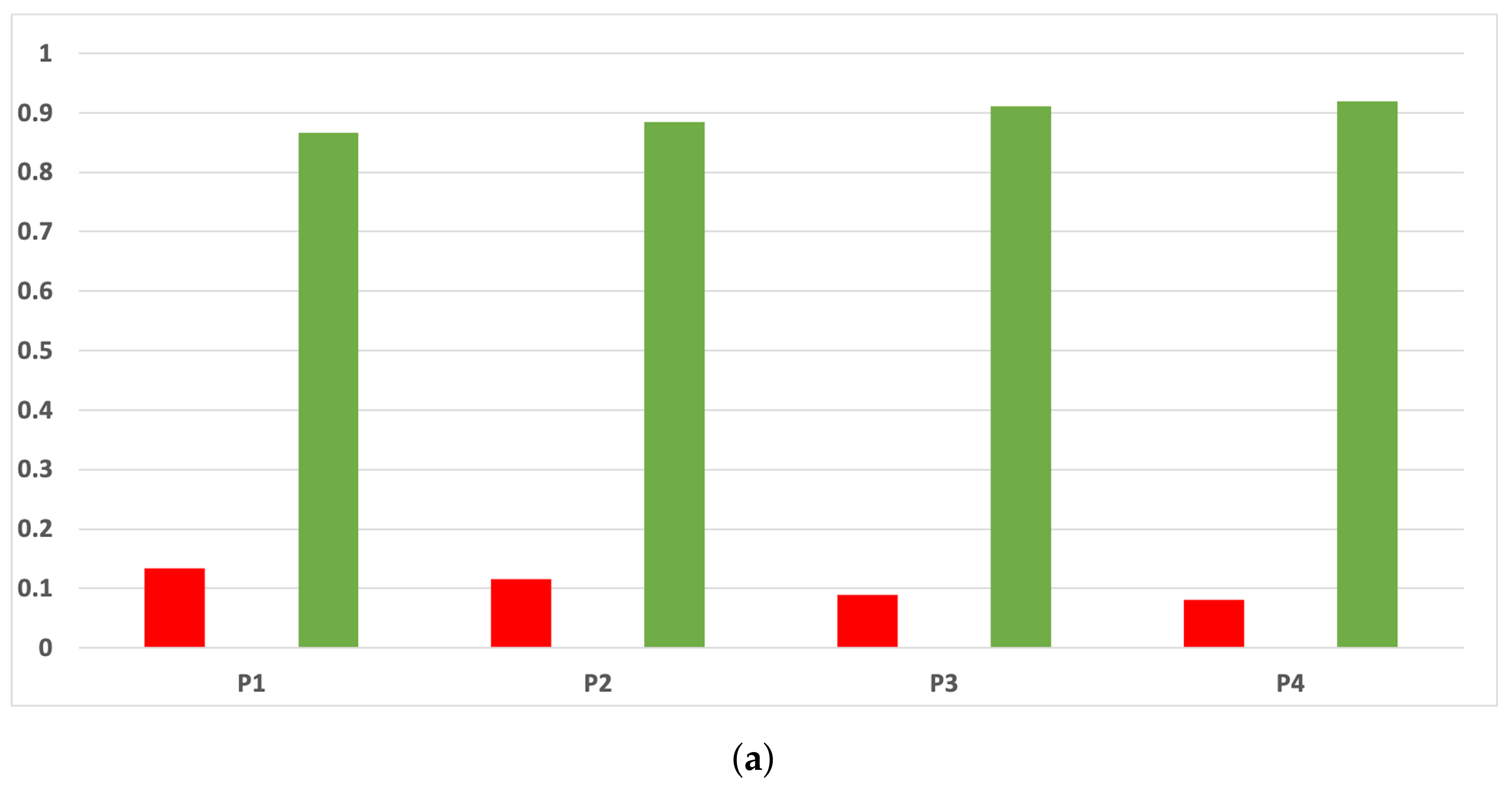
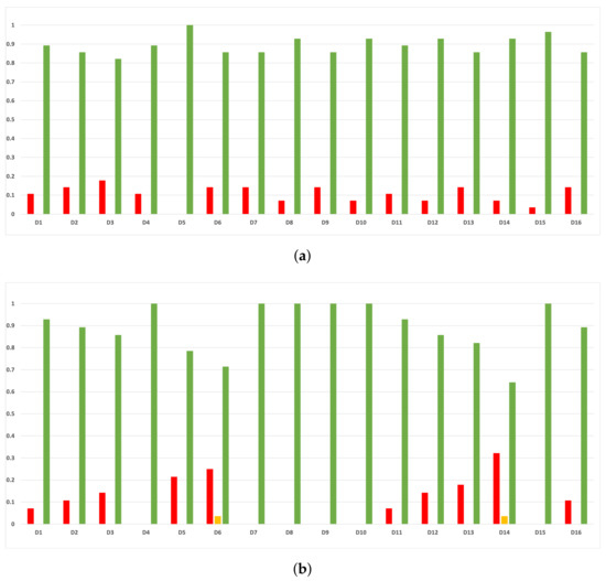
Figure A13.
Consistency per dataset: rate of validity with the MCC and time complexity. (a) Rate of validity per dataset in DT. (b) Rate of validity per dataset in KNN.
Figure A13.
Consistency per dataset: rate of validity with the MCC and time complexity. (a) Rate of validity per dataset in DT. (b) Rate of validity per dataset in KNN.

References
- DeCastro-García, N.; Muñoz Castañeda, A.L.; Escudero García, D.; Carriegos, M. Effect of the Sampling of a Dataset in the Hyperparameter Optimization Phase over the Efficiency of a Machine Learning Algorithm. Complexity 2019, 2019, 16. [Google Scholar] [CrossRef]
- Jamieson, K.; Talwalkar, A. Non-stochastic best arm identification and hyperparameter optimization. In Proceedings of the 19th International Conference on Artificial Intelligence and Statistics, AISTATS 2016, Cadiz, Spain, 9–11 May 2016; pp. 240–248. [Google Scholar]
- Bischl, B.; Binder, M.; Lang, M.; Pielok, T.; Richter, J.; Coors, S.; Thomas, J.; Ullmann, T.; Becker, M.; Boulesteix, A.L.; et al. Hyperparameter Optimization: Foundations, Algorithms, Best Practices and Open Challenges. arXiv 2021, arXiv:stat.ML/2107.05847. [Google Scholar]
- Bengio, Y. Gradient-Based Optimization of Hyperparameters. Neural Comput. 2000, 12, 1889–1900. [Google Scholar] [CrossRef]
- Maclaurin, D.; Duvenaud, D.; Adams, R. Gradient-based hyperparameter optimization through reversible learning. In Proceedings of the 32nd International Conference on Machine Learning (ICML’15). IMLS, Lille, France, 6–11 July 2015; Volume 37, pp. 2113–2122. [Google Scholar]
- Franceschi, L.; Donini, M.; Frasconi, P.; Pontil, M. Forward and Reverse Gradient-Based Hyperparameter Optimization. In Proceedings of the 34th International Conference on Machine Learning, Sydney, NSW, Australia, 6–11 August 2017; Precup, D., Teh, Y.W., Eds.; PMLR: International Convention Centre: Sydney, Australia, 2017; Volume 70, pp. 1165–1173. [Google Scholar]
- Mockus, J. On Bayesian Methods for Seeking the Extremum. In Proceedings of the IFIP Technical Conference; Springer: London, UK, 1974; pp. 400–404. [Google Scholar]
- Snoek, J.; Larochelle, H.; Adams, R.P. Practical Bayesian Optimization of Machine Learning Algorithms. In Proceedings of the 25th International Conference on Neural Information Processing Systems (NIPS’12), Lake Tahoe, NV, USA, 3–6 December 2012; Curran Associates Inc.: New York, NY, USA, 2012; Volume 2, pp. 2951–2959. [Google Scholar]
- Hutter, F.; Hoos, H.H.; Leyton-Brown, K. Sequential Model-based Optimization for General Algorithm Configuration. In Proceedings of the 5th International Conference on Learning and Intelligent Optimization, Rome, Italy, 17–21 January 2011; Springer: Berlin, Heidelberg, 2011. LION’05. pp. 507–523. [Google Scholar] [CrossRef] [Green Version]
- Bergstra, J.; Bardenet, R.; Bengio, Y.; Kégl, B. Algorithms for Hyper-parameter Optimization. In Proceedings of the 24th International Conference on Neural Information Processing Systems, Granada, Spain, 12–15 December 2011; Curran Associates Inc.: New York, USA, 2011. NIPS’11. pp. 2546–2554. [Google Scholar]
- IIlievski, l.; Akhtar, T.; Feng, J.; Shoemaker, C.A. Efficient hyperparameter optimization for deep learning algorithms using deterministic RBF surrogates. In Proceedings of the Thirty-First AAAI Conference on Artificial Intelligence, San Francisco, CA, USA, 4–9 February 2017; pp. 822–829. [Google Scholar]
- Hernández-Lobato, J.M.; Hoffman, M.W.; Ghahramani, Z. Predictive Entropy Search for Efficient Global Optimization of Black-box Functions. In Proceedings of the 27th International Conference on Neural Information Processing Systems (NIPS’14), Montreal, QC, Canada, 8–13 December 2017; MIT Press: Cambridge, MA, USA, 2014; Volume 1, pp. 918–926. [Google Scholar]
- Bardenet, R.; Brendel, M.; Kégl, B.; Sebag, M. Collaborative Hyperparameter Tuning. In Proceedings of the 30th International Conference on Machine Learning (ICML’13), Atlanta, GA, USA, 16–21 June 2013; Volume 28, pp. 858–866. [Google Scholar]
- Swersky, K.; Snoek, J.; Adams, R.P. Multi-task Bayesian Optimization. In Proceedings of the 26th International Conference on Neural Information Processing Systems (NIPS’13), Lake Tahoe, NV, USA, 5–10 December 2013; Curran Associates Inc.: New York, USA, 2013; Volume 2, pp. 2004–2012. [Google Scholar]
- Bergstra, J.; Bengio, Y. Random search for hyper-parameter optimization. J. Mach. Learn. Res. 2012, 13, 281–305. [Google Scholar]
- Nuñez, L.; Regis, R.G.; Varela, K. Accelerated Random Search for constrained global optimization assisted by Radial Basis Function surrogates. J. Comput. Appl. Math. 2018, 340, 276–295. [Google Scholar] [CrossRef]
- Hansen, N.; Ostermeier, A. Completely Derandomized Self-Adaption in Evolution Strategies. Evol. Comput. 2001, 9, 159–195. [Google Scholar] [CrossRef]
- Nelder, J.; Mead, R. A simplex method for function minimization. Comput. J. 1965, 7, 308–313. [Google Scholar] [CrossRef]
- Ozaki, Y.; Yano, M.; Onishi, M. Effective hyperparameter optimization using Nelder-Mead method in deep learning. Ipsj Trans. Comput. Vis. Appl. 2017, 9, 20. [Google Scholar] [CrossRef] [Green Version]
- Clerc, M.; Kennedy, J. The particle swarm-explosion, stability, and convergence in a multidimensional complex space. IEEE Trans. Evol. Comput. 2002, 6, 58–73. [Google Scholar] [CrossRef] [Green Version]
- Fortin, F.; De Rainville, F.; Gardner, M. DEAP: Evolutionary Algorithms Made Easy. J. Mach. Learn. Res. 2012, 13, 2171–2175. [Google Scholar]
- Li, L.; Jamieson, K.; DeSalvo, G.; Rostamizadeh, A.; Talwalkar, A. Hyperband: A novel bandit-based approach to hyperparameter optimization. J. Mach. Learn. Res. 2018, 18, 1–52. [Google Scholar]
- Li, L.; Jamieson, K.; Rostamizadeh, A.; Gonina, E.; Ben-Tzur, J.; Hardt, M.; Recht, B.; Tal-Walkar, A. A System for Massively Parallel Hyperparameter Tuning. In Proceedings of the Machine Learning and Systems 2020, Austin, TX, USA, 2–4 March 2020; pp. 230–246. [Google Scholar]
- Falkner, S.; Klein, A.; Hutter, F. BOHB: Robust and Efficient Hyperparameter Optimization at Scale. In Proceedings of the 35th International Conference on Machine Learning. PMLR, Stockholm, Sweden, 10–15 July 2018; Volume 80, pp. 1437–1446. [Google Scholar]
- Bergstra, J.; Yamins, D.; Cox, D. Hyperopt: A python library for optimizing the hyperparameters of machine learning algorithms. In Proceedings of the 12th Python in Science Conference (SCIPY 2013), Austin, TX, USA, 24–28 June 2013; pp. 13–20. [Google Scholar] [CrossRef]
- Claesen, M.; Simm, J.; Popovic, D.; Moreau, Y.; De Moor, B. Easy Hyperparameter Search Using Optunity. arXiv 2014, arXiv:1412.1114. [Google Scholar]
- Lindauer, M.; Eggensperger, K.; Feurer, M.; Falkner, S.; Biedenkapp, A.; Hutter, F. SMAC v3: Algorithm Configuration in Python. 2017. Available online: https://github.com/automl/SMAC3 (accessed on 25 July 2021).
- Costa, A.; Nannicini, G. RBFOpt: An open-source library for black-box optimization with costly function evaluations. Math. Program. Comput. 2018, 10, 597–629. [Google Scholar] [CrossRef]
- DeCastro-García, N.; Castañeda, Á.L.M.; Fernández-Rodríguez, M. RADSSo: An Automated Tool for the multi-CASH Machine Learning Problem. In Hybrid Artificial Intelligent Systems; de la Cal, E.A., Villar Flecha, J.R., Quintián, H., Corchado, E., Eds.; Springer International Publishing: Cham, Switzerland, 2020; pp. 183–194. [Google Scholar]
- DeCastro-García, N.; Castañeda, Á.L.M.; Fernández-Rodríguez, M. Machine learning for automatic assignment of the severity of cybersecurity events. Comput. Math. Methods 2020, 2, e1072. [Google Scholar] [CrossRef] [Green Version]
- Breiman, L. Random Forests. Mach. Learn. 2001, 45, 5–32. [Google Scholar] [CrossRef] [Green Version]
- Friedman, J. Greedy function approximation: A gradient boosting machine. Ann. Statist. 2001, 29, 1189–1232. [Google Scholar] [CrossRef]
- Friedman, J. Stochastic gradient boosting. Comput. Stat. Data Anal. 2002, 38, 367–378. [Google Scholar] [CrossRef]
- Pedregosa, F.; Varoquaux, G.; Gramfort, A.; Michel, V.; Thirion, B.; Grisel, O.; Blondel, M.; Prettenhofer, P.; Weiss, R.; Dubourg, V.; et al. Scikit-learn: Machine Learning in Python. J. Mach. Learn. Res. 2011, 12, 2825–2830. [Google Scholar]
- Guo, X.; Yang, J.; Wu, C.; Wang, C.; Liang, Y. A novel LS-SVMs hyper-parameter selection based on particle swarm optimization. Neurocomputing 2008, 71, 3211–3215. [Google Scholar] [CrossRef]
- Diaz, G.I.; Fokoue-Nkoutche, A.; Nannicini, G.; Samulowitz, H. An effective algorithm for hyperparameter optimization of neural networks. Ibm J. Res. Dev. 2017, 61, 9:1–9:11. [Google Scholar] [CrossRef] [Green Version]
- Bridge, J.P.; Holden, S.B.; Paulson, L.C. Machine Learning for First-Order Theorem Proving. J. Autom. Reason. 2014, 53, 141–172. [Google Scholar] [CrossRef]
- Hopkins, E.M.; Reeber, G.F. Datataset Spambase. UCI Machine Learning Repository. 1998. Available online: https://archive.ics.uci.edu/ml/datasets/spambase (accessed on 27 August 2019).
- Zieba, M.; Tomczak, S.; Tomczak, J. Ensemble boosted trees with synthetic features generation in application to bankruptcy prediction. Expert Syst. Appl. 2016, 58, 93–101. [Google Scholar] [CrossRef]
- Alpaydin, E.; Kaynak, C. Optical Recognition of Handwritten Digits Dataset. UCI Machine Learning Repository. 1995. Available online: https://archive.ics.uci.edu/ml/datasets/Optical+Recognition+of+Handwritten+Digits (accessed on 27 August 2019).
- De Almeida Freitas, F.; Peres, S.M.; De Moraes Lima, C.A.; Barbosa, F.V. Grammatical Facial Expressions recognition with Machine Learning. In Proceedings of the 27th International Florida Artificial Intelligence Research Society Conference, FLAIRS 2014, Pensacola Beach, FL, USA, 21–23 May 2014; pp. 180–185. [Google Scholar]
- Pozzolo, A.D.; Caelen, O.; Johnson, R.A.; Bontempi, G. Calibrating Probability with Undersampling for Unbalanced Classification. In Proceedings of the 2015 IEEE Symposium Series on Computational Intelligence, Cape Town, South Africa, 8–10 December 2015; pp. 159–166. [Google Scholar] [CrossRef]
- Bock, R.; Chilingarian, A.; Gaug, M. Methods for multidimensional event classification: A case study using images from a Cherenkov gamma-ray telescope. Nucl. Instr. Methods Phys. Res. Sect. Accel. Spectrom. Detect. Assoc. Equip. 2004, 516, 511–528. [Google Scholar] [CrossRef]
- Harries, M. SPLICE-2 Comparative Evaluation: Electricity Pricing. In Technical Report; The University of South Wales: Cardiff, UK, 1999. [Google Scholar]
- Gama, J.; Medas, P.; Castillo, G.; Rodrigues, P. Learning with Drift Detection. In Advances in Artificial Intelligence—SBIA 2004; Bazzan, A.L.C., Labidi, S., Eds.; Springer: Berlin/Heidelberg, Germany, 2004; pp. 286–295. [Google Scholar]
- Freire, A.L.; Barreto, G.A.; Veloso, M.; Varela, A.T. Short-term memory mechanisms in neural network learning of robot navigation tasks: A case study. In Proceedings of the 6th Latin American Robotics Symposium (LARS 2009), Valparaíso, Chile, 29–30 October 2009; pp. 1–6. [Google Scholar] [CrossRef]
- Roesler, O. Eye Dataset. UCI Machine Learning Repository. 2013. Available online: https://archive.ics.uci.edu/ml/datasets/EEG+Eye+State (accessed on 27 August 2019).
- Tromp, J. Connect4 Dataset. UCI Machine Learning Repository. 1995. Available online: https://archive.ics.uci.edu/ml/datasets/Connect-4 (accessed on 27 August 2019).
- Security, A.I. Amazon Employee Access Challenge. Kaggle. 2013. Available online: https://www.kaggle.com/c/amazon-employee-access-challenge (accessed on 27 August 2019).
- Mohammad, R.M.; Thabtah, F.; McCluskey, L. Predicting phishing websites based on self-structuring neural network. Neural Comput. Appl. 2014, 25, 443–458. [Google Scholar] [CrossRef] [Green Version]
- Baldi, P.; Sadowski, P.; Whiteson, D. Searching for exotic particles in high-energy physics with deep learning. Nat. Commun. 2014, 5. [Google Scholar] [CrossRef] [Green Version]
- Dhanabal, L.; Shantharajah, S. A Study on NSL-KDD Dataset for Intrusion Detection System Based on Classification Algorithms. Int. J. Adv. Res. Comput. Commun. Eng. 2015, 4, 446–452. [Google Scholar]
- DEFCOM. NSL—KDD Dataset. Github. 2015. Available online: https://github.com/defcom17/NSL_KDD (accessed on 27 August 2019).
- Guerrero-Higueras, A.; DeCastro-García, N.; Matellán, V. Detection of Cyber-attacks to indoor real time localization systems for autonomous robots. Robot. Auton. Syst. 2018, 99, 75–83. [Google Scholar] [CrossRef]
- Matthews, B. Comparison of the predicted and observed secondary structure of T4 phage lysozyme. Biochim. Biophys. Acta Protein Struct. 1975, 405, 442–451. [Google Scholar] [CrossRef]
- Gorodkin, J. Comparing two K-category assignments by a K-category correlation coefficient. Comput. Biol. Chem. 2004, 28, 367–374. [Google Scholar] [CrossRef] [PubMed]
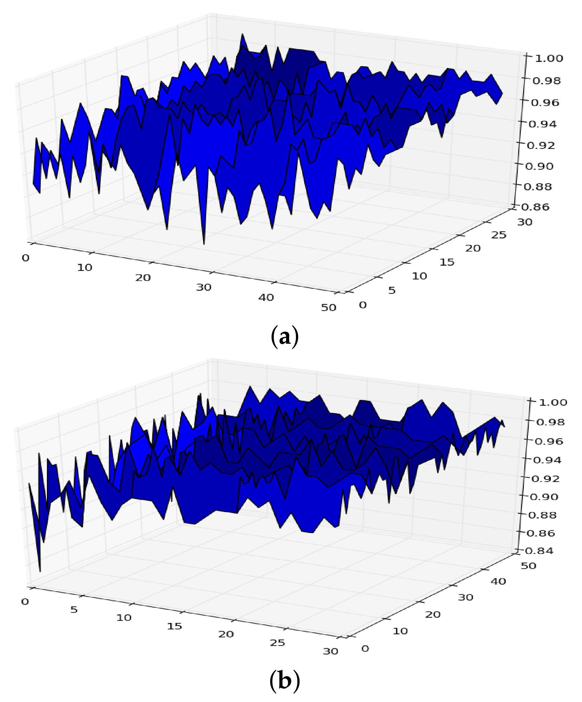
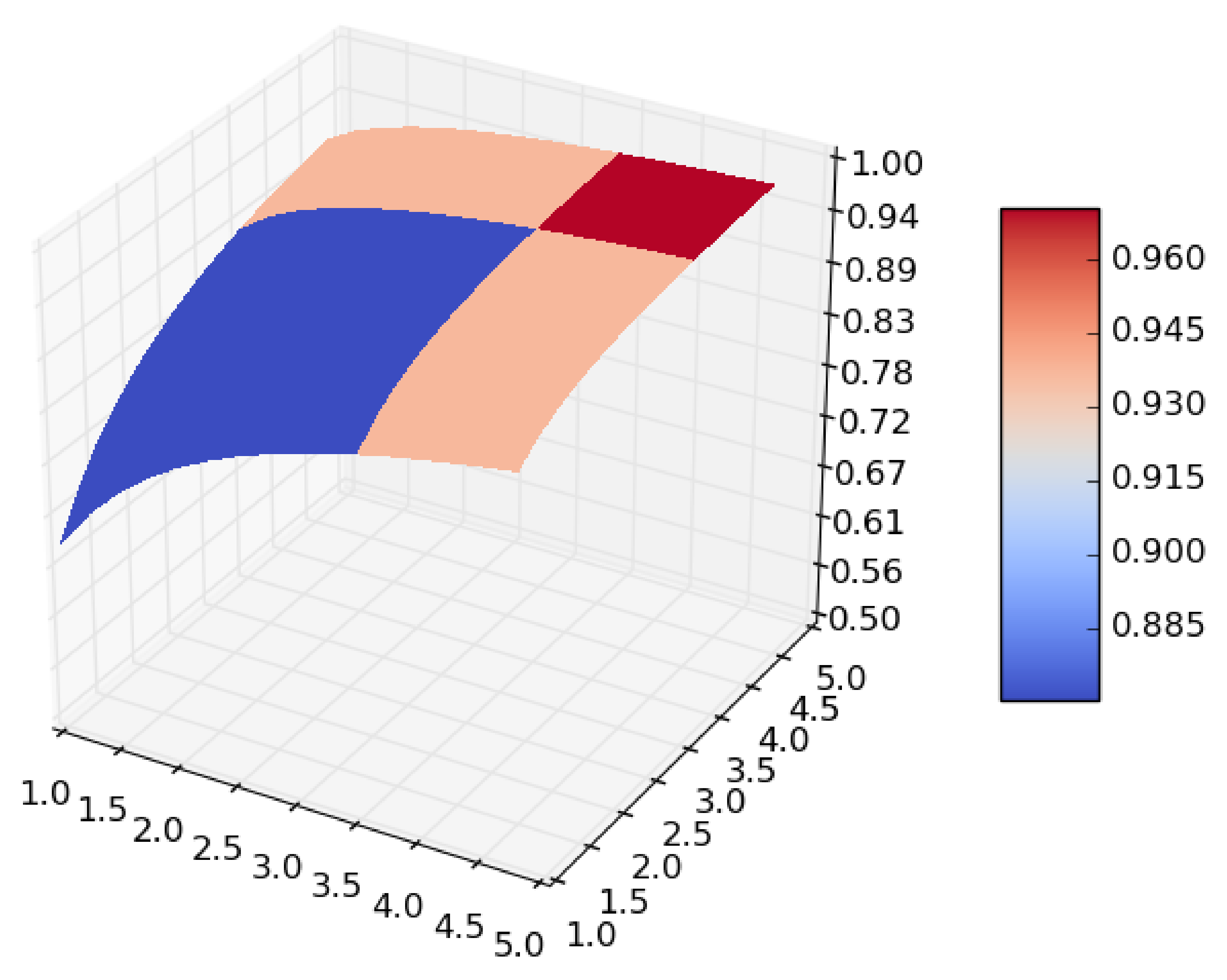
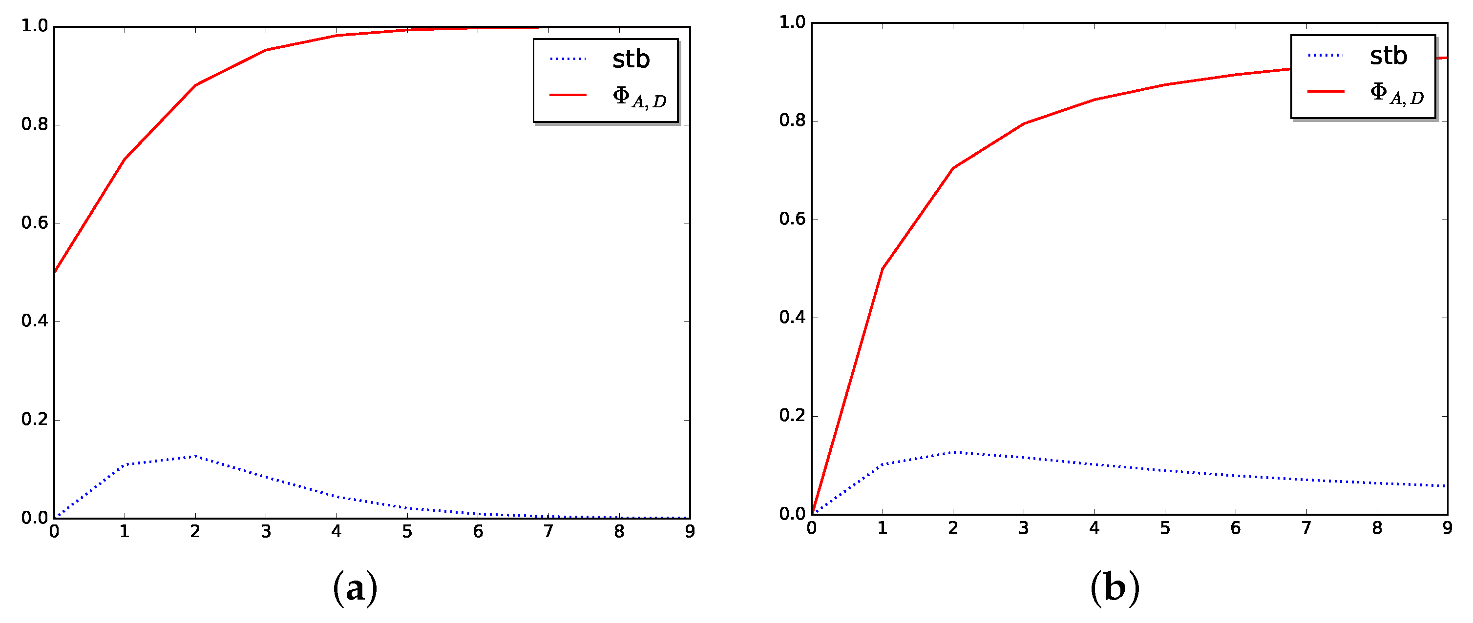
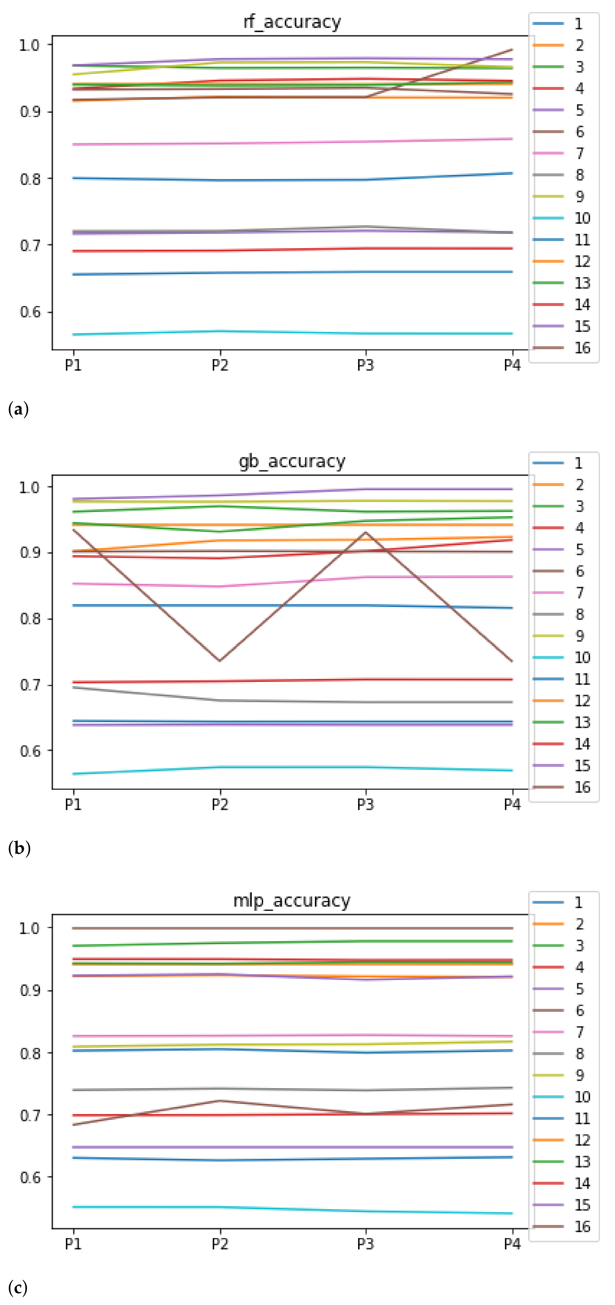
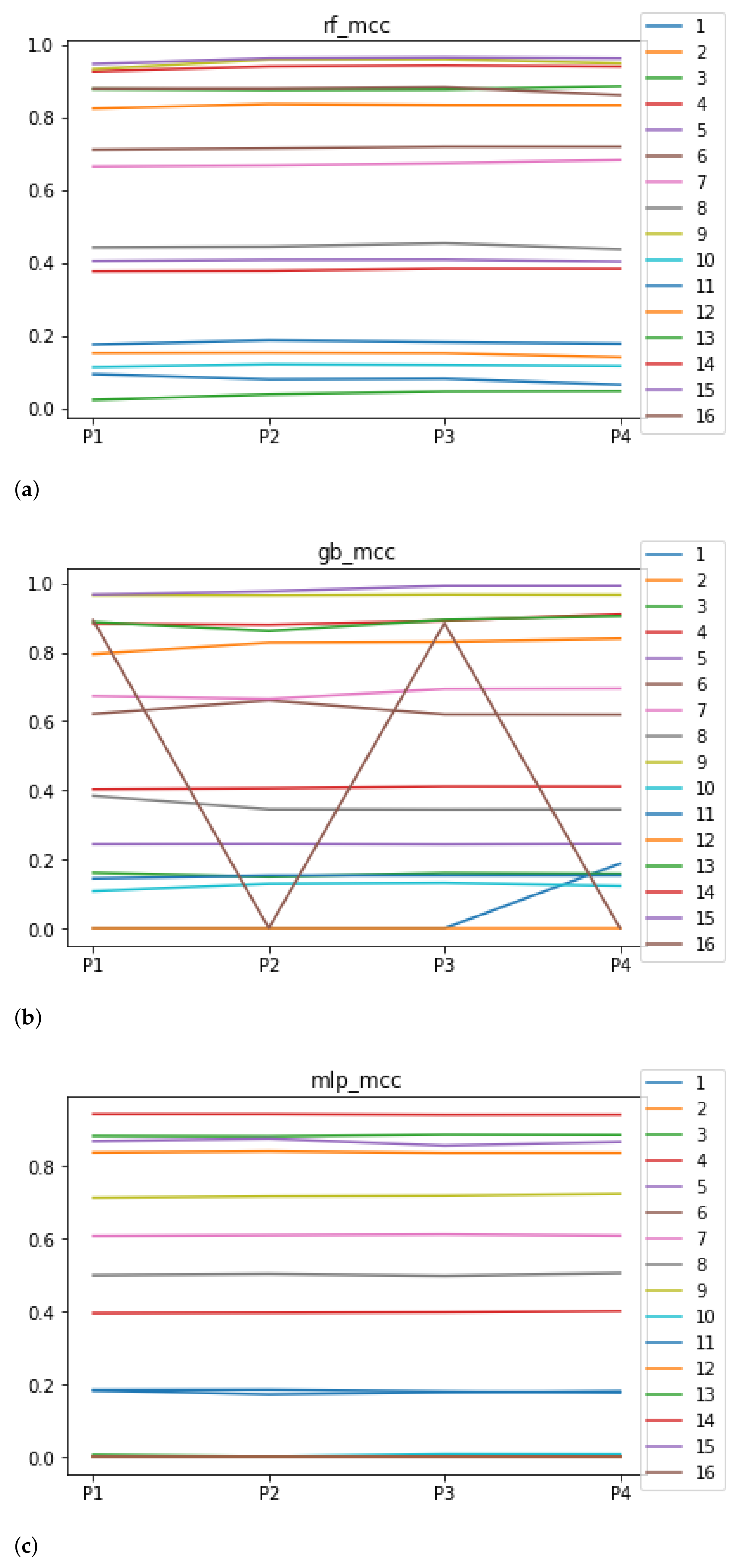
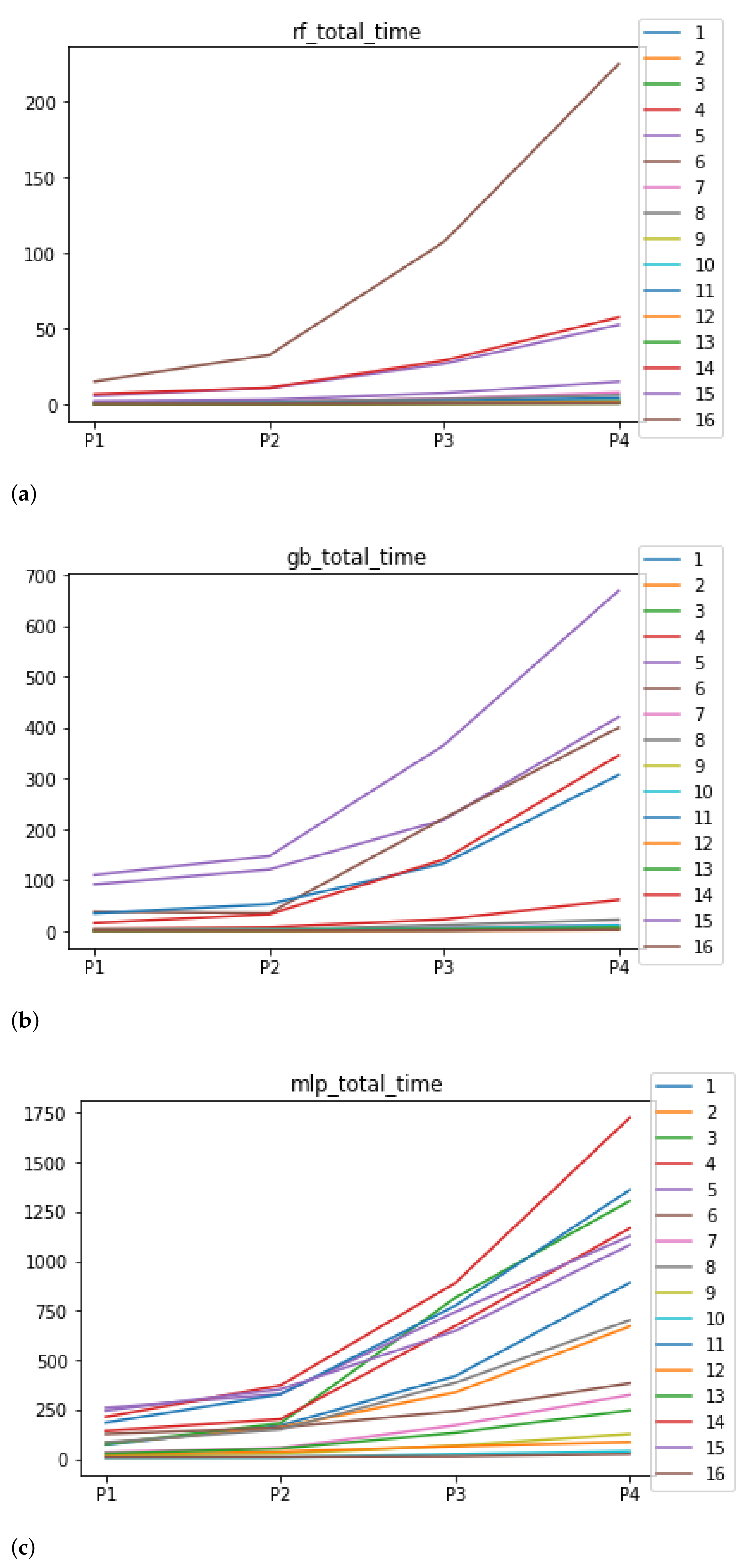
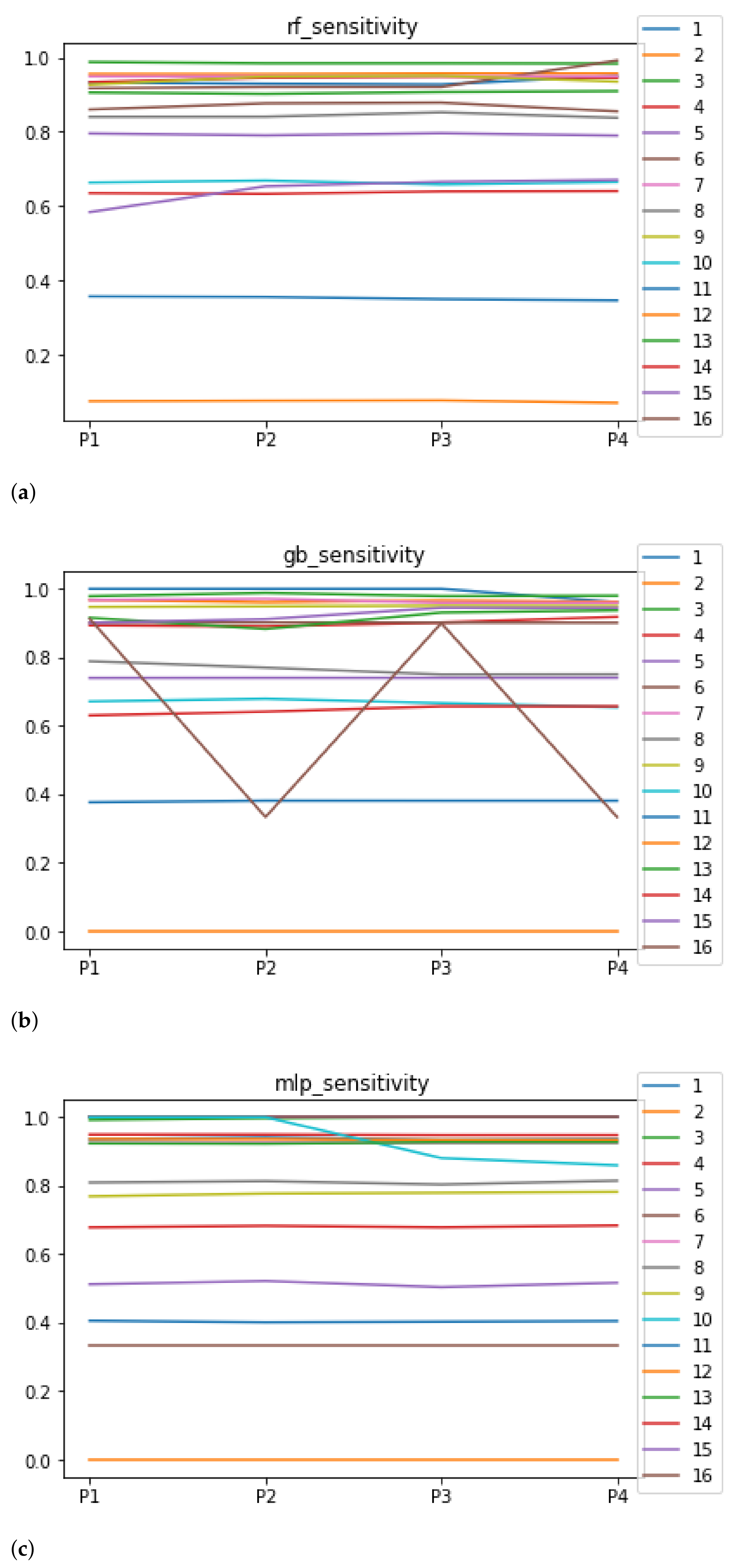
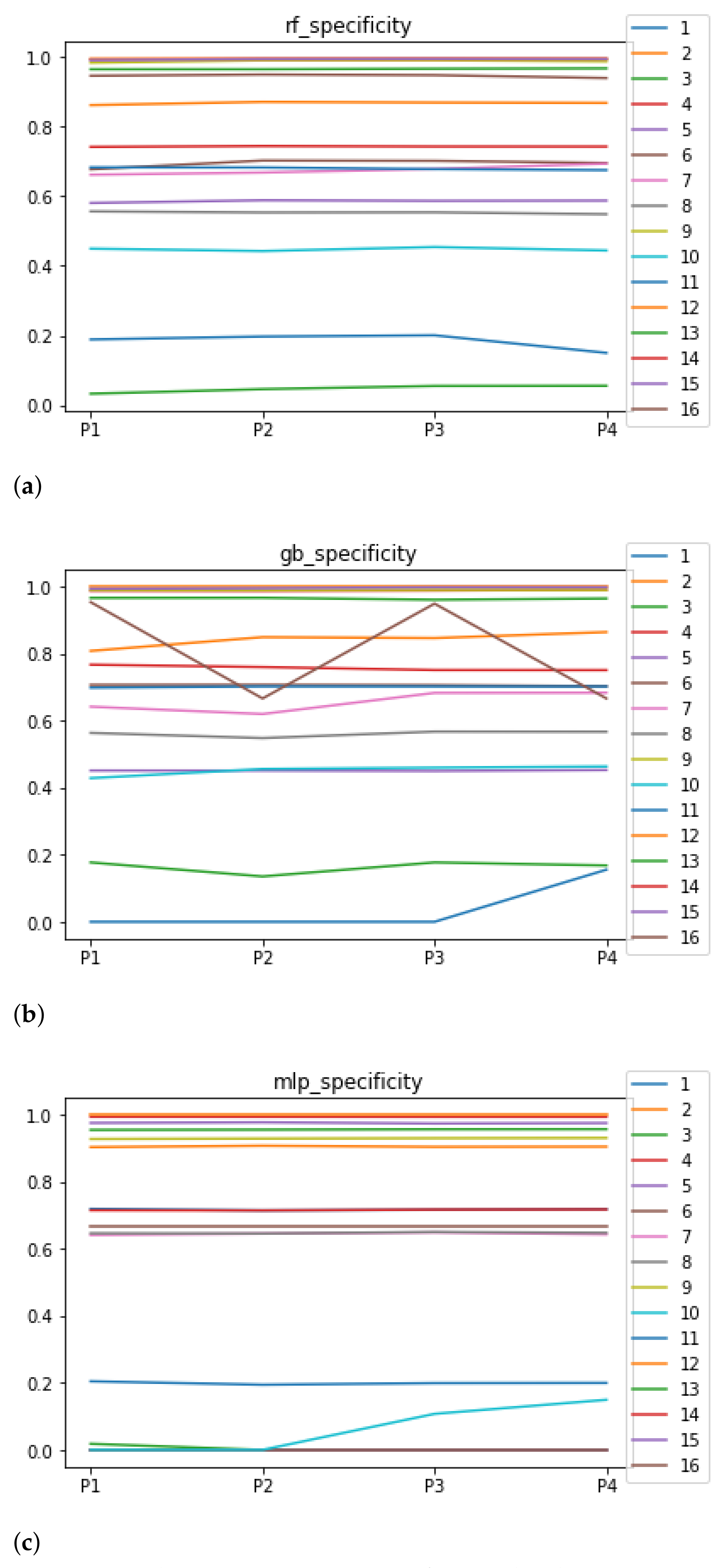
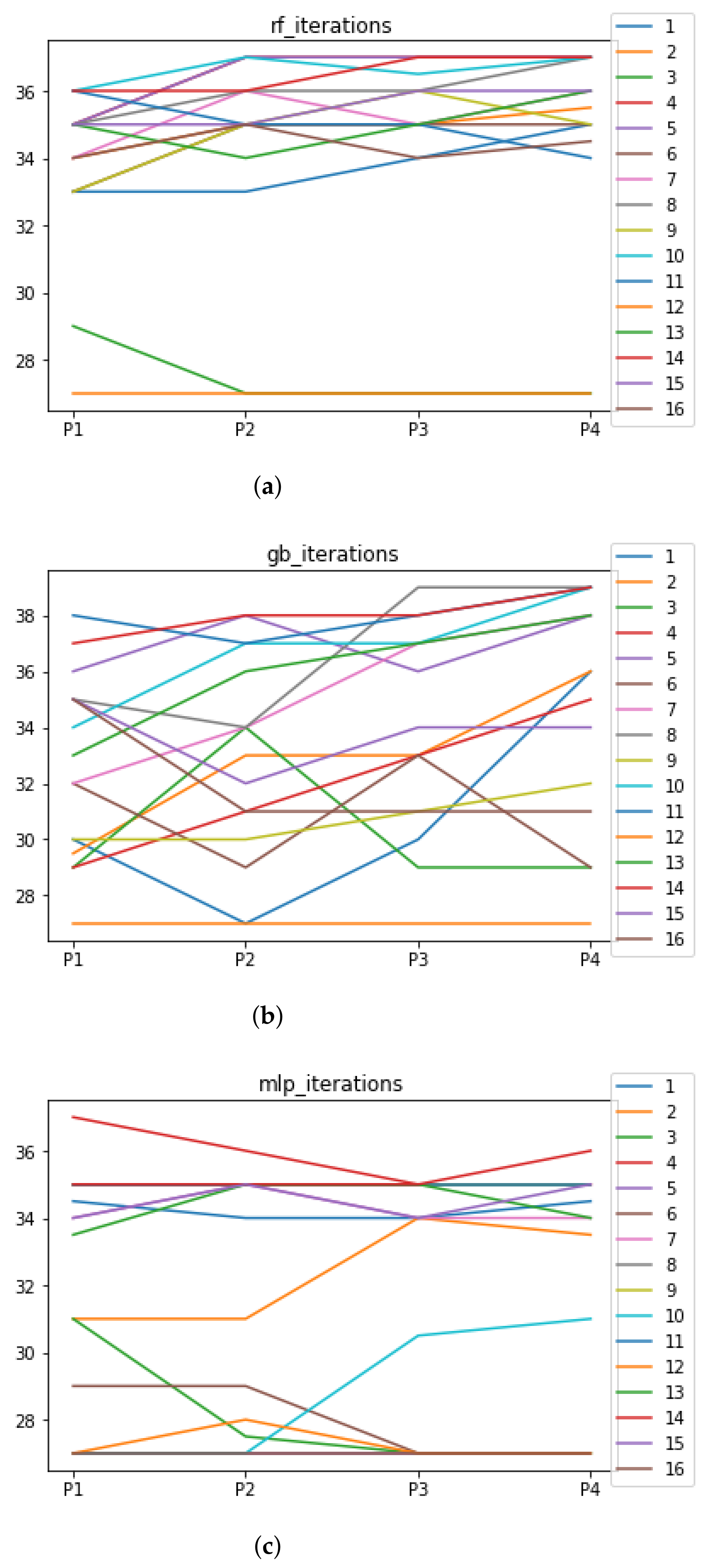
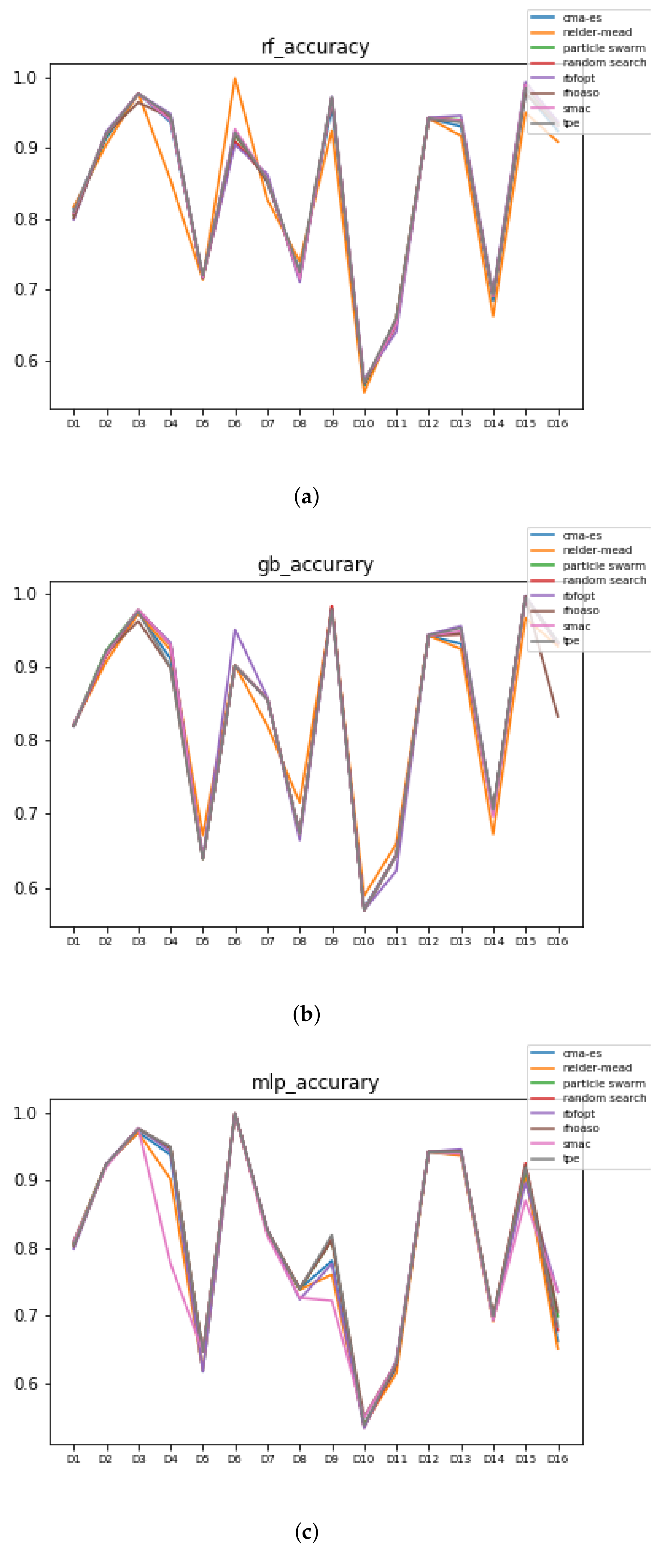
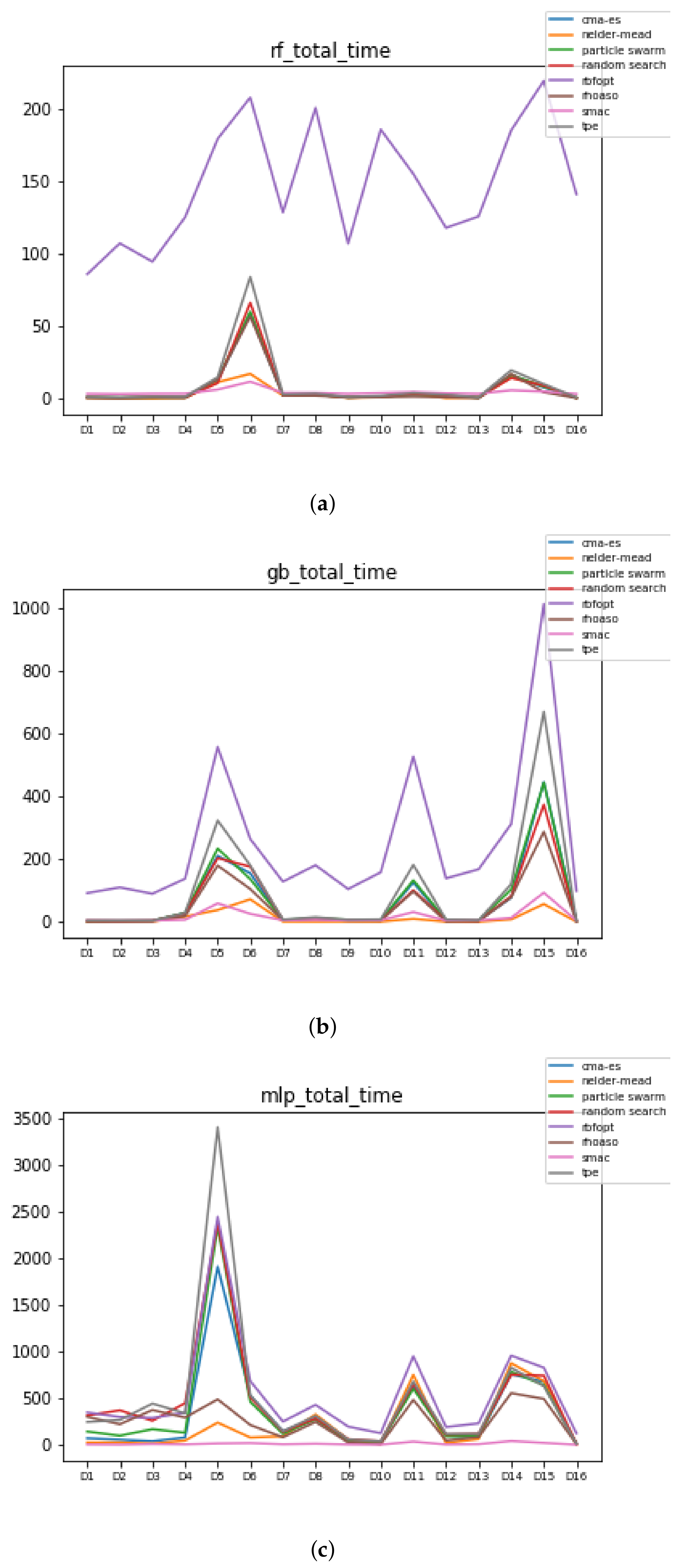
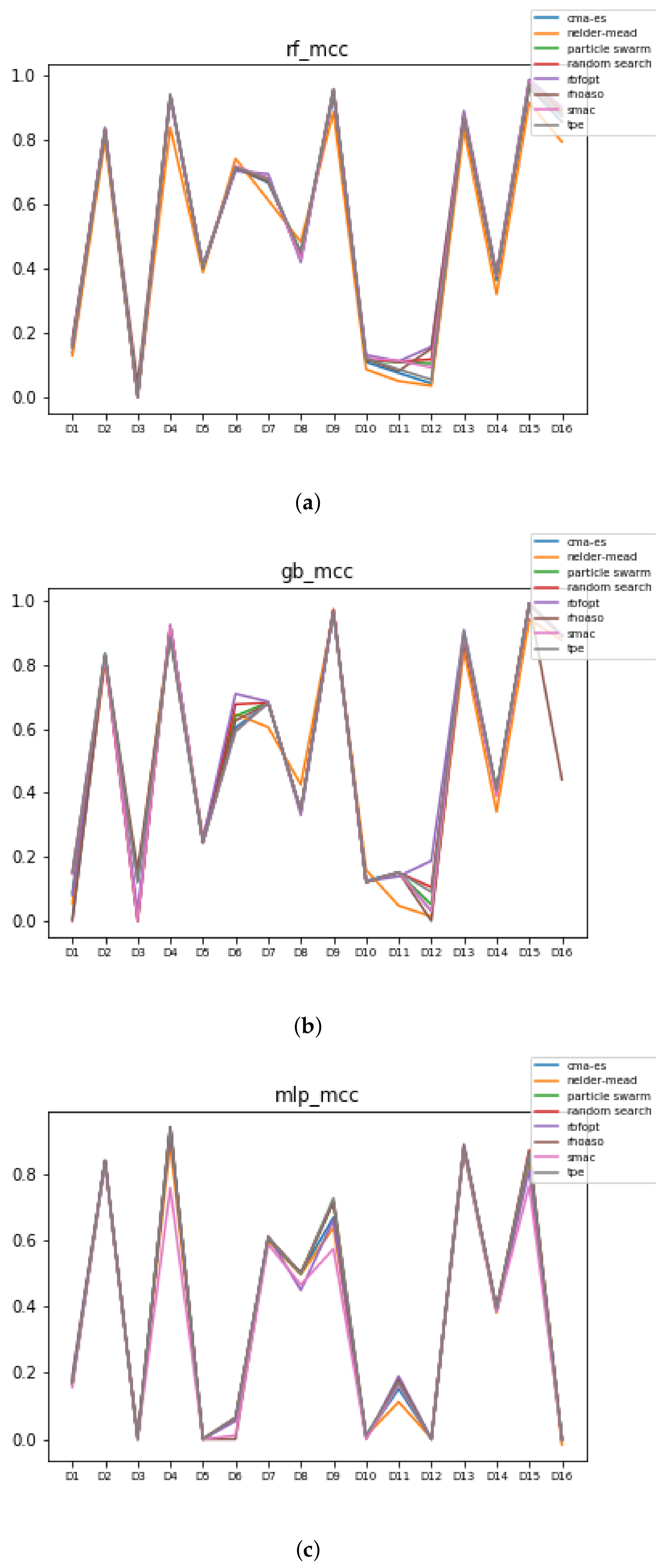
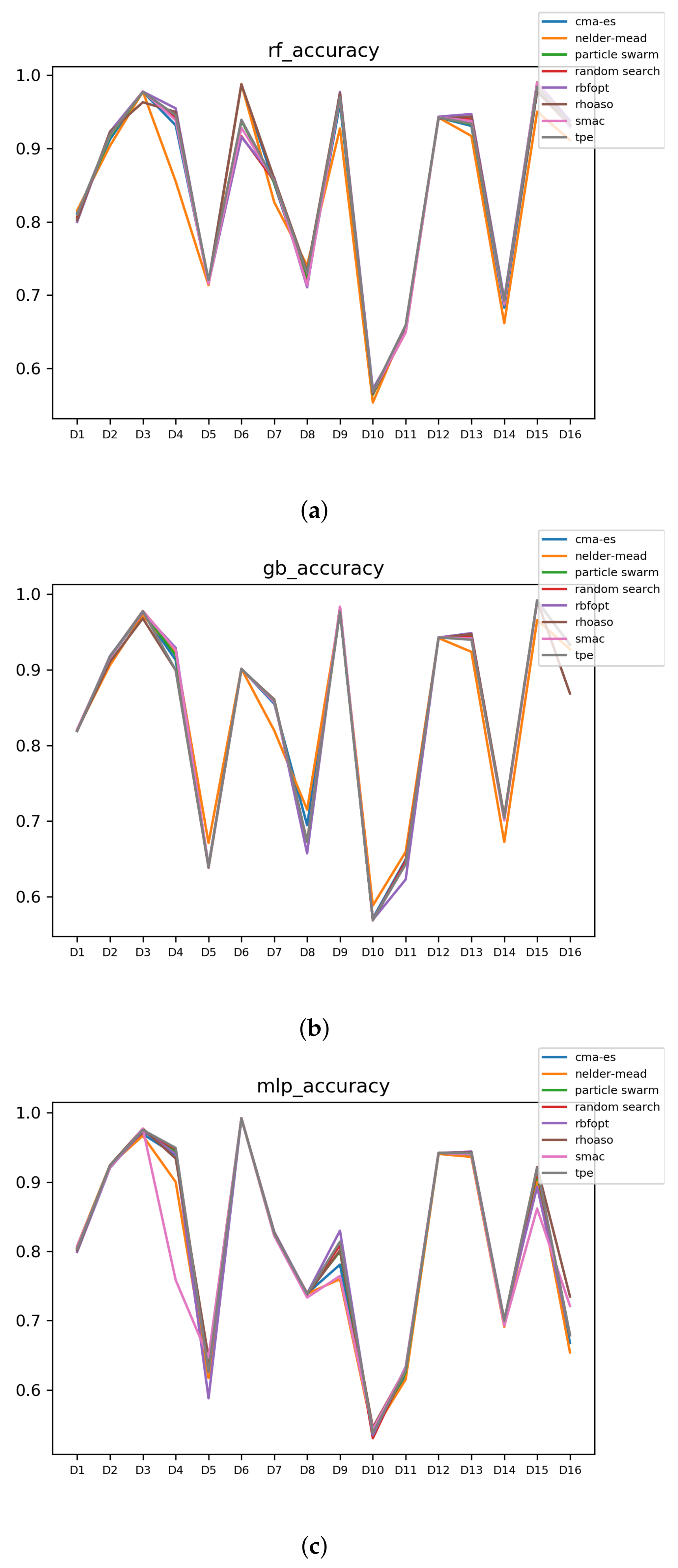
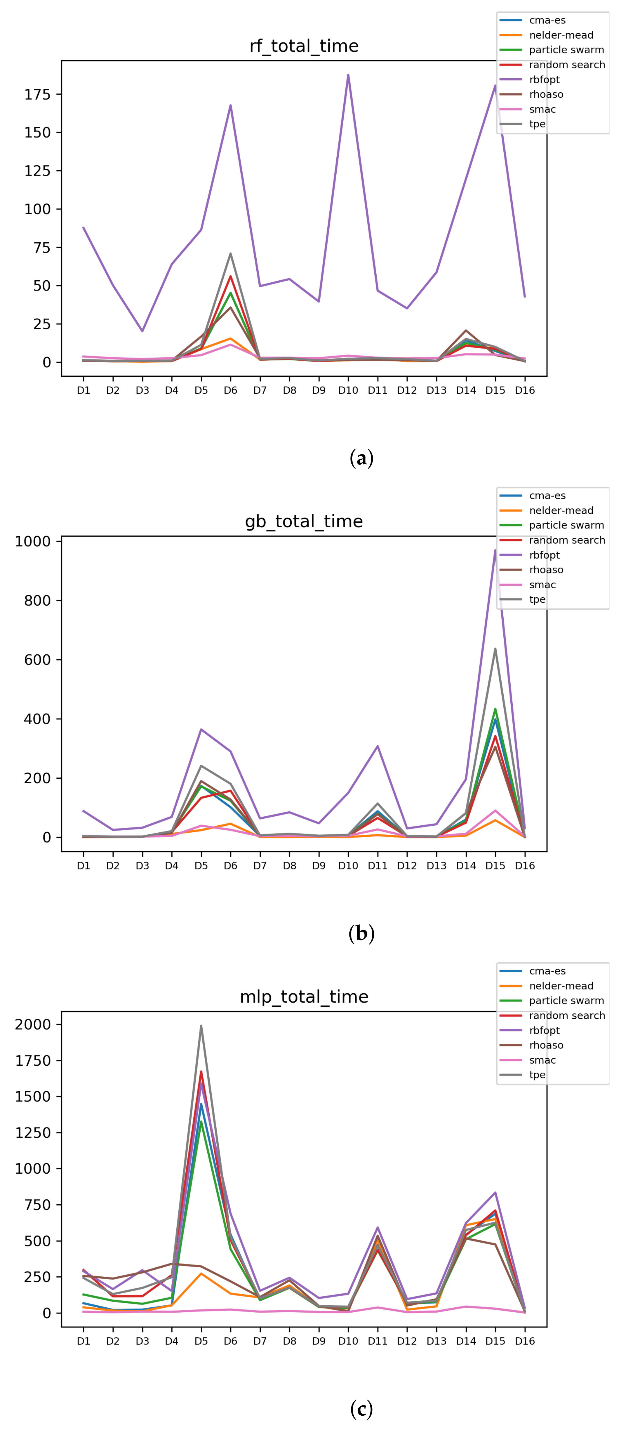
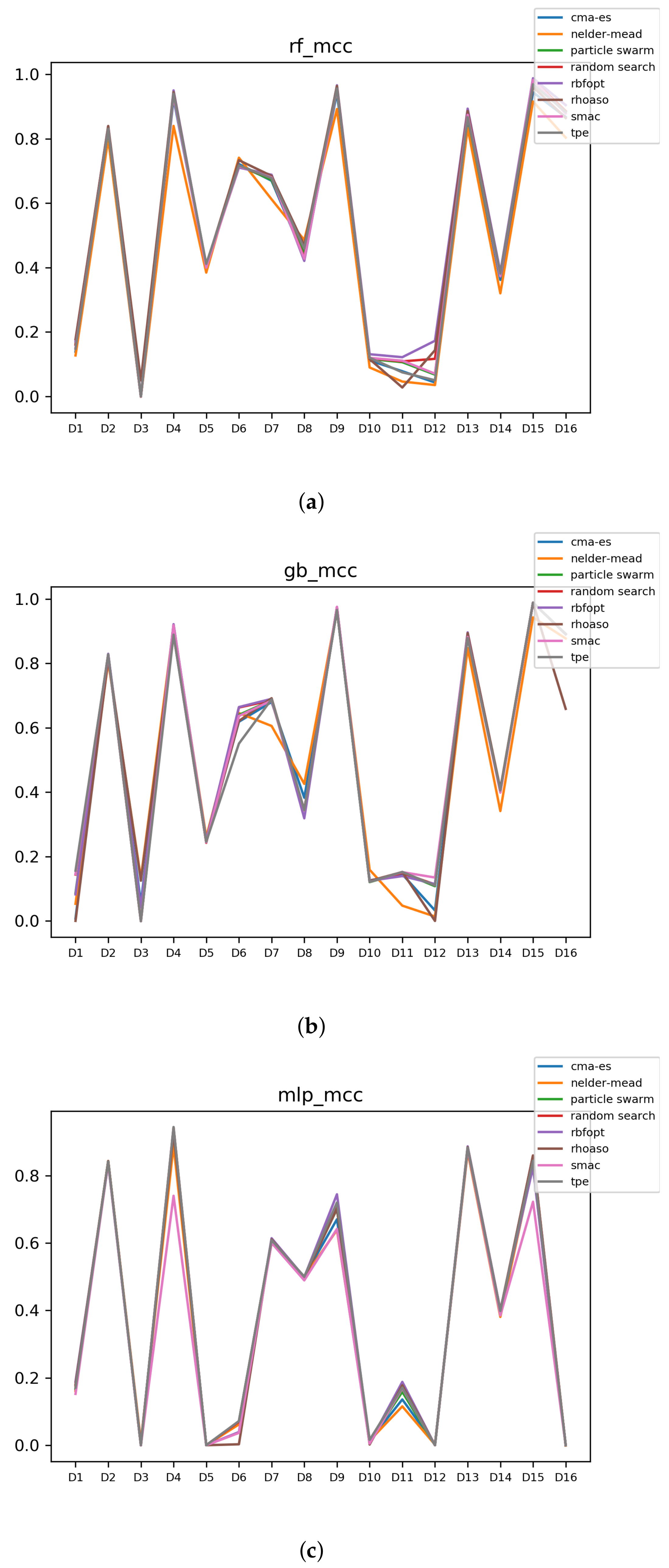
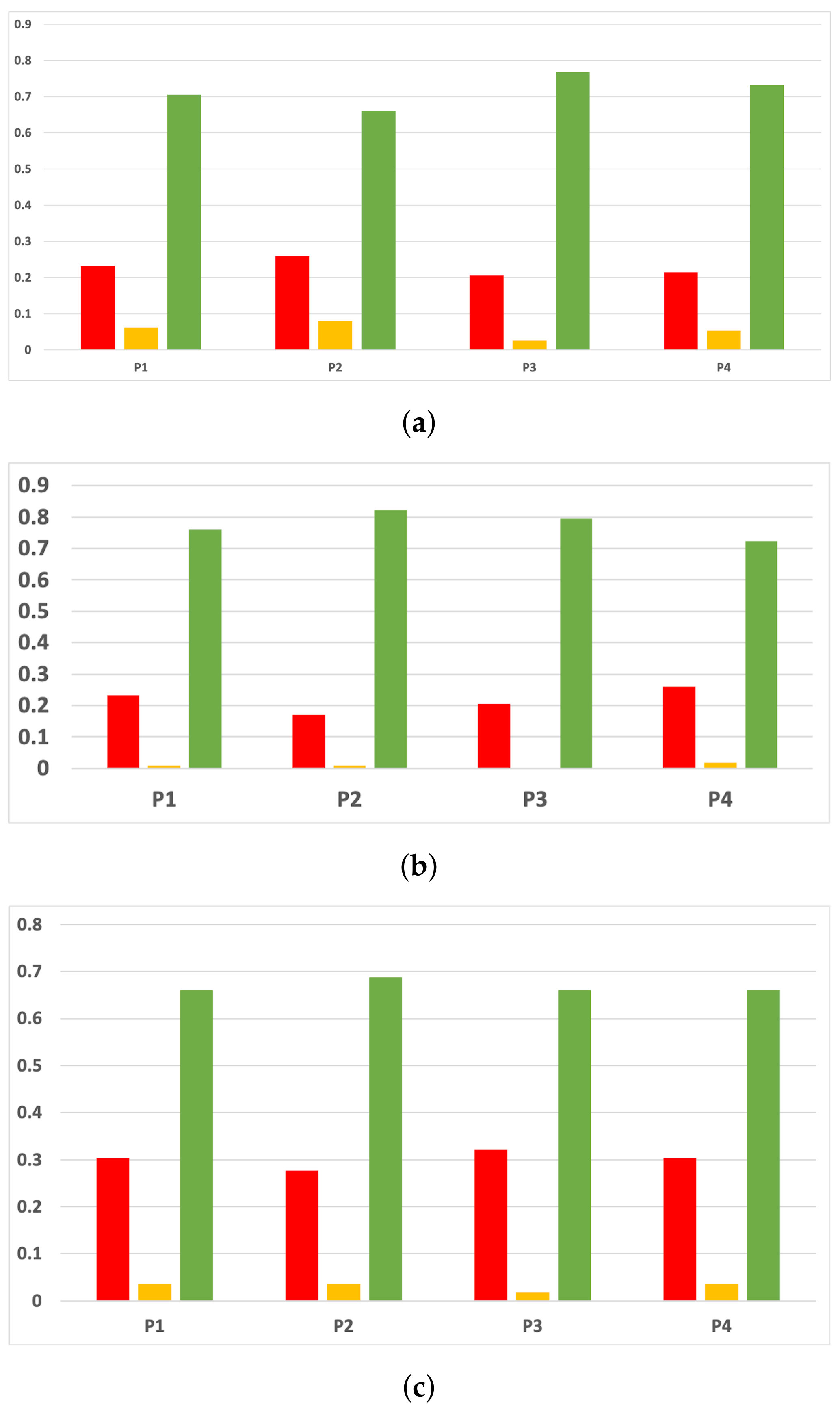
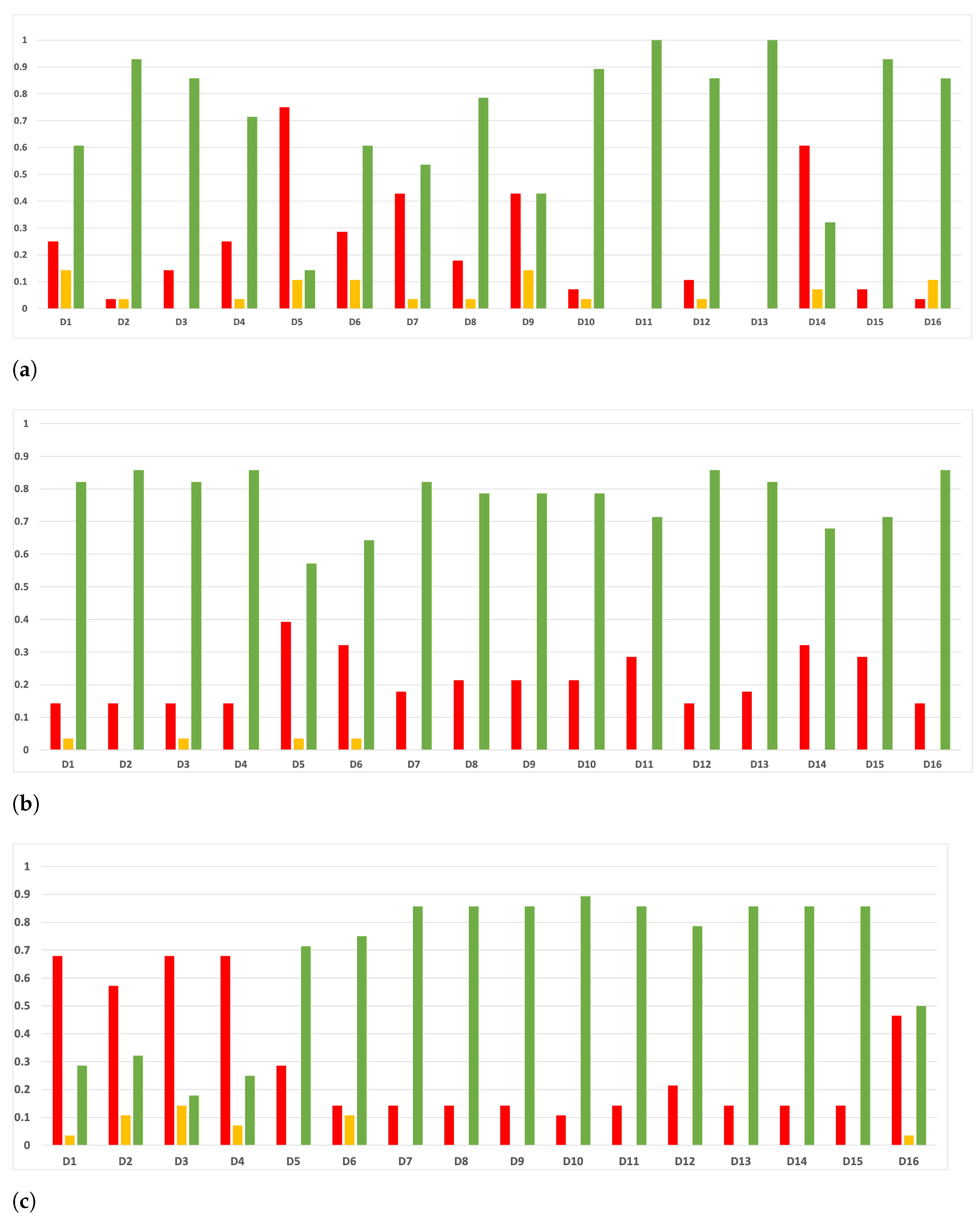
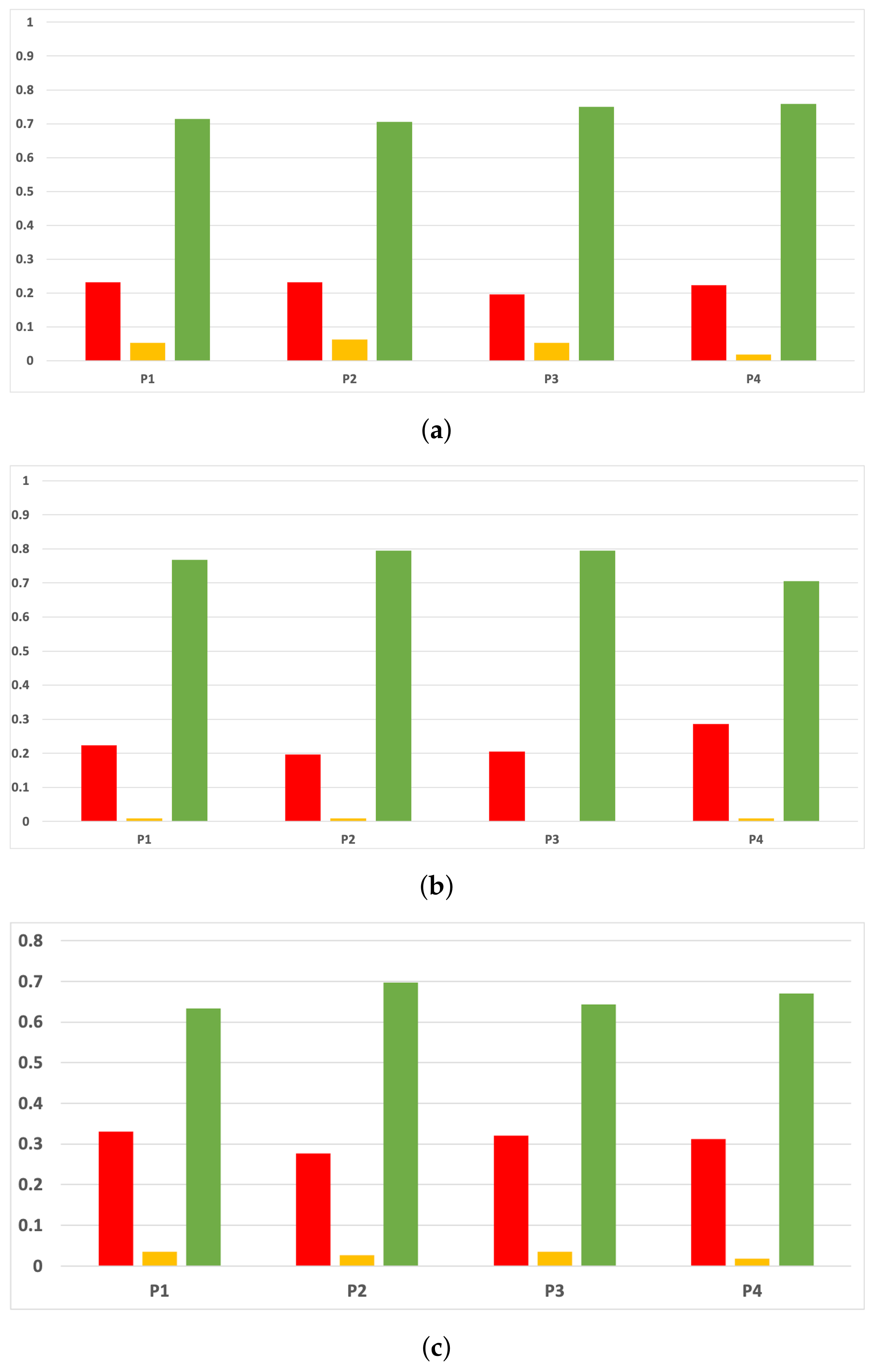
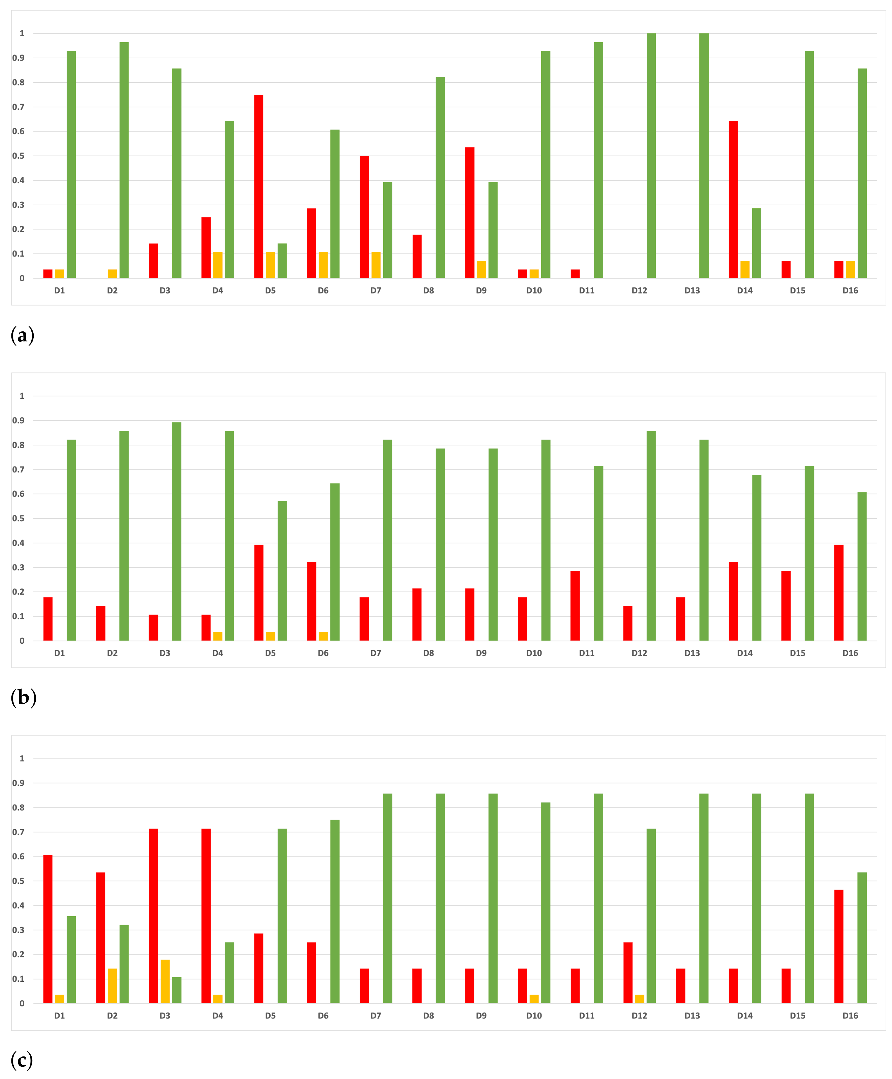
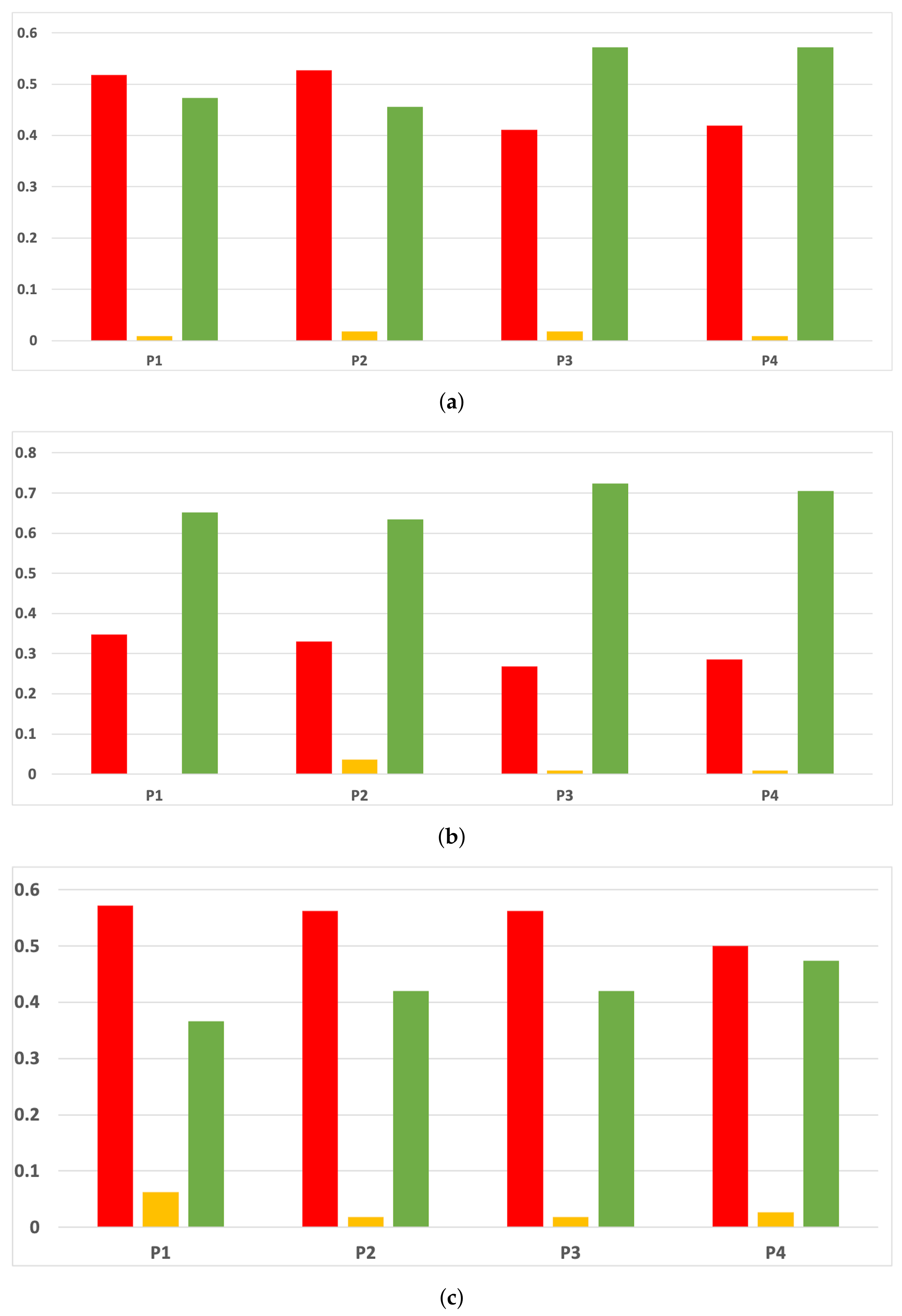
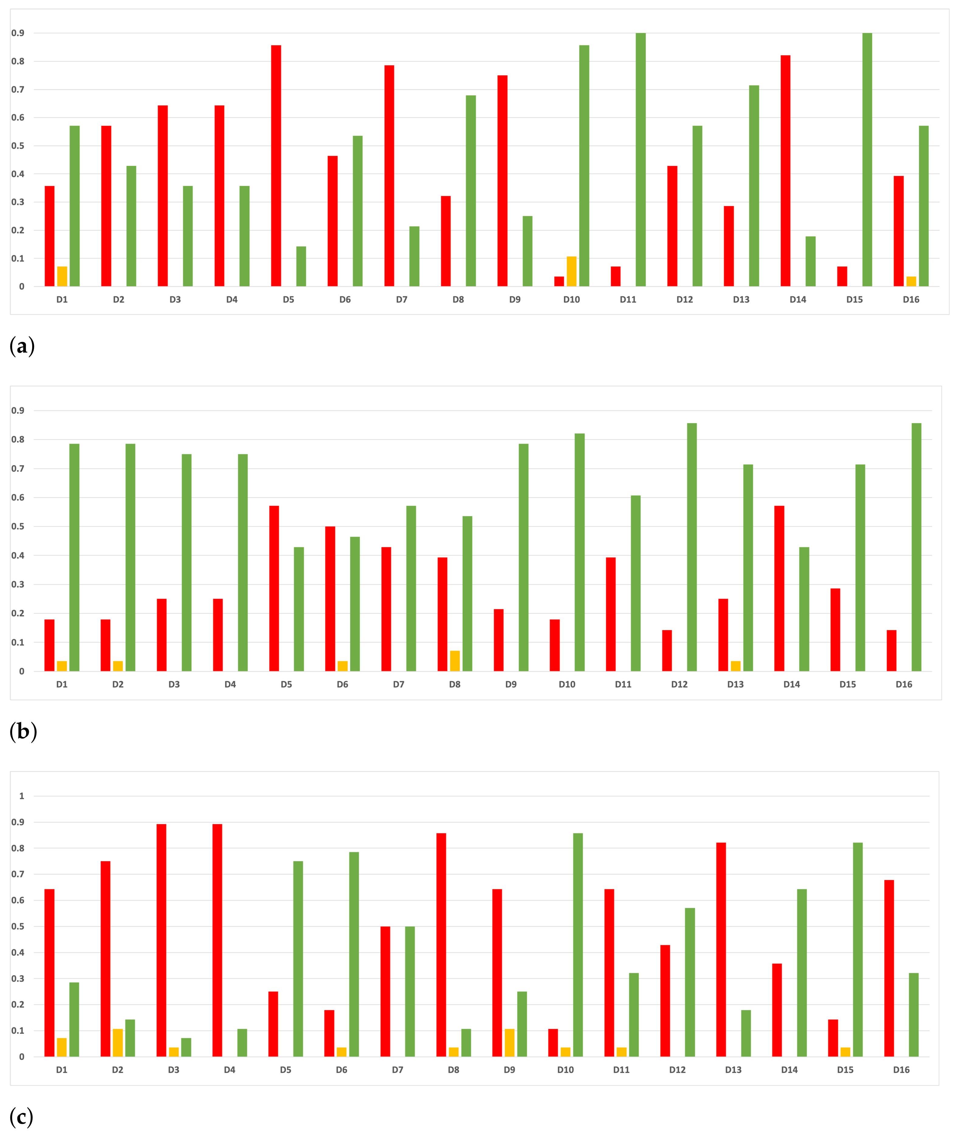
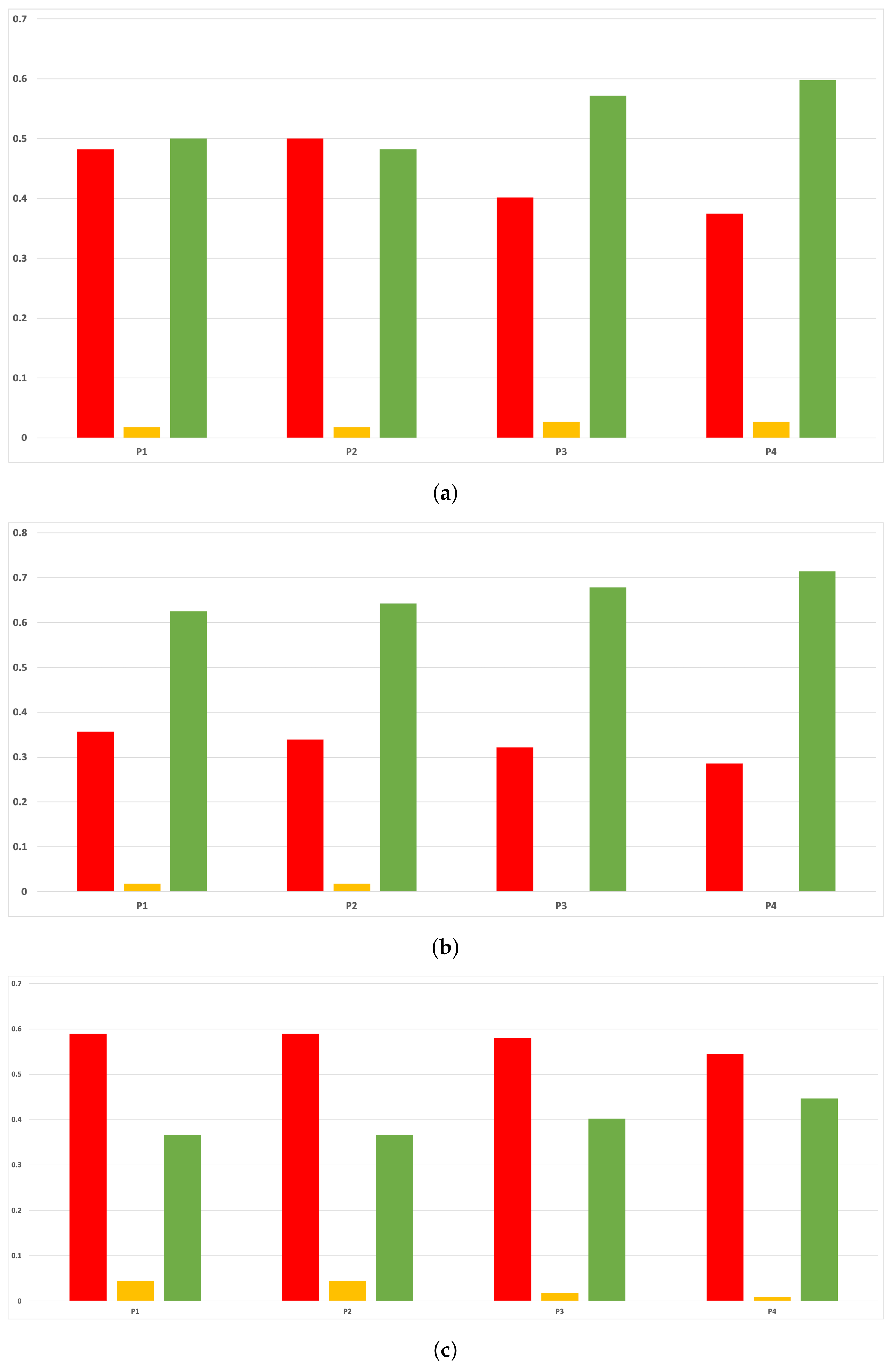

Publisher’s Note: MDPI stays neutral with regard to jurisdictional claims in published maps and institutional affiliations. |
© 2021 by the authors. Licensee MDPI, Basel, Switzerland. This article is an open access article distributed under the terms and conditions of the Creative Commons Attribution (CC BY) license (https://creativecommons.org/licenses/by/4.0/).