Convex Obstacles from Travelling Times

Abstract

We consider situations where rays are reflected according to geometrical optics by a set of unknown obstacles. The aim is to recover information about the obstacles from the travelling-time data of the reflected rays using geometrical methods and observations of singularities. Suppose that, for a disjoint union of finitely many strictly convex smooth obstacles in the Euclidean plane, no Euclidean line meets more than two of them. We then give a construction for complete recovery of the obstacles from the travelling times of reflected rays.

1. Introduction

For some $n\ge 1$, let $K_1,K_2,\dots ,K_n$ be disjoint closed convex subsets of Euclidean 2-space $E^2\cong {\mathbb{R}}^2$, with each boundary $\partial K_k$ a $C^{\infty }$ strictly convex Jordan curve. Let $K:={\cup }_{k=1}^n{K}_i$ be contained in the interior of the bounded component B of $E^2\backslash C$, where $C\subset E^2$ is also a strictly convex Jordan curve.

By a geodesic or, equivalently, a ray in the closure M of $E^2\backslash K$, we mean a piecewise-affine constant-speed curve $\gamma :\mathbb{R}\to M$ whose junctions are points of reflection on $\partial K$ with equal angles of incidence and reflection. The restriction of $\gamma$ to an interval is also called a geodesic. Given $x_0,x_1\in C$, the set of all geodesics $\gamma :[0,1]\to M$ with $\gamma \left(0\right)=x_0,\gamma \left(1\right)=x_1$ is denoted by ${\mathrm{\Gamma }}_{x_0,x_1}$. Then, $\gamma \in {\mathrm{\Gamma }}_{x_0,x_1}$ is critical for the length functional

$$J\left(x\right):={\int }_0^1\parallel \dot{x}\left(t\right)\parallel dt$$

over constant-speed piecewise-$C^1$ curves $x:[0,1]\to M$ satisfying $x\left(0\right)=x_0,x\left(1\right)=x_1$. We write

$$\mathrm{\Gamma }:={\cup }_{x_0,x_1\in C}{\mathrm{\Gamma }}_{x_0,x_1}.$$

Then, by Theorem 1.1 of [1], K is uniquely determined by its travelling-time data

$$\mathcal{T}:=\left\{\right(\gamma \left(0\right),\gamma \left(1\right),J\left(\gamma \right)):\gamma \in \mathrm{\Gamma }\}$$

namely by the travelling times of geodesics joining pairs of given points on C. Similar results are proved in [2] for obstacles in $E^m$ where $m>2$. Unfortunately, the proof of Theorem 1.1 in [1] is not constructive: all that is shown is that $\mathcal{T}$ is different for different convex obstacles K. When $n=1$, it is straightforward to calculate K from $\mathcal{T}$, and with a little more effort K can also be reconstructed when $n=2$ (see Section 4 in [3]). More interestingly, Theorem 1.1 of [4] allows the area of K to be computed from $\mathcal{T}$. Indeed, ref. [4] applies in a much more general setting, where the obstacles are not necessarily convex, and $E^2$ is replaced by a Riemannian manifold of any finite dimension. Importantly, the application of the result in [4] is made possible by the fact (proved in [1]) that the set of points generating trapped trajectories in the exterior of obstacles K considered in this paper has a Lebesgue measure of zero. Constructing K is equivalent to constructing $\partial K$, but this seems difficult for $n\ge 3$. We refer to [5,6] for general definitions and information about geodesic (billiard) flows on Riemannian manifolds. The present paper shows how to construct $\partial K$ from $\mathcal{T}$ when no line meets more than two connected components of K. Equivalently, K is required to satisfy Ikawa’s no-eclipse condition [7].

Inverse problems concerning metric rigidity have been studied for a long time in Riemannian geometry: we refer to [8,9,10,11] for more information. In the last 20 years or so similar problems have been considered for scattering by obstacles, where the task is to recover geometric information about an obstacle from its scattering length spectrum from travelling times of scattering rays in its exterior [3].

In general, an obstacle in Euclidean space $E^m\cong {\mathbb{R}}^m$ ($m\ge 2$) is a compact subset K of ${\mathbb{R}}^m$ with a smooth (e.g., $C^3$) boundary $\partial K$ such that ${\mathrm{\Omega }}_K=\overline{{\mathbb{R}}^m\backslash K}$ is connected. The scattering rays in ${\mathrm{\Omega }}_K$ are generalized geodesics (in the sense of Melrose and Sjöstrand [12,13,14]) that are unbounded in both directions. Most of these scattering rays are billiard trajectories with finitely many reflection points at $\partial K$ (there are no reflections at C). When K is a finite disjoint union of strictly convex domains, then all scattering rays in ${\mathrm{\Omega }}_K$ are billiard trajectories, namely geodesics of the type described above. We refer to [15,16,17,18] for general information about scattering theory and, in particular, for scattering by obstacles in Euclidean spaces.

It turns out that some kinds of obstacles are uniquely recoverable from their travelling-times spectra. For example, as mentioned above, this was proved in [2] for obstacles K in ${\mathbb{R}}^m$ ($m\ge 3$) that are finite disjoint unions of strictly convex bodies with $C^3$ boundaries. The case $m=2$ requires a different proof, given recently in [1].

The set of the so-called trapped points (points that generate trajectories with infinitely many reflections) plays a rather important role in various inverse problems in scattering by obstacles, and also in problems on metric rigidity in Riemannian geometry. As an example shown by M. Livshits (see e.g., Figure 1 in [19] or [4]), in general, the set of trapped points may contain a non-trivial open set. In such a case, the obstacle cannot be recovered from travelling times, because of an argument given in [4] due to Livshits based on the reflection properties of planar ellipses. In dimensions $m>2$ examples similar to that of Livshits are given in [19]. Other situations where geometric information cannot be recovered are studied in [20,21].

The layout of this paper is as folllows.

In Section 2, we collect some simple observations about linear (non-reflected) geodesics. This leads to the construction of $4(n^2-n)$, so-called vacuous arcs, ${\beta }_j$ in $\mathcal{T}$, and then $2(n^2-n)$ initial arcs in $\partial K$. Our plan is to build on the initial arcs, using travelling-time data from reflected rays to construct incremental arcs in $\partial K$, until eventually the whole of $\partial K$ is found. (Note however that, unlike the initial arcs, there are countably many incremental arcs, yielding diminishing additional information from ever-increasing amounts of precisely known data. In practice, insufficient data and limited computing power makes it difficult to carry out more than a few inductive steps, and $\partial K$ is found only approximately.) In Section 6 we describe an inductive step for constructing incremental arcs from previously determined arcs and from observations of $\mathcal{T}$. To make the relevant observations, we need to understand some of the mathematical structure of $\mathcal{T}$.

The first step towards this understanding is made in Section 3, where some simple facts about (typically non-reflected) geodesics are recalled. These facts, including a known result for computing initial directions of geodesics, are applied in Section 4 to investigate the structure of travelling-time data of nowhere-tangent geodesics. In particular, cusps in so-called echographs of $\mathcal{T}$ correspond to geodesics that are tangent to $\partial K$.

The family of all such cusps is studied in Section 5, where the augmented travelling-time data $\tilde{\mathcal{T}}$ are shown to be the closure of a countable family of disjoint open $C^{\infty }$ arcs ${\tilde{\beta }}_j$. As described in Section 6, the property of extendibility can be checked for each ${\tilde{\beta }}_j$. When ${\tilde{\beta }}_j$ is extendible, it yields an incremental arc in $\partial K$. When ${\tilde{\beta }}_j$ is not extendible, a trick using no-eclipse replaces ${\tilde{\beta }}_j$ by an extendible ${\tilde{\beta }}_{\overline{j}}$ yielding an incremental arc as previously described.

Although our methods are elementary, the construction is intricate, requiring numerous steps and different notations. A glossary of terms and notation is given as Table 1 at the end of this paper.

Table 1. Glossary of Terms and Notations.

Notation	Definition	Meaning
B	§1	known strictly convex set containing unknown obstacles
C	§1	boundary of B (strictly convex closed curve)
K	§1	union of unknown disjoint closed obstacles $K_i$
geodesic	§1	constant-speed piecewise-affine paths reflected by obstacles
$\mathrm{\Gamma }$	§1	all geodesics parameterised by $[0,1]$ from C to itself
$\mathcal{T}$	§1	travelling-time data (start, end, length) of geodesics in $\mathrm{\Gamma }$
no-eclipse	§1	a general-position condition
linear geodesics	§2	geodesics that are lines
${\mathcal{T}}_0$	§2	travelling-time data (ttd) of linear geodesics
$\tilde{\partial }{\mathcal{T}}_0$	§2	ttd of nontrivial linear geodesics
${\mathcal{T}}_0^q$	§2	ttd of q-times tangent linear geodesics
bitangent	§2	twice tangent linear geodesic
conjugate $\overline{j}$	§2	index of reverse of jth linear bitangent
${\mathrm{\Gamma }}^q$	§3	q-times tangent geodesics
${\mathcal{T}}^q$	§3	ttd from ${\mathrm{\Gamma }}^q$
${\gamma }_{x_0,v_0}$	§3	geodesic from $x_0$ with initial velocity $v_0$
$\mathcal{E}$	§3	endpoint map
order	§3	number of times geodesic meets K
$o\left(\gamma \right)$	§3	order of geodesic $\gamma$
${\mathrm{\Gamma }}_r$	§3	all order r geodesics
${\mathcal{T}}_{x_1}$	§4	ttd of geodesics ending at $x_1$
${\mathcal{T}}_{x_1}^q$	§4	ttd of q-times tangent geodesics ending at $x_1$
${\alpha }_{i,x_1}$	§4	open-bounded arcs whose union is ${\mathcal{T}}_{x_1}^0$
${\varphi }_i$	§4	generating function for ${\alpha }_i:={\alpha }_{i,x_1}$
echograph	§4	image of ${\mathcal{T}}_{x_1}$ under embedding $ϵ$
$\tilde{\mathcal{T}}$	§4	$\mathcal{T}$ augmented with initial directions
${\tilde{\mathcal{T}}}^q$	§4	${\mathcal{T}}^q$ augmented with initial directions
${\tilde{\mathcal{T}}}_{x_1}$	§4	${\mathcal{T}}_{x_1}$ augmented with initial directions
${\tilde{\mathcal{T}}}_{x_1}^q$	§4	${\mathcal{T}}_{x_1}^q$ augmented with initial directions
${\mathcal{T}}_{x_1}^{+}$	§5	${\mathcal{T}}_{x_1}^1\cup {\mathcal{T}}_{x_1}^2$
${\tilde{\mathcal{T}}}_{x_1}^{+}$	§5	${\tilde{\mathcal{T}}}_{x_1}^1\cup {\tilde{\mathcal{T}}}_{x_1}^2$
${\tilde{\mathcal{T}}}^{+}$	§5	${\tilde{\mathcal{T}}}^1\cup {\tilde{\mathcal{T}}}^2$
${\tilde{\beta }}_j$	§5	open arcs whose union is ${\tilde{\mathcal{T}}}^1$
bitangent	§5	geodesic tangent twice to $\partial K$
${\lambda }_j$	§5	smooth family of lines constructed from ${\tilde{\beta }}_j$
${\mathrm{\Lambda }}_{{\tilde{\beta }}_j}$	§5	envelope of ${\lambda }_j$
vacuous	§5	open arcs ${\tilde{\beta }}_j$ from linear tangential geodesics
extendible	§5	initial segments of geodesics for next arc $\tilde{\beta }$ are tangent

2. Linear Geodesics and Vacuous Arcs

From now on let $K={\cup }_{k=1}^n{K}_i$ be an obstacle in $E^2$, where $K_1,K_2,\dots ,K_n$ are disjoint closed convex subsets of $E^2$ with boundaries that are $C^{\infty }$ strictly convex Jordan curves. As before, assume that K is contained in the interior of the bounded component B of $E^2\backslash C$, where $C\subset E^2$ is also a strictly convex Jordan curve. We also assume that K satisfies no-eclipse. For the following lemma, it is not enough to require that a geodesic may not be tangent to $\partial K$ at more than two points. Nor is it sufficient to assume that a line in $E^2$ may not be tangent to $\partial K$ at more than 2 points. However, no-eclipse implies both these conditions, as is easily seen.

Lemma 1.

Geodesics in Γ are not tangent to $\partial K$, except perhaps at the first or last points of contact with $\partial K$ (either or both).

Proof. 

If tangency was at an intermediate point of contact, the tangent line would have common points with at least 3 connected components of K, contradicting no-eclipse. □

We begin by investigating travelling-times of linear geodesics, namely geodesics in $\mathrm{\Gamma }$ that do not reflect at all. The travelling-time data from linear geodesics can be obtained as follows:

$${\mathcal{T}}_0:=\mathcal{T}\cap \left\{\right(x_0,x_1,\parallel x_1-x_0\parallel ):x_0,x_1\in C\}\subset C\times C\times [0,\infty ).$$

Excluding points of the form $(x_0,x_0,0)\in \partial {\mathcal{T}}_0$, we obtain

$$\tilde{\partial }{\mathcal{T}}_0:=(C\times C\times (0,\infty ))\cap \partial {\mathcal{T}}_0={\cup }_{q\ge 1}{\mathcal{T}}_0^q$$

where ${\mathcal{T}}_0^q$ is defined as the travelling-time data from linear geodesics meeting $\partial K$ exactly q times tangentially and nowhere else. By Lemma 1, ${\mathcal{T}}_0^q=\varnothing$ for $q\ge 3$; namely ${\displaystyle \tilde{\partial }{\mathcal{T}}_0={\mathcal{T}}_0^1\cup {\mathcal{T}}_0^2}$. In the simplest case where $n=1$, ${\mathcal{T}}_0^2$ is empty, and $\partial K$ is constructed as the envelope of the smooth family $x_0\mapsto [x_0,x_1]$ of line segments, where $(x_0,x_1,\parallel x_1-x_0\parallel )\in \tilde{\partial }{\mathcal{T}}_0$. Suppose $n\ge 2$ from now on.

Proposition 1.

${\mathcal{T}}_0^1$ is a union of $4(n^2-n)$ nonintersecting bounded open $C^{\infty }$ arcs ${\beta }_j$ whose boundaries in $\tilde{\partial }{\mathcal{T}}_0$ comprise ${\mathcal{T}}_0^2$, which is finite of size $4(n^2-n)$.

Proof. 

For $1\le k\ne k^{\prime }\le n$ there are 8 directed Euclidean line segments (linear bitangents) tangent to both $\partial K_k$ and $\partial K_{k^{\prime }}$. Each directed linear bitangent is an endpoint of two maximal open arcs of directed line segments that are singly tangent. The travelling-time data for the linear bitangents are ${\mathcal{T}}_0^2$. The travelling-time data for the open arcs ${\beta }_j$ are the path components of ${\mathcal{T}}_0^1$. □

Therefore, n is found from ${\mathcal{T}}_0^1$.

Definition 1.

For $1\le j\le 4(n^2-n)$ the conjugate $\overline{j}$ is defined to be $j+2(n^2-n)$ or $j-2(n^2-n)$ according as $1\le j\le 2(n^2-n)$ or $2(n^2-n)+1\le j\le 4(n^2-n)$.

Evidently $\overline{\overline{j}}=j$. Order the arcs ${\beta }_j$ in ${\mathcal{T}}_0^1$ so that $(x_0,x_1,t)\in {\beta }_j\iff (x_1,x_0,t)\in {\beta }_{\overline{j}}$. The initial arcs in $\partial K$ are the $2(n^2-n)$ nonempty disjoint connected open subsets of $\partial K$ found as the envelopes of the $[x_0,x_1]$, where $(x_0,x_1,t)\in {\beta }_j$ for $1\le j\le 2(n^2-n)$. For each $1\le k\le n$ there are $2(n-1)$ initial arcs in $\partial K_k$.

3. Nonlinear Geodesics

Define ${\mathrm{\Gamma }}^q$ to be the space of geodesics $\gamma \in \mathrm{\Gamma }$ that are tangent exactly q times to $\partial K$. The corresponding travelling-time data are denoted by ${\mathcal{T}}^q$. Most nonlinear geodesics are nowhere-tangent; namely, they lie in ${\mathrm{\Gamma }}^0$. Their travelling-time data will be used to construct $C^{\infty }$ travelling-time functions ${\varphi }_i$ for Lemma 3, as needed for Propositions 3, 4 of §4.

Whereas ${\mathcal{T}}_0^1$ is found by simple inspection of $\mathcal{T}$, some effort is required to isolate ${\mathcal{T}}^1$, which is needed to construct envelopes of nonlinear singly tangential geodesics. We recall some known results about directions of geodesics and travelling times.

For $(x_0,v_0)\in (E^2-K)\times {\mathbb{R}}^2$ let ${\gamma }_{(x_0,v_0)}:\mathbb{R}\to M$ be the geodesic satisfying ${\gamma }_{(x_0,v_0)}\left(0\right)=x_0$ and ${\dot{\gamma }}_{(x_0,v_0)}\left(0\right)=v_0$. The endpoint map $\mathcal{E}:(E^2-K)\times E^2\to M$ is the continuous function given by $\mathcal{E}(x_0,v_0):={\gamma }_{(x_0,v_0)}\left(1\right)$. Then, $\parallel v_0\parallel$ is the length of the restriction ${\gamma }_{x_0,v_0}|[0,1]$. Although $\mathcal{E}$ is continuous, it is not differentiable at points $(x_0,v_0)$, where ${\gamma }_{x_0,v_0}$ is tangent to $\partial K$.

Lemma 2.

For $x_0\in E^2-K$, suppose that ${\gamma }_{(x_0,v_0)}|[0,1]$ is nowhere tangent to $\partial K$, and that ${\gamma }_{(x_0,v_0)}\left(1\right)\notin \partial K$. Then $\mathcal{E}$ is smooth near $(x_0,v_0)\in (E^2-K)\times E^2$, and the restriction of its derivative $d{\mathcal{E}}_{x_0,v_0}:{\mathbb{R}}^2\times {\mathbb{R}}^2\to {\mathbb{R}}^2$ to $\left\{\mathbf{0}\right\}\times {\mathbb{R}}^2$ is a linear isomorphism.

Proof. 

For variable perturbations ${\tilde{v}}_0=e^{\mathbf{i}h}{v}_0$ of $v_0$ with $\left|h\right|$ sufficiently small, the ${\gamma }_{x_0,{\tilde{v}}_0}|[0,1]$ are also nowhere-tangent to $\partial K$. Here we identify ${\mathbb{R}}^2$ with ℂ in the standard way. Considering the effects of repeated reflections of the ${\gamma }_{x_0,{\tilde{v}}_0}|[0,1]$, we find by routine calculation that the regular $C^{\infty }$ parameterised curve

$$h\mapsto {\gamma }_{x_0,{\tilde{v}}_0}\left(1\right)=\mathcal{E}(x_0,{\tilde{v}}_0)$$

meets the geodesic ${\gamma }_{x_0,v_0}$ transversally at ${\gamma }_{x_0,v_0}\left(1\right)=\mathcal{E}(x_0,v_0)$; namely, $d{\mathcal{E}}_{x_0,v_0}(\mathbf{0},\mathbf{i}{v}_0)$ is not a multiple of ${\dot{\gamma }}_{x_0,v_0}\left(1\right)$. For variable perturbations $(1+h)v_0$ of $v_0$ where $\left|h\right|$ is small, the curve

$$h\mapsto {\gamma }_{x_0,(1+h)v_0}\left(1\right)=\mathcal{E}(x_0,(1+h)v_0)$$

is a geodesic. Indeed, a reparameterisation of part of ${\gamma }_{x_0,v_0}$ with velocity ${\dot{\gamma }}_{x_0,v_0}\left(1\right)$ at $h=0$. Therefore, $d{\mathcal{E}}_{x_0,v_0}(\mathbf{0},v_0)={\dot{\gamma }}_{x_0,v_0}\left(1\right)$ and $d{\mathcal{E}}_{x_0,v_0}(\mathbf{0},\mathbf{i}{v}_0)$ are linearly independent. □

Lemma 3.

For $x_0\ne x_1:=\mathcal{E}(x_0,v_0)$ and with the hypotheses of Lemma 2, there exists an open neighbourhood $U_0$ of $x_0$ in $E^2-K$, and a unique $C^{\infty }$ function $\varphi :={\varphi }_{x_0,v_0}:U_0\to (0,\infty )$ whose gradient $\nabla \varphi$ is everywhere of unit length, satisfying

$$\mathcal{E}({\tilde{x}}_0,-\varphi \left({\tilde{x}}_0\right)\nabla \varphi \left({\tilde{x}}_0\right))=x_1$$

for all ${\tilde{x}}_0\in U_0$. Here $\varphi \left(x_0\right)=\parallel v_0\parallel$ with $\nabla \varphi \left(x_0\right)=-v_0/\parallel v_0\parallel$.

Proof. 

By Lemma 2 and the implicit function theorem, there exist a unique $C^{\infty }$ function $X:U_0\to E^2$ satisfying $\mathcal{E}({\tilde{x}}_0,X\left({\tilde{x}}_0\right))=x_1$ for all ${\tilde{x}}_0\in U_0$. Because $x_0\ne x_1$, X is never-zero for $U_0$ sufficiently small. Then the geodesic ${\gamma }_{({\tilde{x}}_0,X\left({\tilde{x}}_0\right))}:[0,1]\to M$ joining ${\tilde{x}}_0,x_1$, has length

$${\displaystyle \varphi \left({\tilde{x}}_0\right):=\parallel X\left({\tilde{x}}_0\right)\parallel =J\left(x_{({\tilde{x}}_0,X\left({\tilde{x}}_0\right))}\right).}$$

Differentiating with respect to ${\tilde{x}}_0\in U_0$ in the direction of $\delta \in R^2$, we find $d{\varphi }_{{\tilde{x}}_0}\left(\delta \right)=-⟨X\left({\tilde{x}}_0\right)/\parallel X\left({\tilde{x}}_0\right)\parallel ,\delta ⟩$, because geodesics are critical for J when variations have fixed endpoints. □

The order $o\left(\gamma \right)$ of a geodesic $\gamma$ is the number of intersections with $\partial K$. Write

$${\mathrm{\Gamma }}_r:=\{\gamma \in \mathrm{\Gamma }:o\left(\gamma \right)=r\}.$$

Let $d_K$ be the minimum distance between obstacles. Writing $\tau \left(\gamma \right):=t$ for the travelling time (length) of $\gamma \in \mathrm{\Gamma }$,

$$o\left(\gamma \right)d_K\le J\left(\gamma \right)\le o\left(\gamma \right)\mathrm{diam}\left(C\right).$$

(1)

4. Arcs and Generators for Nowhere-Tangent Geodesics

Recall that ${\mathrm{\Gamma }}_r$ is the space of geodesics that intersect $\partial K$ precisely r times, and that ${\mathrm{\Gamma }}^q$ is the space of geodesics $\gamma \in \mathrm{\Gamma }$ that are exactly q-times tangent to $\partial K$. Because of no-eclipse and Lemma 1, ${\mathrm{\Gamma }}^q$ is empty for $q\ge 3$. Set

$${\mathcal{T}}^q:=\{(\gamma \left(0\right),\gamma \left(1\right),J\left(\gamma \right)):\gamma \in {\mathrm{\Gamma }}^q\}\subset \mathcal{T}.$$

Recall that ${\mathcal{T}}_0^q$ is the travelling-time data from geodesics meeting $\partial K$ exactly q times tangentially, and nowhere else. Then, ${\mathcal{T}}_0^q\subset {\mathcal{T}}^q$ and ${\mathcal{T}}^q=\varnothing$ for $q\ge 3$. We have shown how to construct ${\mathcal{T}}_0^q$, but not yet ${\mathcal{T}}^q$ from $\mathcal{T}$ for $q\le 2$.

For $x_1\in C$ define

$${\mathcal{T}}_{x_1}:=\{(x_0,t):(x_0,x_1,t)\in \mathcal{T}\}\subset C\times \mathbb{R},{\mathcal{T}}_{x_1}^q:=\{(x_0,t):(x_0,x_1,t)\in {\mathcal{T}}^q\}\subset {\mathcal{T}}_{x_1}.$$

Likewise ${\mathrm{\Gamma }}_{x_1}\subset \mathrm{\Gamma }$ is the set of geodesics $\gamma :[0,1]\to M$ with $\gamma \left(1\right)=x_1$. Set

$${\mathrm{\Gamma }}_{x_1}^q:={\mathrm{\Gamma }}_{x_1}\cap {\mathrm{\Gamma }}^q.$$

Although ${\mathcal{T}}_{x_1}$ is found directly from the given travelling-time data $\mathcal{T}$, we have yet to show how ${\mathcal{T}}_{x_1}^q$ is found from $\mathcal{T}$ for $q=0,1,2$ (this is done in the paragraph following Corollary 1 below).

It is easily seen that ${\mathcal{T}}_{x_1}^0$ is open and dense in ${\mathcal{T}}_{x_1}$, that ${\mathcal{T}}^1$ is open and dense in $\mathcal{T}\backslash {\mathcal{T}}^0={\mathcal{T}}^1\cup {\mathcal{T}}^2$, and that ${\mathcal{T}}^2$ is discrete.

Proposition 2.

${\mathcal{T}}_{x_1}^2$ has at most $2n$ elements, and is empty for $x_1$ in an open dense subset of C.

Proof. 

By Lemma 1, the first and last segments of any $\gamma \in {\mathrm{\Gamma }}_{x_1}^2$ are tangent to $\partial K$. Because $\partial K$ is strictly convex, there are at most $2n$ such geodesics. Therefore, ${\mathcal{T}}_{x_1}^2$ has a size at most of $2n$. A small perturbation of $x_1$ causes a $C^{\infty }$ perturbation of the last points of tangency of $\gamma$, destroying the first points of tangency, by strict convexity. □

Proposition 3.

For $x_1\in C$, we have ${\mathcal{T}}_{x_1}^0={\cup }_{i\ge 1}{\alpha }_{i,x_1}$, where

1.

the ${\alpha }_i:={\alpha }_{i,x_1}$ are countably many pairwise-transversal $C^{\infty }$ open bounded arcs in $C\times R$,

2.

${\cup }_{q\ge 1}{\mathcal{T}}_{x_1}^q={\cup }_{i\ge 1}\partial {\alpha }_i$,

3.

each ${\alpha }_i$ has a generator, namely a $C^{\infty }$ function ${\varphi }_i:U_i\to R$ with $U_i\subset E^2$ open, such that

• $U_i\cap C$ is an open arc in C, and ${\tilde{x}}_0\mapsto ({\tilde{x}}_0,{\varphi }_i\left({\tilde{x}}_0\right))$ is a diffeomorphism from $U_i\cap C$ onto ${\alpha }_i$,
• ${\gamma }_{({\tilde{x}}_0,{\nu }_i\left(x_0\right))}|[0,1]\in {\mathrm{\Gamma }}_{x_1}^0$, where ${\nu }_i\left({\tilde{x}}_0\right):=-{\varphi }_i\left({\tilde{x}}_0\right)\nabla {\varphi }_i\left({\tilde{x}}_0\right)$ for ${\tilde{x}}_0\in U_i\cap C$.

Proof. 

For $(x_0,t)\in {\mathcal{T}}_{x_1}^0$, there exists $\gamma \in {\mathrm{\Gamma }}_{x_1}$ with $J\left(\gamma \right)=t$. Then, $x_1=\mathcal{E}(x_0,v_0)$, where $v_0=\dot{\gamma }\left(0\right)$. By Lemma 3, for some open neighbourhood $U_0$ of $x_0$ in $E^2$, there is a unique $C^{\infty }$ function $\varphi ={\varphi }_{x_0,v_0}:U_0\to (0,\infty )$ with $\varphi \left(x_0\right)=t$ and $\nabla {\varphi }_{x_0}=-v_0/\parallel v_0\parallel$, such that $\mathcal{E}({\tilde{x}}_0,-\varphi \left({\tilde{x}}_0\right)\nabla \varphi \left({\tilde{x}}_0\right))=x_1$ for all ${\tilde{x}}_0\in U_0$. In particular, the last equation holds for ${\tilde{x}}_0\in U_0\cap C$; namely, ${\tilde{x}}_0\mapsto ({\tilde{x}}_0,\varphi \left({\tilde{x}}_0\right))$ embeds $U_0\cap C$ in ${\mathcal{T}}_{x_1}^0$. By continuation, the embedding extends uniquely in both directions around C, until just before $\gamma$ is tangent to some $\partial K_k$, which must eventually happen. Therefore, ${\mathcal{T}}_{x_1}^0$ is a countable union of $C^{\infty }$ embedded arcs ${\alpha }_i$.

Pairwise transversality is proved by contradiction as follows. Suppose ${\alpha }_i\ne {\alpha }_{i^{\prime }}$ meet tangentially at $(x_0,t)\in {\mathcal{T}}_{x_1}^0$. Then $⟨\nabla {\varphi }_{x_0,v_i}\left(x_0\right),w⟩=⟨\nabla {\varphi }_{x_0,v_{i^{\prime }}}\left(x_0\right),w⟩$ where $\parallel v_i\parallel =t=\parallel v_{i^{\prime }}\parallel$, and $w\ne \mathbf{0}$ is tangent to C at $x_0$. By Lemma 3, $\nabla {\varphi }_{x_0,v_i}\left(x_0\right)$ and $\nabla {\varphi }_{x_0,v_{i^{\prime }}}\left(x_0\right)$ point out from the bounded component B of $E^2\backslash C$ at $x_0$. Therefore, $-v_i=t\nabla {\varphi }_{x_0,v_i}\left(x_0\right)=t\nabla {\varphi }_{x_0,v_{i^{\prime }}}\left(x_0\right)=-v_{i^{\prime }}$ by Lemma 3, contradicting ${\alpha }_i\ne {\alpha }_{i^{\prime }}$.

Because ${\mathcal{T}}_{x_1}^0$ is open and dense in ${\mathcal{T}}_{x_1}$, ${\cup }_{q\ge 1}{\mathcal{T}}_{x_1}^q={\cup }_{i\ge 1}\partial {\alpha }_i$. □

By continuity, the orders $o\left({\alpha }_i\right)$ of the ${\gamma }_{({\tilde{x}}_0,{\nu }_i\left({\tilde{x}}_0\right))}\in {\mathrm{\Gamma }}^0$ are independent of ${\tilde{x}}_0\in U_i\cap C$. From (1) we obtain, for all ${\tilde{x}}_0\in U_i\cap C$,

$$o\left({\alpha }_i\right)d_K\le {\varphi }_i\left({\tilde{x}}_0\right)\le o\left({\alpha }_i\right)\mathrm{diam}\left(C\right),$$

(2)

and the arcs ${\alpha }_i$ are similarly bounded. For any i, the closures ${\overline{\alpha }}_i$ and ${\overline{\alpha }}_{i^{\prime }}$ in ${\mathcal{T}}_{x_1}$ are disjoint for all but finitely many $i^{\prime }$, where $i,i^{\prime }\ge 1$. The generator ${\varphi }_i$ defines ${\gamma }_{({\tilde{x}}_0,{\nu }_i\left({\tilde{x}}_0\right))}\in {\mathrm{\Gamma }}_{x_1}^0$ for every ${\tilde{x}}_0\in U_i\cap C$. For $(x_0,t)\in \partial {\alpha }_i$, define

$${\nu }_i\left(x_0\right):={\lim }_{{\tilde{x}}_0\to x_0}{\nu }_i\left({\tilde{x}}_0\right)\in E^2.$$

Then ${\gamma }_{(x_0,{\nu }_i\left(x_0\right))}\in {\mathrm{\Gamma }}_{x_1}^1\cup {\mathrm{\Gamma }}_{x_1}^2$, and $(x_0,t)\in {\mathcal{T}}_{x_1}^1\cup {\mathcal{T}}_{x_1}^2$ where $t=\parallel {\nu }_i\left(x_0\right)\parallel$.

Proposition 4.

If $(x_0,t)\in {\mathcal{T}}_{x_1}^1$ then $\left\{(x_0,t)\right\}=(\partial {\alpha }_i)\cap (\partial {\alpha }_{i^{\prime }})$ for some unique $i,i^{\prime }$ with $o\left({\alpha }_{i^{\prime }}\right)=o\left({\alpha }_i\right)+1$. Then $U_i\cap C$ and $U_{i^{\prime }}\cap C$ are on the same side of $x_0$ in C and, for ${\tilde{x}}_0\in U_i\cap U_{i^{\prime }}\cap C$, ${\varphi }_{i^{\prime }}\left({\tilde{x}}_0\right)>{\varphi }_i\left({\tilde{x}}_0\right)$. We also have

$$\underset{{\tilde{x}}_0\to x_0}{lim}{\varphi }_i\left({\tilde{x}}_0\right)=\underset{{\tilde{x}}_0\to x_0}{lim}{\varphi }_{i^{\prime }}\left({\tilde{x}}_0\right)=t,\underset{{\tilde{x}}_0\to x_0}{lim}\nabla {\varphi }_i\left({\tilde{x}}_0\right)=\underset{{\tilde{x}}_0\to x_0}{lim}\nabla {\varphi }_{i^{\prime }}\left({\tilde{x}}_0\right).$$

Proof. 

Write $t=J\left(\gamma \right)$, where $\gamma \in {\mathrm{\Gamma }}_{x_1}^1$ has length t and $\gamma \left(0\right)=x_0$. Suppose the last (respectively first) segment of $\gamma$ is not tangent to $\partial K$. Then, by no-eclipse, the first (last) segment is tangent. Perturbing the last segment while maintaining the endpoint $x_1$ gives two arcs of nowhere-tangent geodesics, whose initial points ${\tilde{x}}_0$ lie on the same side of $x_0$ in C. Along one arc, the first (last) segment remains linear and the order decreases by 1. Along the other arc, the first (last) segment breaks into two linear segments, maintaining the order and increasing the travelling-time.

Write $v_0=\dot{\gamma }\left(0\right)$. For ${\tilde{x}}_0$ near $x_0$, the two arcs of geodesics define arcs $\left\{({\tilde{x}}_0,{\varphi }_i\left({\tilde{x}}_0\right))\right\}$, $\left\{({\tilde{x}}_0,{\varphi }_{i^{\prime }}\left({\tilde{x}}_0\right))\right\}$ in ${\mathcal{T}}_{x_1}^0$ contained in maximal arcs ${\alpha }_i,{\alpha }_{i^{\prime }}$, labelled so that $o\left({\alpha }_{i^{\prime }}\right)=o\left({\alpha }_i\right)+1$. Then ${\nu }_{i^{\prime }}\left(x_0\right)=v_0={\nu }_i\left(x_0\right)$, and ${\varphi }_{i^{\prime }}\left({\tilde{x}}_0\right)>{\varphi }_i\left({\tilde{x}}_0\right)$. We also have ${lim}_{{\tilde{x}}_0\to x_0}{\varphi }_i\left({\tilde{x}}_0\right)=\parallel v_0\parallel ={lim}_{{\tilde{x}}_0\to x_0}{\varphi }_{i^{\prime }}\left({\tilde{x}}_0\right)$, and ${\displaystyle \underset{{\tilde{x}}_0\to x_0}{lim}\nabla {\varphi }_i\left({\tilde{x}}_0\right)=v_0/\parallel v_0\parallel =\underset{{\tilde{x}}_0\to x_0}{lim}\nabla {\varphi }_{i^{\prime }}\left({\tilde{x}}_0\right)}$. □

Because ${\mathcal{T}}^1$ is dense in ${\mathcal{T}}^1\cup {\mathcal{T}}^2$, Propositions 3 and 4 have the

Corollary 1.

${\mathcal{T}}_{x_1}$ is the closure of a union ${\mathcal{T}}_{x_1}^0$ of locally finite pairwise-transverse $C^{\infty }$ open bounded arcs, whose endpoints are cusps at points in ${\mathcal{T}}_{x_1}^1\cup {\mathcal{T}}_{x_1}^2$.

A $C^{\infty }$ embedding $ϵ$ of ${\mathcal{T}}_{x_1}$ in $E^2$ is given by $ϵ(x_0,t):=x_0+t\nu \left(x_0\right)$, with $\nu :C\to E^2$ some constant-length nonzero outward-pointing normal field. Cusps in ${\mathcal{T}}_{x_1}$ are found by inspecting the echograph at $x_1$, defined as $ϵ\left({\mathcal{T}}_{x_1}\right)\subset E^2$. The open arcs joining cusps are the $ϵ\left({\alpha }_i\right)$ for the ${\alpha }_i$ of Proposition 3. By Proposition 2, for $x_1$ in an open dense subset of C, the cusps are at points in ${\mathcal{T}}_{x_1}^1$.

Example 1.

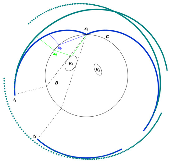
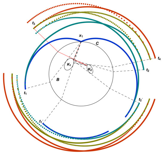
Figure 1 displays the part of $ϵ\left({\mathcal{T}}_{x_1}\right)$ corresponding to travelling-time data for 0 or 1 reflections by $n=2$ obstacles, with $x_1=(0.4,4)$ and C the circle of radius 4 and centre $(0.4,0)$. For $x_0$ starting at $x_1$ and moving south-westerly along C, the blue line from $x_0$ to $x_1$ doesn’t intersect $\partial K$ at all; namely, it is a linear geodesic whose travelling-time data are in ${\mathcal{T}}_0^0\cap {\mathcal{T}}_{x_1}$. As $x_0$ moves downwards towards the endpoint of the dashed tangent, the echograph (shown outside B) traces out a blue curve from $x_1$ to the endpoint $t_1$. The other blue parts of the echograph also correspond to travelling-time data from linear geodesics (0 reflections). The green parts of the echograph in Figure 1 correspond to travelling-time data of geodesics for 1 reflection, such as the green geodesic starting north-westerly from $x_0$ reflecting once on $\partial K_1$ to $x_1$.

Figure 1. Part of the echograph (0 and 1 reflections), in Example 1.

More of the echograph is shown in Figure 2, where parts corresponding to travelling-time data for 2 reflections (olive) and 3 reflections (red) are also incorporated. For instance, the twice-reflecting red geodesic tangent to $\partial K_1$ defines the cusp $t_3$ on the echograph. The other cusps also correspond to tangent geodesics, as indicated. The echograph is mainly smooth, but different smooth arcs (blue, green, olive and red) meet in cusps, and 6 transversal self-intersections are seen. The smooth arcs in Figure 2 are some of the $ϵ\left({\alpha }_i\right)$ where the ${\alpha }_i$ are the open intervals of Proposition 3 (in no particular order). Cusps (labelled $t_1,t_1^{\prime },t_2,t_2^{\prime },t_3,t_4$) correspond to tangencies of geodesics ending at $x_1$ to $K_1$ or $K_2$.

Figure 2. More of the echograph in Example 1.

Our construction of K uses each cusp in an echograph to determine a pair of lines, one of which is tangent to $\partial K$. By Lemma 1, there is a tangent line which is the extension of either the initial segment of the geodesic from $x_0$, or the terminal segment to $x_1$. The pair of lines is determined from $\mathcal{T}$ using the echograph (additional work is carried out later to determine which of these is tangent). Then 1-parameter families of tangent lines are constructed by varying the echograph which depends on $x_1\in C$. Finally, the $\partial K_i$ are found as unions of envelopes of families of tangents.

Next we augment ${\mathcal{T}}_{x_1}$ and $\mathcal{T}$ to data sets ${\tilde{\mathcal{T}}}_{x_1}$ and $\tilde{\mathcal{T}}$ that include the initial velocities of geodesics. We first exclude points of intersection of the open arcs ${\alpha }_i={\alpha }_{i,x_1}$ in Proposition 3 (these points are reinserted later) by defining ${\alpha }_i^{*}={\alpha }_{i,x_1}^{*}:={\alpha }_i-{\cup }_{i^{\prime }\ne i}{\alpha }_{i^{\prime }}$.

Remark 1.

Any ${\alpha }_i$ intersects at most finitely many ${\alpha }_{i^{\prime }}$. Because intersections of ${\alpha }_i$ and ${\alpha }_{i^{\prime }}$ are transversal for $i\ne i^{\prime }$, ${\mathcal{T}}_{x_1}^{0*}:={\cup }_{i\in I}{\alpha }_{i,x_1}^{*}$ is dense in ${\mathcal{T}}_{x_1}^0:={\cup }_{i\in I}{\alpha }_{i,x_1}$, and

$${\mathcal{T}}^{0*}:=\{(x_0,x_1,t):(x_0,t)\in {\mathcal{T}}_{x_1}^{0^{*}},x_1\in C\}\mathit{is}\mathit{dense}\mathit{in}$$

$${\mathcal{T}}^0:=\{(x_0,x_1,t):(x_0,t)\in {\mathcal{T}}_{x_1}^0,x_1\in C\}.$$

Remark 2.

The ${\alpha }_{i,x_1}^{*}$ partition ${\mathcal{T}}_{x_1}^{0*}$. The generators ${\varphi }_i$ restrict to $C^{\infty }$ functions on the open subsets

$$D_{i,x_1}:=\{c\in C:(c,t)\in {\alpha }_{i,x_1}^{*}\}$$

of C.

For $(x_0,t)\in {\mathcal{T}}_{x_1}^{0*}$, define $u_0=u_{x_0,t,x_1}$ to be the unit vector $-\nabla {\varphi }_i\left(x_0\right)$ pointing inwards from C. Then set

$${\tilde{\mathcal{T}}}_{x_1}^{0*}:=\{(x_0,u_0,t):(x_0,t)\in {\mathcal{T}}_{x_1}^{0*}\}\mathrm{and}{\tilde{\mathcal{T}}}^{0*}:=\{(x_0,u_0,x_1,t):(x_0,u_0,t)\in {\tilde{\mathcal{T}}}_{x_1}^{0*}\}.$$

To reinsert the excluded points, define ${\tilde{\mathcal{T}}}^0$ to be the closure of ${\tilde{\mathcal{T}}}^{0*}$ in

$${\displaystyle \{(x_0,u_0,x_1,t):(x_0,x_1,t)\in {\mathcal{T}}^0\mathrm{with}{u}_0\in S^1\},}$$

and ${\tilde{\mathcal{T}}}_{x_1}^0:=\{(x_0,u_0,t):(x_0,u_0,,x_1,t)\in {\tilde{\mathcal{T}}}^0\}$. Define $\tilde{\mathcal{T}}$ to be the closure of ${\tilde{\mathcal{T}}}^0$ in

$$\{(x_0,u_0,x_1,t):(x_0,x_1,t)\in \mathcal{T}\mathrm{with}{u}_0\in S^1\},$$

and ${\tilde{\mathcal{T}}}_{x_1}:=\{(x_0,u_0,t):(x_0,u_0,x_1,t)\in \tilde{\mathcal{T}}\}$. For $q\ge 1$ define

$${\tilde{\mathcal{T}}}^q:=\{(x_0,u_0,x_1,t)\in \tilde{\mathcal{T}}:(x_0,x_1,t)\in {\mathcal{T}}^q\}.$$

5. Singly-Tangent Geodesics

Summarising so far, for $x_1\in C$:

• ${\mathcal{T}}_{x_1}$ is read directly from $\mathcal{T}$;
• ${\mathcal{T}}_{x_1}^{+}:={\mathcal{T}}_{x_1}^1\cup {\mathcal{T}}_{x_1}^2$ (respectively ${\mathcal{T}}_{x_1}^0$) is the non-smooth (respectively smooth) part of ${\mathcal{T}}_{x_1}$;
• we have seen how to find arcs ${\alpha }_{i,x_1}$ and generators ${\varphi }_i$ for ${\mathcal{T}}_{x_1}^0$;
• ${\tilde{\mathcal{T}}}_{x_1}^{+}:={\tilde{\mathcal{T}}}_{x_1}^1\cup {\tilde{\mathcal{T}}}_{x_1}^2$ and ${\tilde{\mathcal{T}}}_{x_1}^0$ are obtained using the ${\varphi }_i$;
• ${\tilde{\mathcal{T}}}^{+}:={\tilde{\mathcal{T}}}^1\cup {\tilde{\mathcal{T}}}^2$ and ${\tilde{\mathcal{T}}}^0$ are found by varying $x_1$.

Proposition 5, below, is a structural result, analogous to Proposition 3, which will be used to distinguish ${\tilde{\mathcal{T}}}^1$ from ${\tilde{\mathcal{T}}}^2$. A geodesic ${\gamma }^{*}\in \mathrm{\Gamma }$ is said to be bitangent when it has two points of tangency to $\partial K$. Recall that ${\gamma }^{*}$ is linear when it has no other points of contact with $\partial K$.

Proposition 5.

For a countable locally finite family $\tilde{\mathcal{B}}=\{{\tilde{\beta }}_j:j\ge 1\}$ of disjoint bounded open $C^{\infty }$ arcs in ${\tilde{\mathcal{T}}}^{+}$:

1.

${\tilde{\mathcal{T}}}^1={\cup }_{j\ge }{\tilde{\beta }}_j$;

2.

for $1\le j\le 4(n^2-n)$; ${\tilde{\beta }}_j=\{(x_0,(x_1-x_0)/t,x_1,t):(x_0,x_1,t)\in {\beta }_j\}$, where the ${\beta }_j$ are the vacuous arcs in ${\mathcal{T}}_0^1$, defined in Section 2;

3.

for every $j\ge 1$ (Including possibly $j>4(n^2-n)$) there is a diffeomorphism ${\psi }_j:V_j\to {\tilde{\beta }}_j$ where $V_j$ is an open arc in C, and ${\psi }_j\left(x_0\right)\in \left\{x_0\right\}\times S^1\times C\times (0,\infty )$ for all $x_0\in V_j$;

4.

each $(x_0^{*},u_0^{*},x_1^{*},t^{*})\in {\tilde{\mathcal{T}}}^2$ is an endpoint of four open arcs ${\tilde{\beta }}_j,{\tilde{\beta }}_{j^{\prime }},{\tilde{\beta }}_{j^{\prime \prime }},{\tilde{\beta }}_{j^{\prime \prime \prime }}$, where three of $V_j,V_{j^{\prime }},V_{j^{\prime \prime }},V_{j^{\prime \prime \prime }}$ are on one side of $x_0^{*}\in C$, and one is on the other side;

5.

${\tilde{\mathcal{T}}}^2={\cup }_{j\ge 1}\partial {\tilde{\beta }}_j$.

Proof. 

For $(x_0,u_0,x_1,t)\in {\tilde{\mathcal{T}}}^1$, we have ${\gamma }_{x_0,t{u}_0}\in {\mathrm{\Gamma }}^1$ and ${\gamma }_{x_0,t{u}_0}\left(1\right)=x_1$. Now, ${\gamma }_{x_0,t{u}_0}$ is tangent to $\partial K$ at precisely one point. By Lemma 1, this is either the first or last point of contact with $\partial K$.

If the tangency is first, then perturbing the point of tangency in $\partial K$ gives a small open $C^{\infty }$ arc around $(x_0,t{u}_0,x_1,t)$ contained in ${\tilde{\mathcal{T}}}^1$. Similarly, if the tangency is last, an open $C^{\infty }$ arc in ${\tilde{\mathcal{T}}}^{+}$ is given by perturbing the point of tangency in $\partial K$. Therefore, the path components ${\tilde{\beta }}_j$ of ${\tilde{\mathcal{T}}}^1$ in ${\tilde{\mathcal{T}}}^{+}$ are connected smooth 1-dimensional submanifolds of $C\times S^1\times C\times R$. They are bounded, nonclosed and, for $1\le j\le 4(n^2-n)$, can be listed as augmentations of the ${\beta }_j$. Thus, 1. and 2. hold.

For $(x_0^{*},u_0^{*},x_1^{*},t^{*})\in {\tilde{\mathcal{T}}}^2$, the geodesic ${\gamma }^{*}=x_{x_0^{*},t^{*}{u}_0^{*}}$ is tangent to $\partial K$ at both the first and last points of contact, and nowhere else. Nearby geodesics in ${\mathrm{\Gamma }}^1$ are obtained by maintaining tangency either at a variable first point of contact, or at a variable last point of contact with $\partial K$. The tangencies at first (respectively last) points of contact generate arcs ${\tilde{\beta }}_j,{\tilde{\beta }}_{j^{\prime }}$ (respectively ${\tilde{\beta }}_{j^{″}},{\tilde{\beta }}_{j^{‴}}$) in ${\tilde{\mathcal{T}}}^1$, separated by $(x_0^{*},u_0^{*},x_1^{*},t^{*})$.

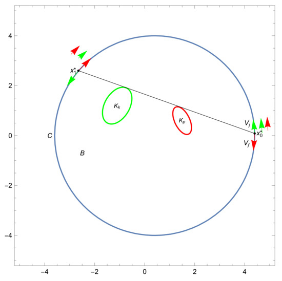
When the bitangent geodesic ${\gamma }^{*}$ is linear, there is an open arc $V_j\subset C$ of initial points of perturbations initially tangent to $\partial K_k$, and another open arc $V_{j^{\prime }}\subset C$ of initial points of perturbations initially tangent to $\partial K_p$, as in Figure 3, where $x_0^{*},V_j,V_{j^{\prime }}$ appear on the right of the illustration. Perturbations whose initial points are in $V_j$ (green) and $V_{j^{\prime }}$ (red) have no other points of contact with $\partial K$. There are also two unlabelled open arcs $V_{j^{″}},V_{j^{‴}}\subset C$ bordered by $x_0^{*}$, consisting of initial points of geodesics whose first points of contact are nontangent to $\partial K$, and whose second points of contact are tangent to $\partial K_k$ (green) or $\partial K_p$ (red), respectively. Similarly, the green and red arrows on the left of Figure 3 and Figure 4 indicate intervals of terminal points of perturbations.

Figure 3. A linear bitangent (proof of Proposition 5).

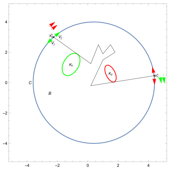
Figure 4. A nonlinear bitangent geodesic (proof of Proposition 5).

Evidently, $j\ne j^{\prime }$, because $V_j$ and $V_{j^{\prime }}$ are on opposite sides of $x_0^{*}$, and similarly, $j^{\prime }\ne j^{\prime \prime },j^{\prime \prime \prime }$ in Figure 3. Indeed, from the geometry of perturbations of $x^{*}$, all of $j,j^{\prime },j^{\prime \prime },j^{\prime \prime \prime }$ are distinct.

In Figure 4, the nonlinear bitangent geodesic ${\gamma }^{*}$ is tangent to $\partial K_k$ and $\partial K_p$ at the first and last points of contact, respectively. It is not tangent anywhere else to $\partial K$, but is reflected at other points of contact, as suggested by the illustration. As before, the nonlinear bitangent is perturbed while maintaining tangency either with $\partial K_k$ (green) or with $\partial K_p$ (red), but now the first and last points of contact remain on $\partial K_k$ and $\partial K_p$, respectively. The initial points of perturbations tangent to $\partial K_k$ sweep out open arcs $V_j,V_{j^{\prime }}\subset C$ (green) on either side of $x_0^{*}$. Initial points of perturbations tangent to $\partial K_p$ give the other intervals $V_{j^{″}},V_{j^{‴}}$ on one side of $x_0^{*}$, as indicated by the two red arrows on the left of Figure 4. Again, $j,j^{\prime },j^{\prime \prime },j^{\prime \prime \prime }$ are distinct.

An element $(x_0,u_0,x_1,t)$ of ${\tilde{\beta }}_j$ corresponds precisely to the point of tangency (first or last contact) of ${\gamma }_{x_0,t{u}_0}$ with $\partial K$. Because there is only one point of tangency it corresponds diffeomorphically to $x_0$. This proves 3.

Thus, that $(x_0^{*},u_0^{*},x_1^{*},t^{*})$ is an endpoint of precisely 4 open arcs and 4. are proved.

Because ${\tilde{\mathcal{T}}}^1$ is open in ${\tilde{\mathcal{T}}}^{+}$, ${\cup }_{j\ge 1}\partial {\tilde{\beta }}_j=\partial {\tilde{\mathcal{T}}}^1\subseteq {\tilde{\mathcal{T}}}^2$. Because ${\tilde{\mathcal{T}}}^1$ is dense in ${\tilde{\mathcal{T}}}^{+}$, ${\tilde{\mathcal{T}}}^2={\cup }_{j\ge 1}\partial {\tilde{\beta }}_j$, proving 5. □

Corollary 2.

${\tilde{\mathcal{T}}}^1$ is the smooth part of the 1-dimensional space ${\tilde{\mathcal{T}}}^{+}$.

Remark 3.

For $j\ge 1$ the $o\left({\gamma }_{x_0,t{u}_0}\right)$ for $(x_0,u_0,x_1,t)\in {\tilde{\beta }}_j$ depend only on ${\tilde{\beta }}_j$. Therefore, we may write them as $o\left({\tilde{\beta }}_j\right)$.

We need the following definitions:

• The open arcs ${\tilde{\beta }}_j\in \tilde{\mathcal{B}}$ where $1\le j\le 4(n^2-n)$ are said to be vacuous;
• For $(x_0,u_0)\in E^2\times S^1$ denote the undirected line through $x_0$ parallel to $u_0$ by $\lambda (x_0,u_0)$;
• For $j\ge 1$ define ${\lambda }_j:V_j\to \mathbb{R}{P}^2$ by ${\lambda }_j\left(x_0\right)=\lambda (x_0,u_0)$ where ${\psi }_j\left(x_0\right)=(x_0,u_0,x_1,t)$;
• Denote the envelope of ${\lambda }_j$ by ${\mathrm{\Lambda }}_{{\tilde{\beta }}_j}:V_j\to E^2$.

6. Extendible Arcs and the Inductive Step

At the end of Section 2 the travelling-time data $\mathcal{T}$ are used to find $4(n^2-n)$ open arcs ${\beta }_j\subset {\mathcal{T}}_0^1$. Each of these is augmented, as described in Proposition 5, to a vacuous open arc ${\tilde{\beta }}_j\subset {\tilde{\mathcal{T}}}^1$. From the definition in Section 2 of the conjugate $\overline{j}$ of j, for $1\le j\le 4(n^2-n)$,

$${\mathrm{\Lambda }}_{{\tilde{\beta }}_j}\left(V_j\right)={\mathrm{\Lambda }}_{{\tilde{\beta }}_{\overline{j}}}\left(V_{\overline{j}}\right).$$

(3)

We also obtain $C^{\infty }$ parameterisations ${\psi }_j:V_j\to {\tilde{\beta }}_j$. More generally (inductively), suppose we have this kind of information where possibly $j>4(n^2-n)$.

In precise terms, suppose we are given a $C^{\infty }$ parameterisation ${\psi }_j:V_j\to {\tilde{\beta }}_j$ of some possibly nonvacuous arc ${\tilde{\beta }}_j\in \tilde{\mathcal{B}}$. Here, $V_j\subset C$ is a maximal open arc with the property that, for all $x_0\in V_j$ and $(x_0,u_0,x_1,t):={\psi }_j\left(x_0\right)$, the first segment of the geodesic ${\gamma }_{x_0,t{u}_0}$ is tangent to $\partial K_k$. The inductive step extends the open arc ${\mathrm{\Lambda }}_{{\tilde{\beta }}_j}\left(V_j\right)\subset \partial K$ by adjoining another such arc to its clockwise endpoint, as follows.

For $x_0^{*}\in C$, the clockwise terminal limit of $x_0\in V_j$, set

$$(x_0^{*},u_0^{*},x_1^{*},t^{*}):=\underset{x_0\to x_0^{*}}{lim}{\psi }_j\left(x_0\right)\in {\tilde{\mathcal{T}}}^2.$$

By Proposition 5, there are three other open arcs ${\tilde{\beta }}_{j^{\prime }},{\tilde{\beta }}_{j^{\prime \prime }},{\tilde{\beta }}_{j^{\prime \prime }}\in \tilde{\mathcal{B}}$ adjacent to ${\tilde{\beta }}_j\subset {\tilde{\mathcal{T}}}^1$ at $(x_0^{*},u_0^{*},x_1^{*},t^{*})$, and the unordered set ${\tilde{\mathcal{B}}}_j:=\{{\tilde{\beta }}_{j^{\prime }},{\tilde{\beta }}_{j^{″}},{\tilde{\beta }}_{j^{‴}}\}\subset \tilde{\mathcal{B}}$ is found by inspecting ${\tilde{\mathcal{T}}}^{+}$. In the proof of Proposition 5, the arcs ${\tilde{\beta }}_j,{\tilde{\beta }}_{j^{\prime }}$ (respectively ${\tilde{\beta }}_{j^{\prime \prime }},{\tilde{\beta }}_{j^{\prime \prime \prime }}$) are generated by geodesics whose first (respectively last) segments are tangent to $\partial K$. From the proof of Proposition 5, ${\tilde{\mathcal{B}}}_j^{*}$ has size 1 or 3. Construct

$${\tilde{\mathcal{B}}}_j^{*}:=\{\tilde{\beta }\in {\tilde{\mathcal{B}}}_j:V\cap V_j=\varnothing \}$$

where $V:=\{x_0:(x_0,u_0,x_1,t)\in \tilde{\beta }\}$.

Definition 2.

$\tilde{\beta }\in {\tilde{\mathcal{B}}}_j^{*}$ is an extension of ${\tilde{\beta }}_j$ when the closure ${\mathrm{\Lambda }}_{j,\tilde{\beta }}$ of ${\mathrm{\Lambda }}_{{\tilde{\beta }}_j}\left(V_j\right)\cup {\mathrm{\Lambda }}_{\tilde{\beta }}\left(V\right)$ is a $C^{\infty }$ strictly convex arc in $E^2$. When an extension of ${\tilde{\beta }}_j$ exists, the arc ${\tilde{\beta }}_j$ is said to be extendible (otherwise nonextendible).

Proposition 6.

If ${\tilde{\beta }}_j$ is extendible, the extension $\tilde{\beta }\in {\tilde{\mathcal{B}}}_j^{*}$ is unique, and ${\mathrm{\Lambda }}_{\tilde{\beta }}\left(V\right)$ is an arc in $\partial K_k$. If ${\tilde{\beta }}_j$ is nonextendible, then ${\tilde{\beta }}_j$ is vacuous and ${\tilde{\beta }}_{\overline{j}}$ is extendible.

Proof. 

By continuity of ${\psi }_j$, the bitangent ${\gamma }_{x_0^{*},t^{*}{u}_0*}$ is tangent to $\partial K_k$ at some $q:=x_{x_0^{*},t^{*}{u}_0*}\left(t_k\right)$ where $0<t_k<1$, and q is a limit of points of first tangency and first contact with $\partial K_k$. By no-eclipse, q is either the first point of contact of the bitangent with $\partial K$ or the second point of contact. □

If q is the first point of contact, then ${\tilde{\beta }}_j$ is extended by ${\tilde{\beta }}_{j^{\prime }}$, whose associated geodesics maintain tangency to $\partial K_k$. Evidently, ${\mathrm{\Lambda }}_{{\tilde{\beta }}_{j^{\prime }}}\left(V_{j^{\prime }}\right)$ is an arc in $\partial K_k$.

For $j^{*}=j^{\prime \prime }$ or $j^{*}=j^{\prime \prime \prime }$, and $({\tilde{x}}_0,{\tilde{u}}_0,{\tilde{x}}_1,\tilde{t})\in {\tilde{\beta }}_{j^{*}}$ near $(x_0^{*},u_0^{*},x_1^{*},t^{*})$, the last points of contact of ${\gamma }_{{\tilde{x}}_0,\tilde{t}{\tilde{u}}_0}$ are tangent to $\partial K$ near $q^{\prime }\in \partial K_{k^{\prime }}$ where $q^{\prime }\ne q$. By the argument in §3 of [1], the $\lambda ({\tilde{x}}_0,{\tilde{u}}_0)$ are not all tangent to a $C^{\infty }$ strictly convex arc; namely, ${\mathrm{\Lambda }}_{{\tilde{\beta }}_{j^{*}}}$ is not strictly convex, and ${\tilde{\beta }}_{j^{*}}$ does not extend ${\tilde{\beta }}_j$. Therefore, the extension $\tilde{\beta }={\tilde{\beta }}_{j^{\prime }}$ is unique.

If, alternatively, q is the second point of contact, then the first point of tangency is at $q^{\prime }:=x_{x_0^{*},t^{*}{u}_0*}\left(s^{\prime }\right)\in \partial K_{k^{\prime }}$ where $0<t_{k^{\prime }}<t_k$ with $k^{\prime }\ne k$. By Lemma 1, $q^{\prime }$ is the first point of contact of the bitangent with $\partial K$. By Lemma 1, and because q is the second point of tangency, the bitangent is linear with $q,q^{\prime }$, the only points of contact with $\partial K$. Therefore, $1\le j\le 4(n^2-n)$, and $q^{\prime }$ is the first point of contact of the linear bitangent ${\gamma }_{x_1^{*},-t^{*}{u}_0^{*}}$ with $\partial K$. Then ${\tilde{\beta }}_{\overline{j}}$ is extended by requiring tangency to $\partial K_k$ of the associated geodesics.

The arc ${\mathrm{\Lambda }}_{{\tilde{\beta }}_j}\left(V_j\right)$ in $\partial K_k$ is therefore extended by an incremental arc ${\mathrm{\Lambda }}_{\tilde{\beta }}\left(V\right)$, where $\tilde{\beta }$ is an extension either of ${\tilde{\beta }}_j$ or of ${\tilde{\beta }}_{\overline{j}}$. This completes the inductive step.

Now the construction of $\partial K$ proceeds as follows. First, ${\tilde{\beta }}_j$ is chosen with $1\le j\le 4(n^2-n)$, and the inductive step is carried out repeatedly with $\tilde{\beta }$ replacing ${\tilde{\beta }}_j$ after each step, until the incremental arcs ${\mathrm{\Lambda }}_{\tilde{\beta }}\left(V\right)$ in $\partial K$ are acceptably small. Countably many repetitions would be needed for perfect reconstruction. Then another vacuous arc is used to restart the iterative process. This is repeated until all the vacuous arcs are used. Finally, $\partial K$ is the union of the closures of all the arcs (initial and incremental) in $\partial K$.

7. Conclusions

For unknown disjoint obstacles $K_1,K_2,\dots ,K_n$ contained in a compact m-manifold manifold with boundary B in Euclidean m-space $E^m$, rays in B from $C:=\partial B$ to itself are reflected in the usual way by $\partial K_1,\partial K_2,\dots ,\partial K_n$ (but not by C). The problem is to find information about the obstacles from measurements of travelling times of reflected rays (geodesics). Even when B and the $K_i$ are smoothly embedded m-dimensional balls, the travelling times sometimes do not determine the obstacles, as seen in the 2-dimensional examples of Livshits and those in [19] where $m>2$. These cases are excluded by requiring B and $K_i$ to be smooth, strictly convex embeddings of the m-dimensional unit ball. Then the $K_i$ are uniquely determined by the travelling times [2] for $m\ge 3$. Unfortunately, the proof in [2] is not constructive and gives no clue about how the $K_i$ might be found. This remains problematic, at least for $n\ge 3$, even when $m=2$.

This most elementary case is studied in the present paper, assuming the no-eclipse hypothesis given in Section 1. Then, the number n of obstacles is found from travelling times using Proposition 1. We go on to reconstruct $K_i$, as follows.

First, Lemma 3 uses travelling-time data of nowhere-tangent geodesics to construct $C^{\infty }$ functions $\varphi :{\mathcal{U}}_0\mapsto (0,\infty )$, from which initial directions of geodesics at points on some subintervals of C can be calculated. Then C is the union of the closures of maximal subintervals. The maximal subintervals are found from the travelling-time functions $\varphi$, using Proposition 3. Corollary 1 identifies endpoints of maximal subintervals by finding cusps in sets ${\mathcal{T}}_{x_1}$ found from travelling times of geodesics that end on points $x_1\in C$. In Section 4, these sets and the cusps are displayed in echographs.

Cusps in echographs correspond to geodesics ending at $x_1$ that are singly tangent to the $\partial K_i$. In Section 5, we keep track of singly tangent geodesics as $x_1$ varies. Proposition 5 finds that the singly tangent geodesics define maximal open intervals in another computable set. The endpoints of the subintervals correspond to geodesics that are twice tangent to $\partial K_i$.

This is all put together in Section 6, where, using no-eclipse, Proposition 6 shows how to find countably many families of lines that are singly tangent to the $\partial K_i$. Then ${\cup }_{i=1}^n\partial K_i$ is determined as the closure of the union of the envelopes of these countably many families. Therefore, in theory, the $K_i$ are completely determined from travelling-times.

This construction is a complicated recipe that would be difficult to implement. In practice, we find only finitely many of the countable families of tangent lines, focusing first on families where lines correspond to geodesics that are once, twice, or maybe three times reflected. Even this requires extremely accurate measurements of travelling times, very large amounts of data and substantial computational effort to detect smooth families of cusps in echographs, then to accurately calculate envelopes. Then, large parts of the $\partial K_i$ are found, but not all. The scope of the present paper is necessarily limited: our ambient space $E^m$ is flat with $m=2$, and the $K_i$ are smooth, strictly convex and satisfy no-eclipse.

References

- Noakes, L.; Stoyanov, L. Lens rigidity in scattering by unions of strictly convex bodies in R2. SIAM J. Math. Anal. 2020, 52, 471–480. [Google Scholar] [CrossRef]
- Noakes, L.; Stoyanov, L. Rigidity of scattering lengths and travelling times for disjoint unions of convex bodies. Proc. Amer. Math. Soc. 2015, 143, 3879–3893. [Google Scholar] [CrossRef]
- Noakes, L.; Stoyanov, L. Traveling times in scattering by obstacles. J. Math. Anal. Appl. 2015, 430, 703–717. [Google Scholar] [CrossRef]
- Stoyanov, L. Santalo’s Formula and stability of trapping sets of positive measure. J. Differ. Equ. 2017, 263, 2991–3008. [Google Scholar] [CrossRef][Green Version]
- Chavel, I. Riemanian Geometry: A Modern Introduction; Cambridge University Press: Cambridge, UK, 1993. [Google Scholar]
- Cornfeld, I.P.; Fomin, S.V.; Sinai, Y.G. Ergodic Theory; Springer: Berlin, Germany, 1982. [Google Scholar]
- Ikawa, M. Decay of solutions of the wave equation in the exterior of several convex bodies. Ann. Inst. Fourier 1988, 38, 113–146. [Google Scholar] [CrossRef]
- Croke, C.; Uhlmann, G.; Lasiecka, I.; Vogelius, M. Geometric Methods in Inverse Problems and PDE Control; Springer Science & Business Media: Berlin, Germany, 2012. [Google Scholar]
- Guillarmou, C. ‘Lens rigidity for manifolds with hyperbolic trapped sets. J. Amer. Math. Soc. 2017, 30, 561–599. [Google Scholar] [CrossRef]
- Guillarmou, C.; Mazzucchelii, M. Marked boundary rigidity for surfaces. Ergodic Th. Dyn. Sys. 2018, 38, 1459–1478. [Google Scholar] [CrossRef]
- Stefanov, P.; Uhlmann, G.; Vasy, A. Boundary rigidity with partial data. J. Amer. Math. Soc. 2016, 29, 299–332. [Google Scholar] [CrossRef]
- Hörmander, L. The Analysis of Linear Partial Differential Operators; Springer: Berlin, Germany, 1985; Volume III. [Google Scholar]
- Melrose, R.; Sjöstrand, J. Singularities in boundary value problems I. Comm. Pure Appl. Math. 1978, 31, 593–617. [Google Scholar] [CrossRef]
- Melrose, R.; Sjöstrand, J. Singularities in boundary value problems II. Comm. Pure Appl. Math. 1982, 35, 129–168. [Google Scholar] [CrossRef]
- Lax, P.; Phillips, R. Scattering Theory; Academic Press: Amsterdam, The Netherlands, 1967. [Google Scholar]
- Lax, P.; Phillips, R. The scattering of sound waves by an obstacle. Comm. Pure Appl. Math. 1977, 30, 195–233. [Google Scholar] [CrossRef]
- Majda, A. A representation formula for the scattering operator and the inverse problem for arbitrary bodies. Comm. Pure Appl. Math. 1977, 30, 165–194. [Google Scholar] [CrossRef]
- Melrose, R. Geometric Scattering Theory; Cambridge University Press: Cambridge, UK, 1995. [Google Scholar]
- Noakes, L.; Stoyanov, L. Obstacles with non-trivial trapping sets in higher dimensions. Arch. Math. 2016, 107, 73–80. [Google Scholar] [CrossRef]
- Plakhov, A. Exterior Billiards: Systems with Impacts Outside Bounded Domains; Springer: New York, NY, USA, 2012. [Google Scholar]
- Plakhov, A.; Roshchina, V. Invisibility in billiards. Nonlinearity 2011, 24, 847–854. [Google Scholar] [CrossRef]
Publisher’s Note: MDPI stays neutral with regard to jurisdictional claims in published maps and institutional affiliations. |
© 2021 by the authors. Licensee MDPI, Basel, Switzerland. This article is an open access article distributed under the terms and conditions of the Creative Commons Attribution (CC BY) license (https://creativecommons.org/licenses/by/4.0/).