Modeling Recoveries of US Leading Banks Based on Publicly Disclosed Data


Wroclaw University of Economics and Business, 53-345 Wroclaw, Poland
Mathematics 2021, 9(2), 188; https://doi.org/10.3390/math9020188
Submission received: 16 December 2020
/
Revised: 4 January 2021
/
Accepted: 13 January 2021
/
Published: 19 January 2021
(This article belongs to the Special Issue Mathematical Methods on Intelligent Decision Support Systems)
Abstract
:The credit risk management process is a critical element that allows financial institutions to withstand economic downturns. Unlike the methods regarding the probability of default, which have been deeply addressed after the financial crisis in 2008, recovery rate models still need further development. As there are no industry standards, leading banks are modeling recovery rates using internal models developed with different assumptions. Therefore, the outcomes are often incomparable and may lead to confusion. The author presents the concept of a unified recovery rate analysis for US banks. He uses data derived from FR Y-9C reports disclosed by the Federal Reserve Bank of Chicago. Based on the historical recoveries and credit portfolio book values, the author examines the distribution function of recoveries. The research refers to a credit card portfolio and covers nine leading US banks. The author leveraged Vasicek’s one-factor model with the asset correlation parameter and implemented it for recovery rate analysis. This experiment revealed that the estimated latent correlation ranges from 0.2% to 1.5% within the examined portfolios. They are large enough to impact the recovery rate volatility and cannot be treated as negligible. It was shown that the presented method could be applied under US Comprehensive Capital Analysis and Review exercise.
1. Introduction
One of the New Basel Capital Accord’s purposes was to reduce the discrepancy between regulatory and economic capital. Therefore, the banking industry is trying to develop and standardize risk management methods. The statistical models recommended by the Basel Committee were supposed to reflect the potential losses more precisely and improve the stability of the banking sector. The Basel Committee is motivating financial institutions to develop their internal risk models. Therefore, they were granted significant autonomy in this area. The banks are expected to conduct their research on credit risk, including portfolio segmentation, parameters estimation, or model validation. The so-called standardized approach is based on Basel I, and is still the most popular method utilized for capital requirement calculation. According to this approach, banks calculate the risk weights dedicated to specific asset classes. These weights reflect the potential unexpected losses. The simple method is now being widely displaced by the IRB approach (Internal Rating Based Approach). According to Basel II [1] the banks are expected to develop internal credit risk models and their further implementation within the risk management process. An additional incentive for banks that decide to implement more advanced methods was a potential capital saving. Some researchers show that advanced techniques may significantly reduce the capital needs regarding credit risk. That especially applies to retail banking. The fifth quantitative research QIS52 clearly showed that some capital benefits are expected for well-diversified retail portfolios.
The approach recommended by the Basel Committee (advanced method) is based on a few elements that impact the credit risk projections. The main factor is the probability of default calculated within the twelve months horizon. The second is the recovery rate (RR), presenting the expected percentage of defaulted exposures which can be recovered due to the debt collection process. Similarly, the LGD parameter (Loss Given Default) is interpreted as an unrecovered part of a loan outstanding and also is expressed as a percentage value. For practical reasons, it is convenient to model RR and then derive LGD. The next element of the comprehensive risk model is EAD (Exposure at Default). EAD represents the value of a credit exposure at the moment of default. The last key element is the borrower asset correlation. Its value significantly affects the unexpected losses, which impacts the capital requirements described in detail by Zeng [2] and Siarka [3].
The banks can choose the approach to risk management and capital requirement calculation. Under the advanced method, they can leverage a foundation or advanced approach (1). By choosing the foundation approach, the banks are obliged to utilize the parameters suggested by the Basel Committee (recovery rate, asset correlation, exposure at default). The advanced approach gives more flexibility by allowing the banks to estimate these risk measures.
In the literature, there are not many publications concerning the problem of LGD calculation. Carey [4] and Frye [5] noticed that recovery rates might depend on the economic cycle. Gupton [6] considered another factor that can affect RR. He noticed that the value of the collateral is strongly correlated with the value of the recovery rate. A cross-sectional analysis of recovery rates was also presented by Franks [7]. He examined corporate loans granted by European banks. Schafer and Koivusalo [8] focused on the relation between the recovery rate and the probability of default. Gieseske [9] also presented some practical solutions regarding the recovery rate.
This paper focuses on the problem of LGD/RR estimation in the banking sector. Several approaches are reviewed in the context of capital requirement calculation. This paper aims to present the results of one-factor model implementation. The outcomes were achieved for retail portfolios of leading US banks. The author is trying to examine the value of correlation resulting from one-factor model applied for credit card portfolios. The positive correlation presence may suggest the existence of a latent market factor (common for all borrowers) that impacts the distribution function of recoveries. As it is presented further, the higher is the correlation, the more volatile are recoveries. It is particularly crucial for credit risk predictions under stress test exercise, as volatile recoveries may cause a significant loss spike. The Basel approach is based on the expected value of recovery rate and volatile PD measure.
On the other hand, the CCAR (Comprehensive Capital Analysis and Review, an annual exercise initiated by the Federal Reserve to assess whether the largest Bank Holdings Companies operating in the United States have sufficient capital to withstand the financial stress) approach requires LGD stressing with adequate macro factors [10]. Therefore, stress testing exercises are performed with regression models. It also needs to be emphasized that recoveries represent post-default events; they last longer and they are usually poorly correlated with macro factors. Therefore, this paper focuses more on RR distribution function. Its shape may let us know the potential changes of recoveries and the probability of its various scenarios.
The paper is organized as follows. The introduction contains the basic definitions of risk parameters used in the banking industry and a literature review. The next part focuses on one-factor model recommended by the Basel Committee. Later, some remarks on calculation DPD (Days Past Due) are made. Then, several methods regarding LGD estimation are presented. The last part of the paper contains the research results achieved for retail portfolios and final conclusions.
2. The One-Factor Model and Capital Requirements
Regardless of the selected approach—foundation or advanced—the banks must utilize Merton’s one-factor model [11]. This approach is recommended by the Basel Committee and allows calculation of the capital cushion preventing the banks from bankruptcy. According to this approach, the default event appears when the borrower assets’ value drops below a specific limit. Below this limit, the company shareholders have not further incentive to continue the business. It is just more rational to announce bankruptcy and stop paying back the loan. According to this theory, the asset value of i-th company is presented by the following equation:
where Y is a market factor common for all borrowers. The coefficient reflects the impact of the market factor and the factor relevant to the particular borrower () on the asset value. The parameters are easy to interpret for corporate loans. In the retail banking the interpretation is not so clear. The asset correlation is not directly observed, and therefore its estimation is not trivial. In retail banking should be interpreted as a value of index characterizing the risk level of i-th borrower [4]. Under this approach the variables and are normally distributed with mean equal to zero and standard deviation equal to one.
The default event is represented by a variable . It takes one if the i-th borrower defaults and zero in the other cases. The conditional probability of default for a given value of market factor Y can be presented as follows:
where PD is the expected value of the unconditional probability of default. When the portfolio incorporates n loans with similar default probability (PD), it is possible to calculate the probability of percentage losses for a given portfolio [12].
Thus, for variable , the probability of incurring loss up to the limit x, can be presented [4] as follows:
The above formula was incorporated into Basel Document [1] for capital requirement calculation. It refers to an unexpected loss that exceeds the expected value of the loss. The banks should recognize the expected loss in the profit and loss statement, whereas the capital should cover the unexpected loss. So formally, the capital requirement K is defined as:
Apart from the probability of default, LGD, and asset correlation, there is a constant value 0.999 relating to the market factor. Therefore, the actual loss may exceed the calculated capital limit no more than every one thousand years.
The utilization of the advanced method requires relevant documentation describing the statistical model. It also needs an extensive analysis of the model’s predictive power and stability. Besides, local supervisors of the financial markets shall periodically challenge the applied models.
3. The Default Event and LGD Determinants
The LGD estimation process is crucial for assessing the quality and efficiency of the debt collection process. Usually, it is based on the analysis of cash flows retrieved after the default event. The following equation presents the relation between LGD and RR coefficient
The typical LGD analysis covers the estimation of the distribution function and the recovery process duration analysis. As the recovery process often takes a few years, it is desirable to use a discount rate for cash flows to calculate its present value.
Multiple factors may impact the recovery rate [13]. So-called external factors reflect the macroeconomic environment and affect the borrowers and lenders. The internal factors correspond to the specific character of the borrower. It may refer to, e.g., the value of the collateral, the type of the collateral, internal policy, business strategy, etc.
The LGD calculation approach can be static or dynamic depending on the underlying assumptions regarding the changes of LGD over time. Under the static approach, the recovery rate remains stable over time. Such an assumption was made within CreditRisk+ model [14]. Its further improvements include the stochastic nature of the recovery rate. A beta distribution function was mostly used for that, as it gives decent flexibility in terms of distribution shape. This approach was also used for such models as CreditMetrics or Credit PortfolioView [15].
The dynamic approach assumes that the recovery rate changes over time and can depend on macroeconomic factors such as unemployment, GDP, inflation, etc.
Among critical factors impacting the level of recovery rate is the structure of borrower liabilities. Gupton [16] observed a strong dependence between the liabilities repayment order and the recovery rate. Another critical factor is the type and collateral value.
The researchers also underline that the legal conditions play a vital role, as they can impact a debt collection process’s duration.
It was also observed that the value of exposure at the moment of default affects further recovery rate. Similarly, the prolonged recovery process may in some cases negatively impacts RR due to applied discounting calculus and rising recovery costs. Another critical factor is the time between loan granting and the default event. It was observed that the defaults observed shortly after loan origination come with a low recovery rate. It mainly results from an inadequate risk assessment process, which could misjudge relevant business conditions or could be a fraud result.
To forecast the LGD, it is necessary to specify the beginning and the end of the recovery process. The insolvency event typically determines the start. According to Basel II the default appears when the delay in repayments exceeds 90 days. From this moment, all inflows are being considered as recoveries. This simple definition has a lot of advantages due to its popularity and widespread use. However, it should be emphasized that when the default is recognized much earlier based on, e.g., other qualitative criteria, this modified date of default should be applied.
As DPD (Days Past Due) triggers the default event, it is relevant to define its calculation method. Originally the DPD was calculated as the number of days between the current date and the last date when the overdue balance emerged. Currently, the banks recognize the overdue moment as the oldest maturity date of all overdue installments at the moment of analysis. In other words, the loan installments are treated as a set of “separate” tranches, and therefore the oldest overdue payment indicates the moment of arrear appearance. Moreover, there are more accounting factors to be considered under the DPD calculation process, e.g., overdue interests, overdue penalty interests. or other accrued costs.
4. The Approaches to LGD Calculation
There are three most common approaches towards the recovery rate estimation. The first of them is based on market price analysis of defaulted financial instruments. It refers mainly to bonds and regular loan portfolios. Rating agencies such as Moody’s provide the necessary data required for calculations. Under this approach, it is assumed that the market price reflects a fair value of cash flows incorporating recoveries. So, the market price includes costs of recovery proceedings and other factors affecting the cash flows’ uncertainty embedded in a discount rate.
Another group of methods is strictly linked with cash flows observed during the recovery process. So, the key elements are the repayments time structure and applied discount rate.
Another approach covers a group of methods based on the financial instruments’ spread analysis. According to this method, the surplus of interest rate over the risk-free interest rate reflects financial instrument risk. So, the risk premium incorporates credit risk and further recoveries. As it was presented in the first part of this paper, the expected value of loss depends on PD and LGD. However, it is also worth to mention that the spread incorporates some liquidity premium and other minor risks [17]. This issue was widely discussed by Bakshi, Madan, and Zhang [18].
Gurtler [19] noticed that it is more efficient to calculate the recovery rate when the portfolio is divided into two distinct groups. The first incorporates the loans recognized as write-offs. This group typically contains low-recoverable loans. The second group consists of positively-responded-to-the recovery-process loans. It results from the fact that some receivables are extremely difficult to collect, while the other loans go smoothly through the collection process. The empirical results confirm the efficiency of this approach [20,21].
A two-step model’s structure is based on the coefficient reflecting the probability of being recognized as a write-off. The probability that the loan goes successfully through the recovery process is given as . Based on these two probabilities, the LGD is derived using the following formula:
The LGD is calculated as a weighted sum of two LGDs appropriate for selected groups. The probability can be estimated using the logistic regression model presented by the following formula:
Under this approach, the variables are characteristics of i-th loan/borrower as, e.g. DPD, collateralization rate, borrower income, scoring, grade. It can also refer directly to macroeconomic factors such as GDP, unemployment rate, or inflation.
Belotti and Crook [22] utilized a similar approach. However, the authors focused on LGD estimation using a linear regression model. They excluded all the loans with recovery close to zero and one. Another approach presented by Bellotti was based on the decision tree model. According to this method, two logistic regressions are leveraged (for loans with LGD equal to one and zero). In other cases, when 0 < LGD < 1, the linear regression model was applied. This approach gives satisfactory results when the examined portfolio includes a large number of loans with low and high recovery rates. Under this approach, the LGD is calculated according to the following formula:
where p0i is the probability that LGD is equal to zero for the i-th loan and p1i is the probability that the LGD is equal to one. As it was mentioned before, these probabilities are calculated based on two independently estimated logistic regression models.
Some researchers noticed that also the one-factor model can be leveraged for recoveries estimation. As it was presented earlier, this approach takes into account the systematic risk. Similar to the PD model, the recovery rate may also depend on the market factor. So, under this approach, it is justified to pose a question regarding the range of possible LGD/RR volatility under the adverse market conditions. Dullmann and Trapp [23] presented their results based on the concept developed earlier by Schonbucher [24]. Furthermore, Frye [5] conducted his research focusing on the one-factor method. According to Dullmann the most efficient way is to model recovery rate using logit transformation of a normally distributed random variable . The recovery rate is then presented as:
where:
where X and Wj are normally distributed random variables. The coefficient ω plays a similar role to the asset correlation ρ used under IRB capital requirement model. Its value ranges from zero to one and is constant for all borrowers. The interpretation of variable X and Wj is analogous as earlier. X reflects the systematic risk, while Wj refers to the idiosyncratic risk specific for the j-th borrower. The model utilized by Dullmann and Trapp can be presented in the same way as proposed by Frye [6]:
Frye, however, proposed a more simplified approach using the following model for recovery rate:
The drawback of the above approach is a lack of constraints regarding the recovery rate. Under this method, it can drop below zero and rise above one, which is not be economically justified. However, the simplicity of the model and easy to interpret parameters make this approach sound.
Pykhtin [25], in his survey, leveraged the following model for recovery rate:
According to his approach, the recovery rate was log-normally distributed. This way, he omitted the problem of receiving negative values of RR.
All presented above approaches derived from the one-factor model allow to estimate distribution function for recovery rate. According to the model examined by Dullmann and Trapp, the conditional distribution function is as follows:
For the model proposed by Frye, the density function presents the following formula:
According to the log-normal Pykhtin model, the recovery rate has a distribution function represented by the following formula:
The one-factor model’s implementation requires estimation of coefficient , which is called asset correlation under Basel approach. It was proved by many researchers that default events are correlated [26] due to common market factor. This correlation usually ranges from 1% to 10%, depending on the specific portfolio. Therefore, the correlation among recoveries also needs profound research. It is worth examining whether the recovery rate is sensitive to the market factor. So, the next part of this paper is focused on the following RR model:
where is the expected value of the recovery rate.
According to IFRS 9, the LGD should also include forward-looking macro-economic scenarios, as was presented by Miu and Ozdemir [27]. Joubert et al. [28,29] listed multiple methodologies to model LGD based on the loan-level data. The most popular include the beta regression, inverse beta transformation, survival analysis, and Box–Cox transformation. Siarka [30] applied a Monte Carlo simulation method for portfolio profitability calculation. Under his approach, recoveries were correlated with defaults and interest rates; the method allowed us to calculate financial ratios like return on assets or return on equity. Bijak and Thomas [31] encountered more than 15 different performance measures in the literature concerning LGD models. This clearly reveals the difficulty concerning LGD modeling. The LGD can be modeled using the direct or the indirect approach. Under the direct approach, the LGD is equal to one minus the recovery rate. Under the indirect approach, two components are modeled separately, i.e., the probability component and the loss severity.
5. Empirical Results
The data from FR Y-9C reports were leveraged to examine the impact of the macro factor on the recoveries (https://www.chicagofed.org/webpages/banking/financial_institution_reports/bhc_data.cfm). Currently, all United States Bank Holding Companies are obliged to submit these reports once their consolidated assets exceed 500 million USD. The data is available from 1986 and includes many financial items regarding recoveries, credit risk, and specific portfolios’ volume. For the analysis, the data from Schedule HI-B and HC-C regarding credit cards were leveraged. This portfolio type is a part of loans originated to individuals for household, family, and other personal expenditures.
The FR Y-9C report data are not available at the loan level, so the individual recovery rates cannot be calculated. For further analysis, the ratios of quarterly recoveries (code in FR Y-9C: BHCKB515) in relation to the book value of loans (code in FR Y-9C: BHCKB538) were calculated. It should be emphasized that the measure created this way is not a Basel recovery rate but represents the fraction of recoveries in the total value of the portfolio. However, assuming that the bank’s risk policy is stable over time, and there are no significant changes in the portfolio composition, further conclusions are applicable to typical recovery rates. In other words, the findings regarding the correlation resulting from the one-factor model may be valid, providing that the portfolio outstanding is highly correlated with the value of exposure at default and the recovery process is conducted in the same efficient way over time. These assumptions are quite restrictive; however, they should be met by such standardized portfolios as credit cards in the US.
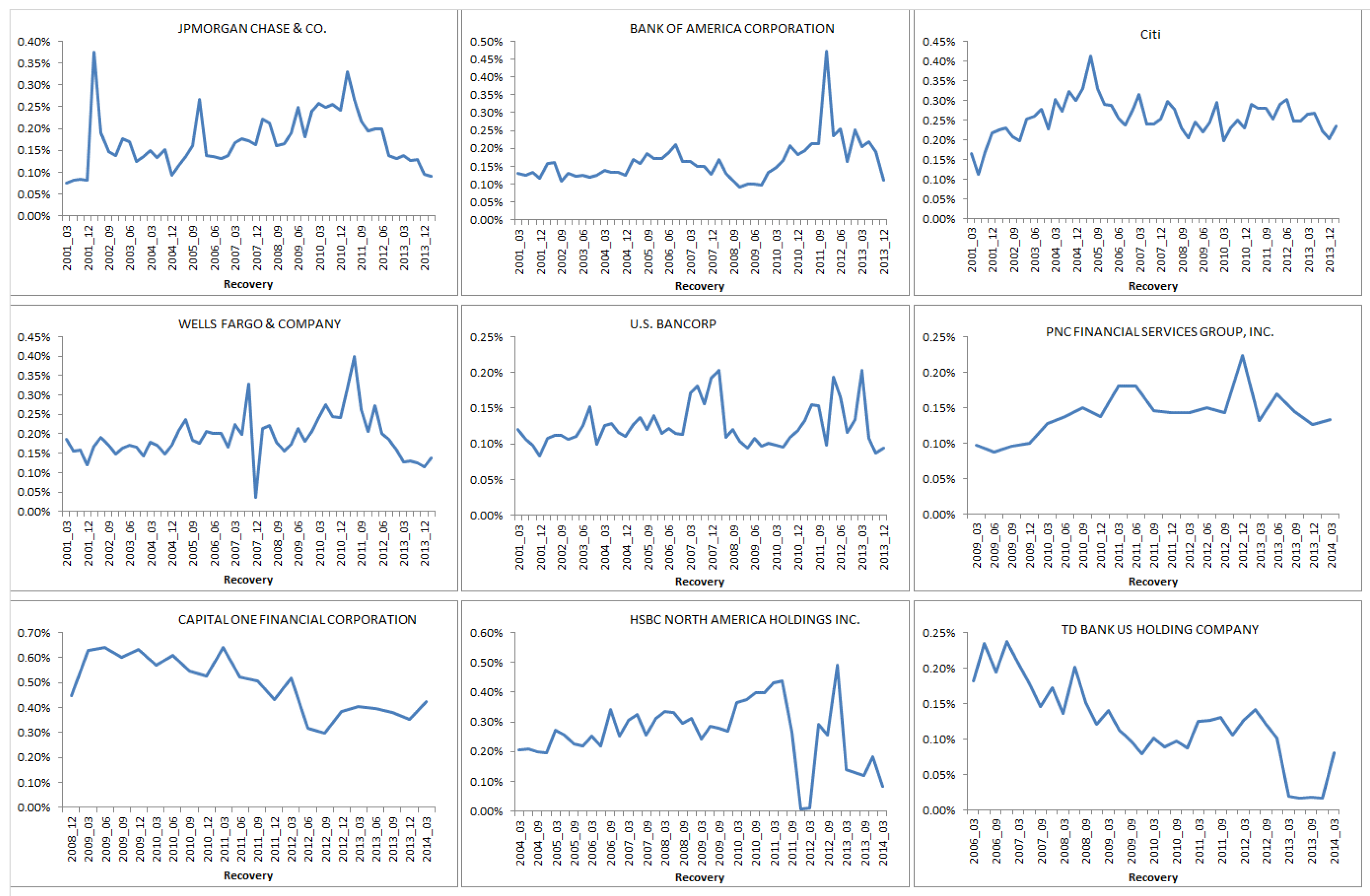
The analysis was performed for nine leading US banks, including JPMorgan Chase & Co., New York, NY, USA, Bank of America Corporation, Citi Group, Wells Fargo & Company, U.S. Bancorp, PNC Financial Services Group inc., Capital One Financial Corporation, HSBC North America Holding Inc. and TD Bank US Holding Company. Figure 1 presents recovery ratios calculated for all selected banks according to the specified procedure. For the first five banks, the data were available from I quarter 2001 up to I quarter 2014. For PNC Financial Services Group Inc. and Capital One Financial Corporation, the data were available from I quarter 2009 and IV quarter 2008, respectively. For TD Bank, the data were available since 2006 and for HSBC from 2004.
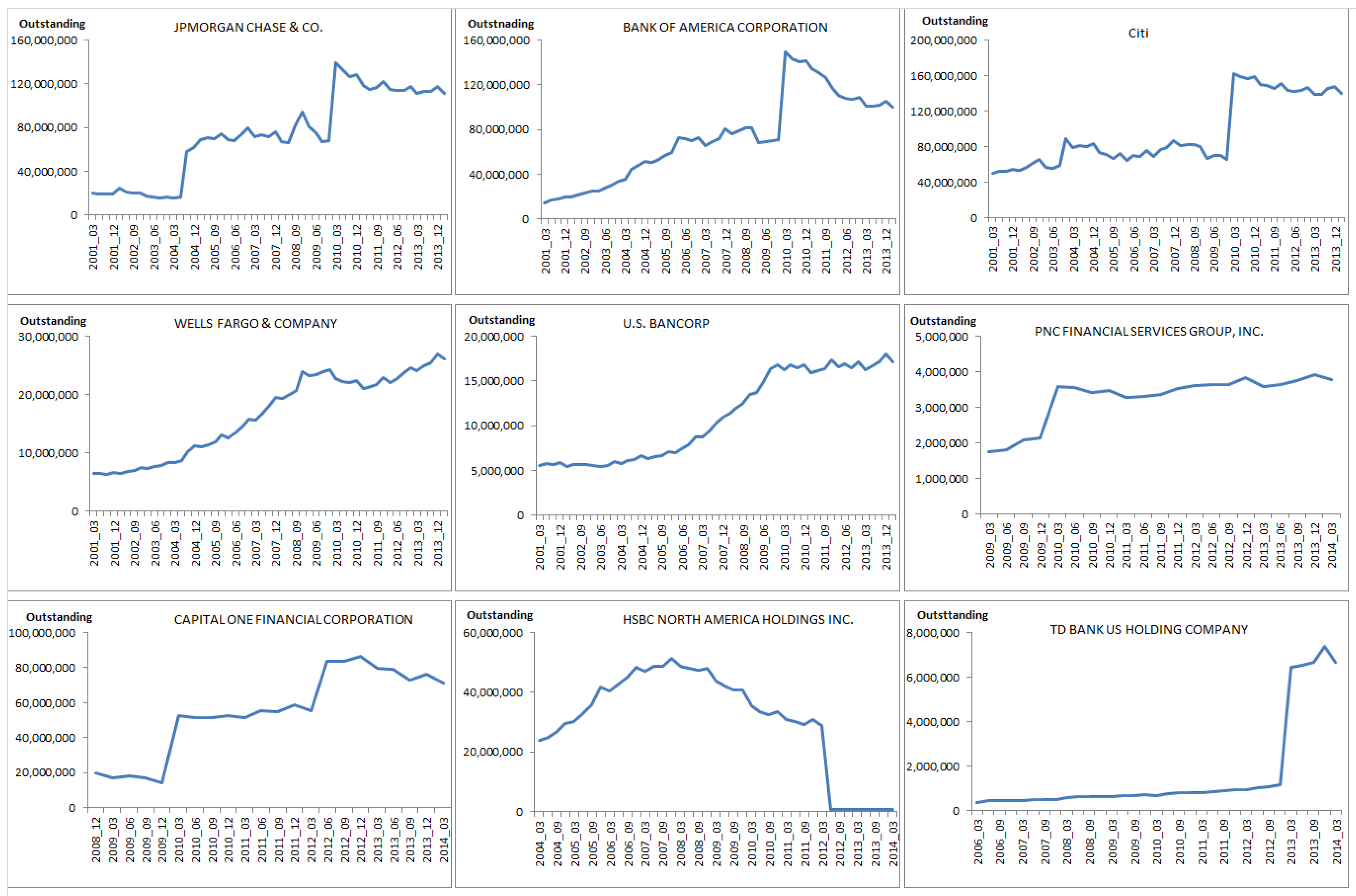
Figure 2 presents outstanding (credit cards) of particular banks available in FR Y-9C reports. It clearly shows that most banks encountered at least one spike during the last few years. These dynamic changes resulted from mergers, acquisitions, or portfolio sales. However, it shall be noticed that these changes didn’t impact long-run recovery rates significantly, which can be observed in Figure 1.
The spike in JPMorgan Chase outstanding observed in 9/2010 is not observed on the recovery rate chart. Higher recoveries balanced the increase of the outstanding, and this is why recovery rates did not change significantly. However, in some cases, a single spike can be noticed. It results from a delay in the recovery reporting process. It can be observed for Citi Bank, Bank of America, and Capital One Financial Corporation.
An exceptionally massive change of outstanding was observed for HSBC (6/2012) as well as TD Bank (6/2012). At that time, HSBC made a transaction resulting in portfolio shrinking, while TD Bank reported significant growth of its assets. In both cases, these changes impacted the long-run recoveries what is observed in Figure 1.
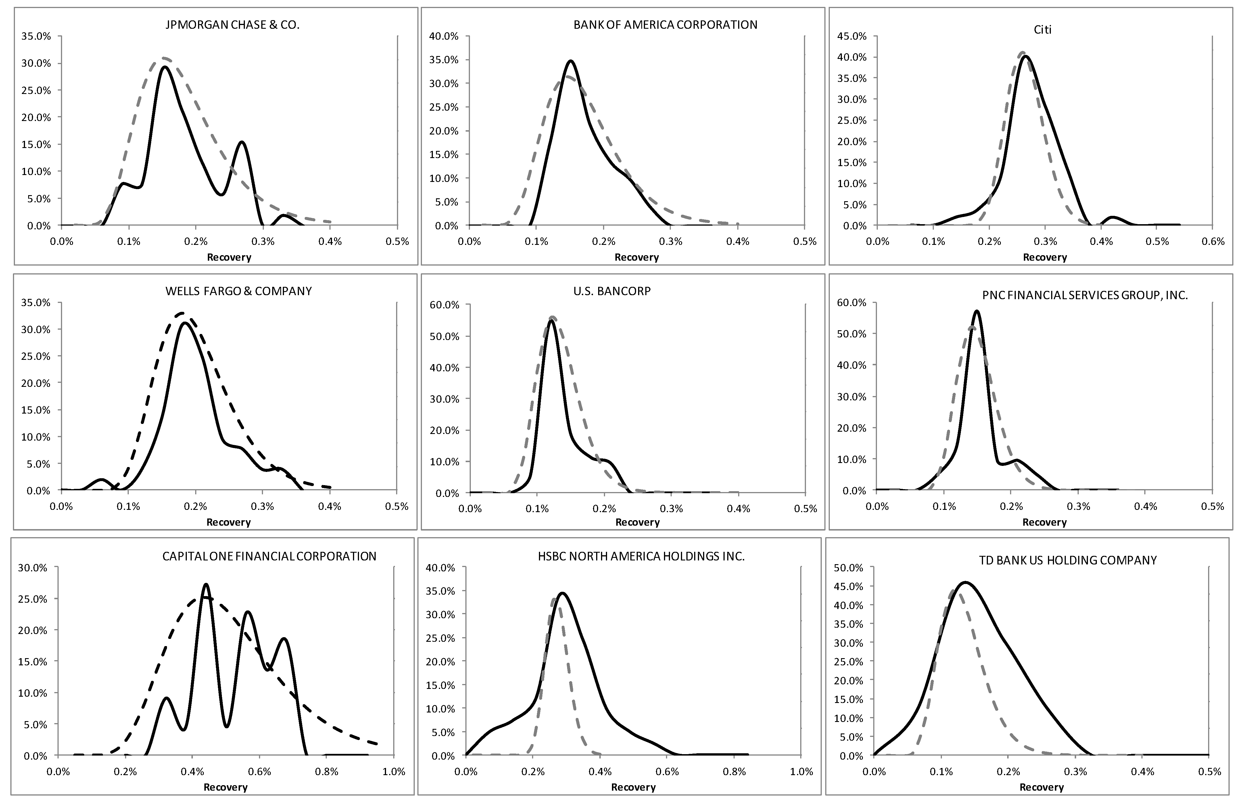
The ratios presented in Figure 1 were used to estimate distribution functions (Figure 3). Table 1 shows basic statistics, including average, standard deviations, and model values. The average values range from 0.12% to 0.49% and concentrate around 0.2%. Standard deviations are not large and range from 0.03% to 0.11%. The highest average value and the highest standard deviation were observed for Capital One Financial Corporation. For this bank, the data is scarce, as it includes only 22 quarters starting from IV quarter 2008. Modal values appeared to be slightly lower than average values, which suggests that the distribution functions are right-skewed.
As was mentioned above, the distribution functions presented in Figure 3 are right-skewed. It was assumed that this is the result of the recoveries correlation embedded in the one-factor model. Therefore, the differences between the expected values and the modal values were used to verify the above thesis. Under the one-factor model, the higher is the expected value in relation to the modal value, the stronger is the impact of the market factor on the recoveries (i.e., higher correlation). Furthermore, higher sensitivity to the market factor causes larger volatility of the recovery rate. Based on quarterly aggregated data, the correlation can be calculated based on the following formula [27]:
where is a modal value and is the expected value.
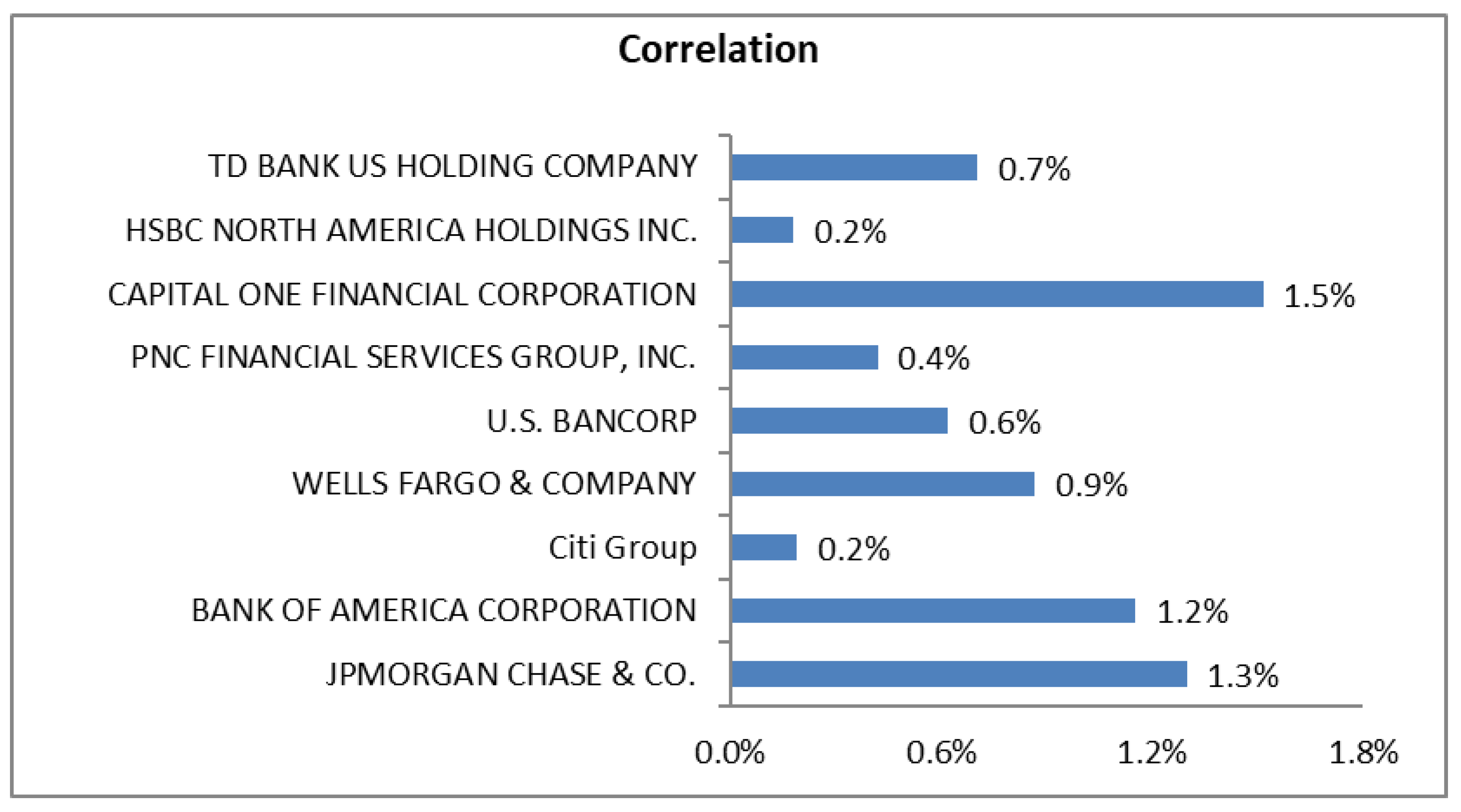
Figure 3 presents the results achieved for selected banks. The correlations appeared to be higher than zero and range from 0.2% to 1.5%. The lowest values (0.2%) were derived for Citi Group and HSBC. The highest value (1.5%) was calculated for Capital One Financial Corporation.
The results are consistent and oscillate at around 1%. So, it can be noticed that the correlation is relatively small. However, it is higher than zero, and therefore, it impacts the shape of distribution functions. It makes it more wide comparing to the zero correlation case.
Figure 4 presents the empirical distribution functions estimated based on historical data (solid lines). For comparison, the theoretical distribution functions were also calculated (dotted lines). The theoretical distributions were calculated based on the one-factor model for given expected values and correlations.
As it can be noticed in Figure 4, the theoretical distribution functions fit quite well the empirical observations. The last row representing the outcomes for Capital One Financial Corporation, HSBC, and TD Bank reveals some discrepancies. However, it shall be emphasized that the time series of these banks were relatively short. Therefore, large estimation errors may explain some inaccuracies. So, in these cases, it is worth recalculating the model again once the time series will cover at least 40 quarters.
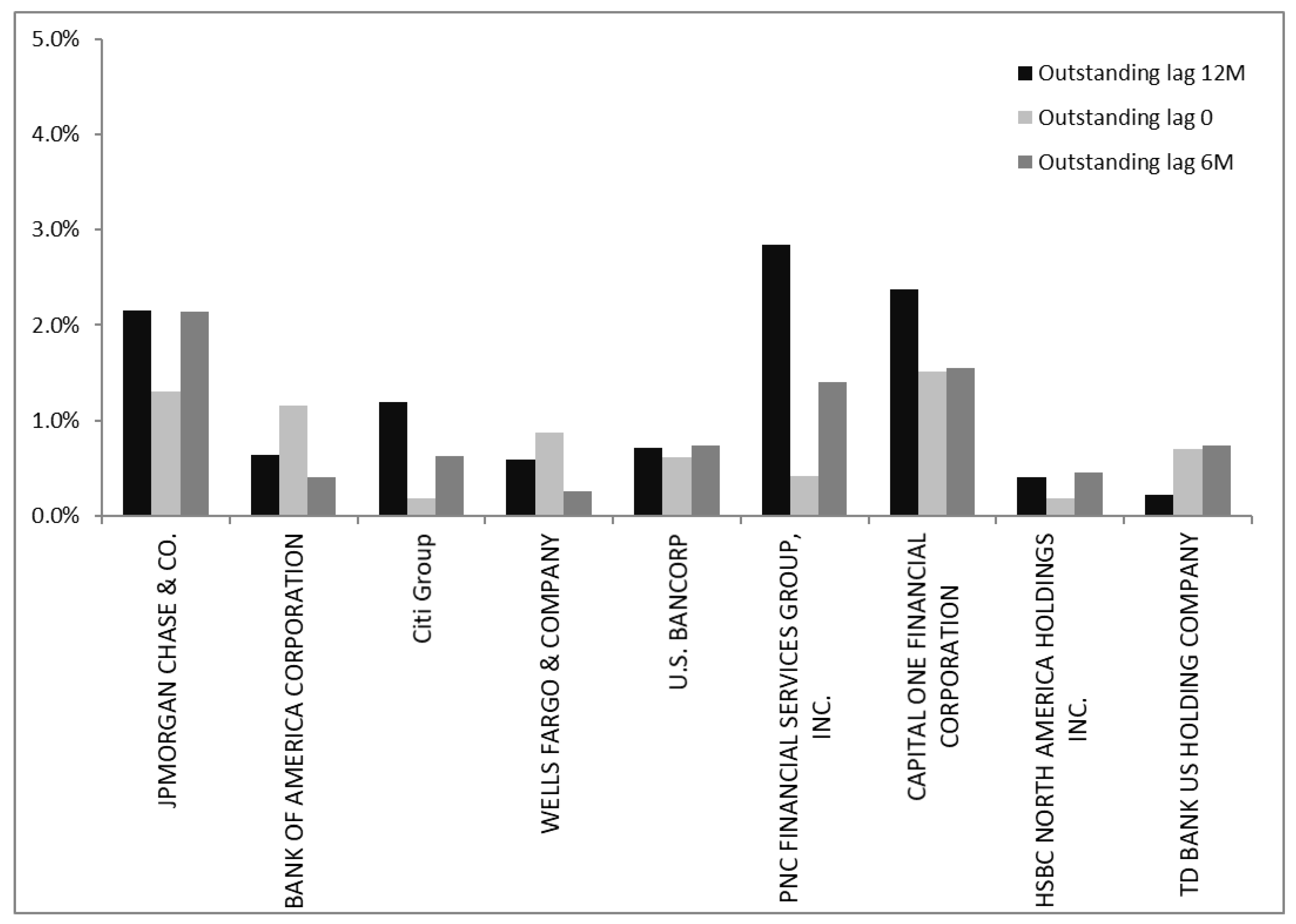
For the validity of the conclusions, the portfolio’s composition should not change substantially over time. Moreover, there should not be serious portfolio acquisitions. Therefore, the correlations were calculated with various lags with respect to outstanding value. It was expected that correlations would not be substantially sensitive to shift in time (lag of the outstanding). The results of this exercise are presented in Figure 5, where zero, two, and four quarters lags were analyzed.
As can be observed, the correlation results are consistent for most of the banks. The most considerable differences were observed for PNC Financial Services, where both 6 M and 12 M lag resulted in higher correlation. Furthermore, Citi Group revealed a substantial change. However, it should be noticed that the overall range of correlation was not changed substantially. The banks with initially calculated low correlations are still below an average. That proves that the proposed method is robust and can be utilized to estimate the correlation and calculate recoveries’ distribution function.
The correlation estimates are at around one percent and show a relatively small impact of a latent macro factor on recoveries. However, these values are large enough to skew the distributions, as is presented in Figure 4.
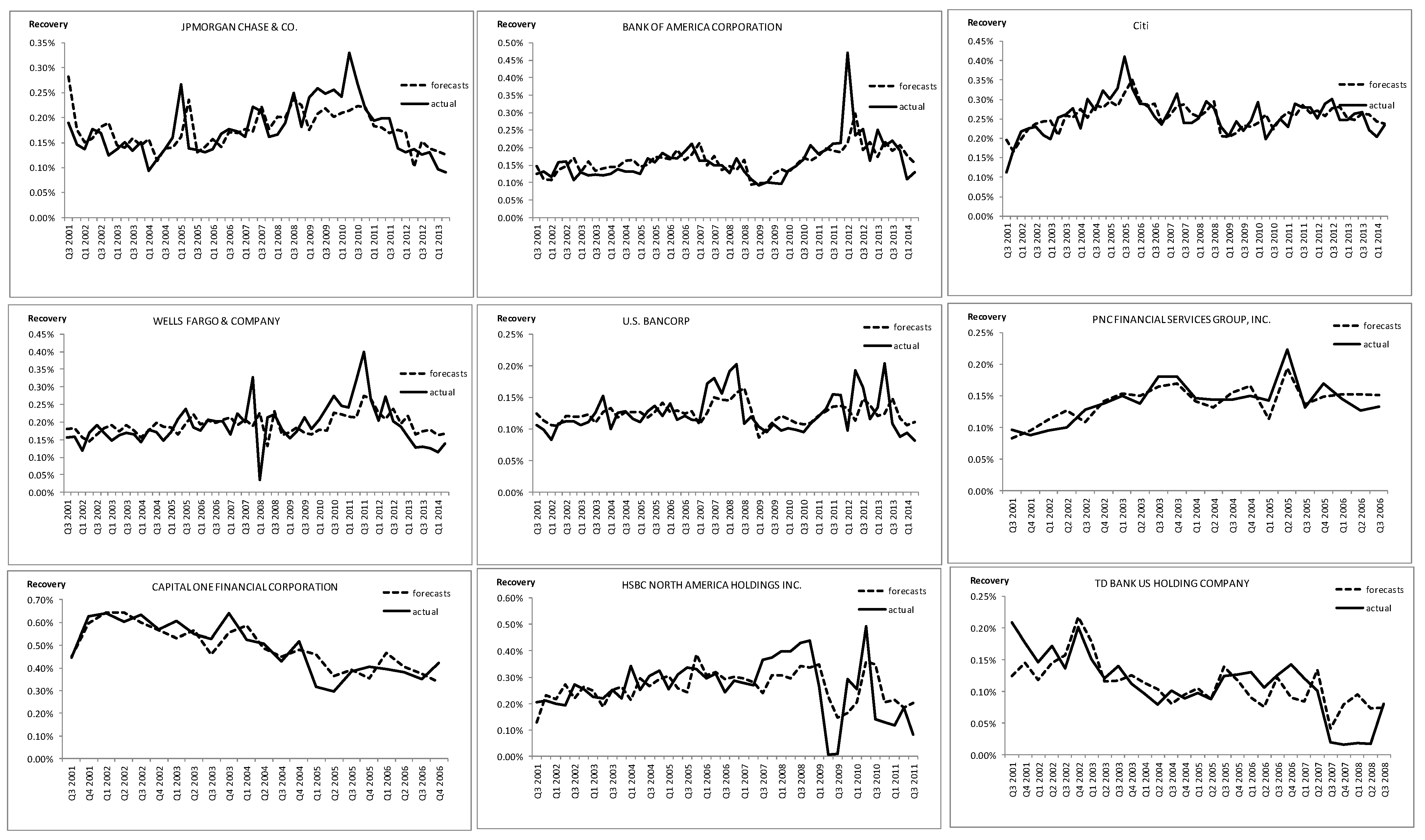
The FED recommends that under the CCAR exercise, the macro factors should be leveraged. Therefore, a complementary analysis was performed, and autoregressive models with external macro factors as regressors were developed. The following candidate variables were selected as macro factors: US real GDP growth rate, US unemployment rate, US real disposable income growth, and US CPI inflation rate. For all these variables, lags from 0 to 2 quarters were considered. Additionally, it was assumed that each variable could enter the model only once, i.e., one variable could not be used with two distinct lags. In order to find the best fitting model for each bank, all possible combinations of macro factors were analyzed. Figure 6 shows the results presenting actual and forecasted values.
Table 2 contains regression outcomes including R-squared, adjusted R-squared and p-values calculated for F statistic. The table’s right panel presents macro factors that appeared to be significant and were selected as regressors. Numbers below the variable names indicate the lag, which was employed for a particular macro factor.
High R-squared values and statistically significant coefficients show that recovery rates could be modeled with macro factors. It was also shown that the one-factor model, based on a latent and common market factor, is adequate for recovery rate projections. Furthermore, the presented approach explains the skewness of the recoveries distribution function by better fitting to the actual data. Therefore, it can be used for recovery projections under severely adverse macroeconomic scenarios.
6. Conclusions
The Basel Committee suggests calculating capital requirements based on PD, EAD, and LGD. These parameters also play a crucial role in AQR (Asset Quality Review) process under the challenger approach for losses estimation. While many researchers widely examine the PD, recovery rates are being poorly explored. In the literature, several attempts are presented towards recovery rate modeling. Some of them are based on the value of collateral, exposure value, or probability of default. In retail banking, where the loans are relatively homogenous and uncollateralized, recovery rates are usually estimated based on expected value. However, the volatility and observed skewness revealed that the recoveries might drop significantly under severely adverse macro scenarios.
The presented research addressed the problem of recovery ratio distribution function estimation. The author used data of nine leading US banks sourced from FR Y-9C reports incorporating information about credit card recoveries. Then, he verified the hypothesis that recoveries in the portfolio are correlated, which impacts the distribution function. It was assumed that the recovery ratio could be modeled under the one-factor approach. Furthermore, it was shown that the analysis could be performed based on publicly disclosed aggregated data, where loan-level data are not available.
The application of the one-factor model for recoveries has profound implications for the banking industry. Under this approach, the recoveries are treated as correlated. Similar to defaults, they are linked with idiosyncratic risk and market factor. Therefore, recoveries shall reveal significantly higher volatility, which is particularly important under stress test projections. Additionally, the distribution functions should be skewed, and consequently, modal values should be lower than expected values.
The research proved that recovery ratios are right-skewed for all selected leading US banks. The correlations oscillate around 1% ranging from 0.2% to 1.5%. It was also shown that it impacts the shape of the distribution function significantly.
The problem of recovery rate projection in the context of the adverse market condition needs further examination. In order to minimize the estimation error, a more extended time series should be utilized. Furthermore, data reflecting recovery rates instead of recovery ratios should be examined. Finally, the presented approach needs to be challenged with loan-level data models, i.e., bottom-up analysis.
Funding
This research received no external funding.
Institutional Review Board Statement
Not applicable.
Informed Consent Statement
Not applicable.
Data Availability Statement
The data presented in this study are openly available in https://www.chicagofed.org/applications/bhc/bhc-home.
Conflicts of Interest
The author declare no conflict of interest.
References
- Basel Committee on Banking Supervision (BCBS). International Convergence on Capital Measurement and Capital Standards; Bank for International Settlements: Basel, Switzerland, 2006. [Google Scholar]
- Zeng, B.; Zhang, J. An Empirical Assessment of Asset Correlation Models; KMV LLC: San Francisco, CA, USA, 2006. [Google Scholar]
- Siarka, P. Asset correlation of retail loans in the context of the new Basel Capital Accord. J. Crédit. Risk 2014, 10, 97–116. [Google Scholar] [CrossRef]
- Carey, M. Credit Risk in Private Debt Portfolios. J. Financ. 1998, 53, 1363–1387. [Google Scholar] [CrossRef]
- Frye, J. Depressing recoveries. Risk 2000, 13, 108–111. [Google Scholar]
- Gupton, G.M. Bank Loan Loss Given Default; Global Credit Research; Moody’s: New York, NY, USA, 2000. [Google Scholar]
- Franks, J.; de Servigny, A.; Davydenko, S. A Comparative Analysis of the Recovery Process and Recovery Rates for Private Companies in the UK, France and Germany; Risk Solutions; Standard & Poor’s: New York, NY, USA, 2004. [Google Scholar]
- Schafer, R.; Koivusalo, A. Dependence of Defaults and Recoveries in Structural Credit Risk Models. 2011, pp. 1–9. Available online: http://arxiv.org/abs/1102.3150 (accessed on 15 August 2020).
- Giesecke, K. Credit Risk Modeling and Valuation: An Introduction. SSRN Electron. J. 2003, 16, 487. [Google Scholar] [CrossRef] [Green Version]
- Siarka, P. CCAR stress tests. Is regression the only tool for losses projection? J. Risk Model Valid. 2015, 9. [Google Scholar]
- Merton, R.C. On the Pricing of Corporate Debt: The Risk Structure of Interest Rates. J. Financ. 1974, 29, 449–470. [Google Scholar]
- Vasicek, O. The distribution of loan portfolio value. Risk 2002, 15, 160–162. [Google Scholar]
- Kozłowksi, Ł. Analysis of the recovery rates in the bank in conditions of limited data availability. Mater. Stud. 2009, 244. [Google Scholar]
- Credit Suisse First Boston. CreditRisk+ a Credit Risk Management Framework. 1997. Available online: http://www.csfb.com/institutional/research/assets/creditrisk.pdf (accessed on 10 January 2015).
- Saunders, A.; Linda, A. Credit Risk Measurement. New Approaches to Value at Risk and Other Paradigms; John Willey & Sons: Hoboken, NJ, USA, 1999. [Google Scholar]
- Gupton, G.M.; Stein, R. A Matter of Perspective. Credit Mag. 2001, 2, 22–23. [Google Scholar]
- Unal, H.; Madan, D.; Guntay, L. Pricing the Risk of Recovery in Default with APRViolations. J. Bank. Finan. 2003, 27, 1001–1025. [Google Scholar] [CrossRef]
- Bakshi, G.; Madan, D.B.; Zhang, F. Recovery in Default Risk Modeling: Theoretical Foundations and Empirical Applications; Division of Research & Statistics and Monetary Affairs, Federal Reserve Board: Washington, DC, USA, 2001. [Google Scholar]
- Gurtler, M.; Hibbeln, M. Pitfalls in Modeling Loss Given Default of Bank Loans. Working Paper. University of Braunschweig. 2011. Available online: https://www.econstor.eu/obitstream/10419/55246/1/684986302.pdf (accessed on 12 October 2020).
- Chen, R.; Wang, Z. Curve Fitting of the Corporate Recovery Rates: The Comparison of Beta Distribution Estimation and Kernel Density Estimation. PLoS ONE 2013, 8, e68238. [Google Scholar] [CrossRef] [PubMed]
- Mora, N. What Determines Creditor Recovery Rates? Fed. Reserve Bank Kans. City Econ. Rev. 2012, 97, 79–109. [Google Scholar]
- Bellotti, T.; Crook, J. Modelling and Predicting Loss Given Default for Credit Cards. Working Paper. Quantitative Financial Risk Management Centre. 2007. Available online: https://www.researchgate.net/publication/215991677_Modelling_and_predicting_loss_given_default_for_credit_cards (accessed on 4 June 2020).
- Dullmann, K.; Trapp, M. Systematic Risk in Recovery Rates—Anempirical Analysis of U.S. Corporate Credit Exposures. Manuscript, Deutsche Bundesbank. 2004. Available online: https://papers.ssrn.com/sol3/papers.cfm?abstract_id=2793954 (accessed on 23 May 2020).
- Schonbucher, P.J. Credit Derivatives Pricing Models: Models, Pricing and Implementation; Wiley: New York, NY, USA, 2003. [Google Scholar]
- Pykhtin, M. Unexpected recovery risk. Risk 2003, 16, 74–78. [Google Scholar]
- Siarka, P. Estimation of Asset Correlation of Retail Exposures Based on Car Loans in Poland. National Bank of Poland. 2011. Available online: https://bankikredyt.nbp.pl/home.aspx?c=%2fascx%2fsearch.ascx (accessed on 14 October 2020).
- Miu, P.; Bogie, O. Adapting the Basel II advanced internal ratings-based models for International Financial Reporting Standard 9. J. Credit Risk 2017, 13, 53–83. [Google Scholar] [CrossRef]
- Joubert, M.; Verster, T.; Raubenheimer, H. Default weighted survival analysis to directly model loss given default. S. Afr. Stat. J. 2018, 52, 173–202. [Google Scholar]
- Joubert, M.; Verster, T.; Raubenheimer, H. Making use of survival analysis to indirectly model loss given default. ORiON 2019, 34, 107–132. [Google Scholar] [CrossRef]
- Siarka, P. Simulation Analysis of Profitability of Retail Loans: Stress Testing, Bank and Credit; National Bank of Poland: Warsaw, Poland, 2012; pp. 81–103. [Google Scholar]
- Bijak, K.; Lyn, C.T. Underperforming performance measures? A review of measures for loss given default models. J. Risk Model Valid. 2018, 12, 1–28. [Google Scholar] [CrossRef]
Figure 1.
Relations of recoveries to the total value of the portfolio. Source: Author’s work.

Figure 2.
Credit card outstanding reported by banks in FR Y-9C [kUSD]. Source: Author’s work.

Figure 3.
The correlations derived for recoveries. Source: Author’s work.

Figure 4.
Distribution functions of recovery ratios (recoveries/portfolio value). Source: Author’s work.
Figure 4.
Distribution functions of recovery ratios (recoveries/portfolio value). Source: Author’s work.

Figure 5.
Correlations calculated for various lags of outstanding. Source: Author’s work.

Figure 6.
Recovery rates—regression forecasts vs. actual values. Source: Author’s work.


Table 1.
Basic statistics for recovery ratios.
| Bank | Average | Std.Dev | Modal |
|---|---|---|---|
| JPMORGAN CHASE & CO. | 0.17% | 0.06% | 0.14% |
| BANK OF AMERICA CORPORATION | 0.16% | 0.06% | 0.14% |
| CITI GROUP | 0.26% | 0.05% | 0.25% |
| WELLS FARGO & COMPANY | 0.19% | 0.06% | 0.17% |
| U.S. BANCORP | 0.12% | 0.03% | 0.11% |
| PNC FINANCIAL SERVICES GROUP, INC. | 0.14% | 0.03% | 0.13% |
| CAPITAL ONE FINANCIAL CORPORATION | 0.49% | 0.11% | 0.41% |
| HSBC NORTH AMERICA HOLDINGS INC. | 0.26% | 0.11% | 0.26% |
| TD BANK US HOLDING COMPANY | 0.12% | 0.06% | 0.11% |
Source: Author’s work.
Table 2.
Regression results.
| Lags [Quarters] | |||||||
|---|---|---|---|---|---|---|---|
| BANK | R-Squared | Adjusted R-Squared | p-Value F Test | Real GDP growth | Real Disposable Income Growth | Unemployment Rate | CPI Inflation Rate |
| JPMORGAN CHASE & CO. | 34.02% | 29.90% | 0.02% | 1 | 2 | ||
| BANK OF AMERICA CORPORATION | 36.40% | 32.42% | 0.01% | 2 | 1 | ||
| Citi | 49.93% | 46.80% | 0.00% | 2 | 0 | ||
| WELLS FARGO & COMPANY | 23.12% | 16.58% | 1.33% | 2 | 1 | 2 | |
| U.S. BANCORP | 24.27% | 21.17% | 0.11% | 1 | |||
| PNC FINANCIAL SERVICES GROUP, INC. | 70.05% | 64.76% | 0.01% | 0 | 2 | 0 | |
| CAPITAL ONE FINANCIAL CORPORATION | 73.52% | 65.25% | 0.03% | 0 | 2 | 0 | 1 |
| HSBC NORTH AMERICA HOLDINGS INC. | 32.57% | 27.10% | 0.20% | 0 | 0 | ||
| TD BANK US HOLDING COMPANY | 50.83% | 44.93% | 0.04% | 1 | 0 | 1 | |
Source: Author’s work.
Publisher’s Note: MDPI stays neutral with regard to jurisdictional claims in published maps and institutional affiliations. |
© 2021 by the author. Licensee MDPI, Basel, Switzerland. This article is an open access article distributed under the terms and conditions of the Creative Commons Attribution (CC BY) license (http://creativecommons.org/licenses/by/4.0/).
Share and Cite
MDPI and ACS Style
Siarka, P. Modeling Recoveries of US Leading Banks Based on Publicly Disclosed Data. Mathematics 2021, 9, 188. https://doi.org/10.3390/math9020188
AMA Style
Siarka P. Modeling Recoveries of US Leading Banks Based on Publicly Disclosed Data. Mathematics. 2021; 9(2):188. https://doi.org/10.3390/math9020188
Chicago/Turabian StyleSiarka, Pawel. 2021. "Modeling Recoveries of US Leading Banks Based on Publicly Disclosed Data" Mathematics 9, no. 2: 188. https://doi.org/10.3390/math9020188
Note that from the first issue of 2016, this journal uses article numbers instead of page numbers. See further details here.