Abstract
Stock index prediction plays an important role in the creation of better investment strategies. However, prediction can be difficult due to the random fluctuation of financial time series. In pursuit of improved stock index prediction, a hybrid prediction model is proposed in this paper, which contains two-step data pretreatment, double prediction models, and smart optimization. In the data pretreatment stage, in order to carry more information about the prediction target, multidimensional explanatory variables are selected by the Granger causality test, and to eliminate data redundancy, feature extraction is inserted with the help of principal component analysis; both of these can provide a higher-quality dataset. Bi-directional long short-term memory and bi-directional gated recurrent unit network, as the concurrent prediction models, can improve not only the precision, but also the robustness of results. In the last stage, the proposed model integrates the weight optimization of the cuckoo search of the two prediction results to take advantage of both. For the model performance test, four main global stock indices are used. The experimental results show that our model performs better than other benchmark models, which indicates the potential of the proposed model for wide application.
1. Introduction
For the past few years, increased globalization, especially in the field of economics, has changed the world enormously. Connections between different countries and regions are becoming closer and closer, which can be seen not only in trading markets of goods and services, but also in capital markets all over the world. The number of global investors is growing fast, as is the scale of investment capital. In other words, due to the rapid development of the global economy, financial investments play an increasingly important role for investors overseas. Therefore, it is of great importance for investors to make precise predictions of stock indices, because the better their prediction, the more they earn. There are also many benefits for policymakers in maintaining market order if stock index prediction can be made more precise [1]. However, based on past studies, precise prediction of stock indices is not easy. The biggest problem is in the random fluctuation of financial time series. The movement of stock indices is influenced not only by fundamental elements, but also by emergency eruption, which creates many difficulties in precise prediction. As a result, many researchers have explored this field, and the search for improved stock index prediction is ongoing [2].
Many prediction models have been developed over the years, which can be categorized into two basic types according to existing studies: traditional statistical methods and emerging machine learning methods.
Traditional statistical methods dominated this field in the past. Some excellent models, such as auto-regressive moving average (ARMA) and generalized autoregressive conditional heteroskedasticity (GARCH), still have powerful influence in the prediction field. For instance, Rounaghi and Zadeh adapted ARMA to forecast stock returns of the S&P 500 and the London Stock Exchange with monthly and yearly time groups [3]. Abounoori et al. tried to predict the volatility of stock exchanges using mean GARCH values [4]. Traditional statistical methods have contributed to financial time series prediction for the past few years. However, due to the growing complexity of financial time series, traditional statistical methods seem inadequate. They usually require high data quality, which creates logistical obstacles.
Nonetheless, the data from real stock markets can be very complex, which makes it hard for traditional statistical analysis to provide good predictions [5,6,7]. Consequently, the need for improved prediction drives the search for a better way to accommodate real situations.
Machine learning methods can handle atypical data structure problems. This data handling capacity profits from the growth of computer algorithms, under which the limitations of data structure hypotheses can be solved. This represents important progress in prediction development, as markets in different locations are becoming more relevant with the growth of globalization. Therefore, in recent years, the use of machine learning methods to achieve prediction is becoming increasingly popular among researchers in the field [8]. For instance, Wu and Duan proved that the Elman neural network could achieve good prediction for the Chinese stock market [9]. Qiu et al. tested the effectiveness of predicting stock returns using artificial neural networks (ANNs) [10]. Liu et al. introduced the convolutional neural network (CNN) to forecast exchange rates [11]. Dutta et al. introduced the gated recurrent unit (GRU) to predict bitcoin prices [12].
With further exploration in the prediction field, the use of hybrid or combined models is becoming a popular research area. The impetus for this is the perceived benefits of the complementarity between different models, which has been the subject of much research. Kristjanpoller and Minutolo found that ANN combined with GARCH could improve the prediction model performance with a 25% reduction in mean average percentage error [13]. Baffour et al. introduced the Glosten–Jagannathan–Runkle (GJR) approach, based on ANN, to forecast currency exchange rate volatility, which reduced prediction error [14]. When it comes to long time series prediction, long short-term memory (LSTM) and gated recurrent unit (GRU) seem to be popular and have attracted attention from many researchers [15]. For instance, Alonso-Monsalve et al. combined CNN and LSTM to predict cryptocurrency exchange rates [16]. Kim and Won introduced LSTM based on GARCH and successfully improved the efficiency of stock price volatility prediction [17]. Patil et al. proved that GRU can work as well as LSTM in different dataset environments [18]. The secret of their popularity can be explained by the special structure of recurrent neural networks (RNNs). Usually, when time series become larger, calculations overcome this obstacle with the use of information from a long time ago, which can have a negative effect on prediction results. The design of RNNs excels in this area, because they have stronger storage ability and can use information from both long- and short-term memory cells; this is the most notable feature of RNNs. LSTM and GRU are variants of RNN that have a more advanced structure. They can avoid gradient explosion or gradient disappearance, which simple RNNs cannot. Based on LSTM and GRU, researchers have added bi-directional information flow to neural networks to make full use of the information; these are known as bi-directional LSTM (BILSTM) and bi-directional GRU (BIGRU). Lu et al. introduced BILSTM combined with CNN and an attention mechanism for stock price prediction [19]. Zhu et al. used BIGRU to predict rubber future time series [20]. Amazingly, BILSTM and BIGRU have also shown promise in detection and prediction of COVID-19 infection [21].
The above studies show the good prediction performance of machine learning methods. However, to make precise predictions, a good model requires good data quality. Having a high-quality standard dataset is important to improve the prediction results. There are two main ways to select explanatory variables. Many researchers have developed explanatory variables from internal movement by decomposing the original data. Cao et al. used complete ensemble empirical mode decomposition (CEEMDAN) to provide variables for financial time series prediction [22]. Yang and Lin introduced empirical mode decomposition (EMD) to forecast exchange rates [23]. Others have selected variables from other markets, which were usually related to external influence on the stock markets. When it comes to related selection, researchers have shown a preference for the Granger causality test. For instance, Veli et al. used this test to find out the relationship of stock prices and economic activity nexus in Organization for Economic Cooperation and Development (OECD) countries [24]. Peng et al. used the Granger causality test to check the relevance of China’s stock market and the international oil market [25]. Chen et al. used this test to find relevant variables for the Taiwan stock index [26]. Another study used the test to determine the relation between crude oil and BRICS (Brazil, Russia, India, China) stock markets [27].
However, bringing relative variables into the prediction system will lead to multidimensional explanatory variables, which usually involves massive amounts of data and cannot avoid data redundancy. This redundancy is not helpful for the prediction calculation part, which not only is more time-consuming, but also leads to worse prediction results. Therefore, feature extraction is needed and the dataset must be reconstructed. According to existing papers, principal component analysis (PCA) has excellent performance on feature extraction. Farzana et al. used the PCA algorithm to successfully rebuild intermedia data [28]. Chen and Hao used PCA to extract features and improve stock trading signals prediction [29]. Adnan et al. introduced the same model into compressive sensing-based data aggregation efficiently [30]. Apart from feature extraction, principal component analysis is also a powerful tool for lossy-data compression [31].
Based on previous studies, this paper proposes a novel prediction model that contains multidimensional explanatory variables, feature extraction, two excellent models, and smart optimization. In order to provide sufficient information, the hybrid model first uses the Granger causality test to filter out potential relative variables, which is intended to lay a good foundation for better prediction. However, when collecting huge amounts of data, insignificant information and data redundancy cannot be avoided. Therefore, in the second stage, the hybrid model uses PCA to change the original data structure into a more concise dataset without losing any principal information. When dealing with nonlinear and nonstationary movement data, machine learning methods become attractive, given their good ability. Due to their good performance, BILSTM and BIGRU are included in the prediction part. Therefore, in pursuit of more precise predictions, this paper adopts BILSTM and BIGRU as the main predicting models, directly influencing their effectiveness. Apart from these preliminary preparations, the most illuminating part of this paper comes in the final optimization, through which the final prediction results are expected to be improved. To verify effectiveness of the proposed model, four global stock indices are chosen for testing, which represent different situations in China, the USA, and Europe [32,33,34,35,36]. By comparing the different models and markets, the effectiveness and robustness of the proposed model can be fully verified.
The most illuminating innovations of the proposed model can be summarized as follows:
- Multidimensional explanatory variables. In order to make up for insufficient explanatory information, this paper uses the Granger causality test to select relative variables from other markets, which brings multidimensional explanatory variables that can carry more information about stock movement and lay a good foundation for predictions.
- Feature extraction in data pretreatment. In order to have a balance between sufficient explanatory information and unnecessary data redundancy, multidimensional explanatory variables are transformed through feature extraction with the help of PCA, which can improve the data quality.
- Mixed prediction models. BILSTM and BIGRU are designed to predict simultaneously. These two models complement each other and produce steadier results compared with a single model.
- Weighted optimization. Based on the outcomes of BILSTM and BIGRU, cuckoo search gives weighted optimization, through which the advantages of mixed prediction models can be combined. As a result, the weighted optimization represents the final prediction results.
2. Methodology
This section provides detailed information about the Granger causality test, PCA, BILSTM, and BIGRU. The Granger causality test and PCA are used as tools for pretreatment of the dataset, which improves calculation efficiency. BILSTM and BIGRU play the main roles in prediction.
2.1. Data Pretreatment
In pursuit of improved prediction, the proposed model relies on multidimensional explanatory variable selection and feature extraction. In the data pretreatment stage, the Granger causality test is introduced for variable selection, and PCA for feature extraction.
2.1.1. Granger Causality Test
The Granger causality test is a classical test that can be used to detect causal relations between different time series [37]. Alzahrani et al. proved the efficiency of linear and nonlinear tests through hypotheses using the Granger test [38]. The assumptions for this statistical test are as follows:
- (1)
- The cause comes first, and then the effect occurs.
- (2)
- For an effect that happens later, the influence of the cause is unique.
Taking X and Y as an example, there are two time series and . , , , and are the values of coefficients of corresponding variables, and and are the values of residual errors. The mathematical equations for these causal relationship of the two time series can be explained as follows:
In other words, the value of is beneficial for the prediction of .
Before the Granger causality test, the unit root test should be used to test whether the time series is stationary or not. The augmented Dickey–Fuller (ADF) test is used to check whether there is a unit root in the times series or not; its hypotheses can be explained as follows:
Hypothesis 1 (H1).
The tested time series has a unit root.
Hypothesis 2 (H2).
The tested time series does not have a unit root.
In more detail, the equations are as follows:
- (1)
- No intercept term and time trends:
- (2)
- Including the intercept, but no time trend:
- (3)
- Including the intercept and time trends:where is a constant, is the value of the coefficient of the time trend, r is the value of the coefficient of , is the value of the correlation coefficient, p represents the time lag value, and is the value of residual error.
If the result of the ADF test does not refuse the null hypothesis, a cointegration test is needed to ascertain the cointegration relationship of the nonstationary time series. Cointegration refers to nonstationary time series under a linear combination. There are two hypotheses in the test:
Hypothesis 3 (H3).
Variables have a cointegration relationship.
Hypothesis 4 (H4).
Variables do not have a cointegration relationship.
The number of cointegrated vectors is determined with two likelihood ratio tests:
- (1)
- Trace test:
- (2)
- Maximum eigenvalue test:where represents the value of estimated eigenvalues, r is the number of cointegrated vectors, and n is the number of samples.
2.1.2. Principal Component Analysis (PCA)
PCA is a dimension reduction method that can keep the variance and covariance with low dimension [39]. It is beneficial to change multidimensional data resources into much smaller dimensions without information loss. The principal components (PCs) are new sets of orthogonal variables that come from the original high-dimensional data resources.
Let us suppose X is the input dataset, is the ith feature vector, is the jth feature vector, m represents how many features there are, and represents the correlation matrix between and . If the number of features is m, usually the size of the correlation matrix should be E [x] represents the mean value or expectation of x.
Apart from the correlation matrix, there are also some transformations concerning the original data matrix. S comes from X, P is a mapping matrix, and Z is the combination of S and P, which can reduce the redundancy of the original data matrix.
It has been noted that a symmetric matrix can be diagonalized by the matrix with its orthogonal eigenvectors. Therefore, through a series of transformations, the outcome should be a diagonal matrix, the value of which corresponds to the new transformed data series one by one. D is a such matrix, which also represents the importance degree of explained variance of original data.
2.2. Prediction Models
In this section, BILSTM and BIGRU are explained in detail.
2.2.1. Bi-Directional Long Short-Term Memory (BILSTM)
BILSTM is an excellent variant of RNN, which can avoid the issue of vanishing or exploding gradients when using information from a long time ago. In this paper, BILSTM is selected to make predictions in the proposed model. The BILSTM is usually constructed by three gates, forget, input, and output gates, by which all information flow will be regulated to the next step. This mechanism of gating guarantees the use of both short- and long-term memory. Hence, BILSTM can easily avoid the setbacks of simple RNN. The mathematical equations for how BILSTM works are as follows:
where ,, are the calculation results of the forget, input, and output gates, respectively, at time t; U and W represent the weight matrixes of the corresponding gates; is the input data at time t; b is the bias value; is the value of long cell or term at time t; is the transitional value of ; is the value of short cell or term at time t; and is the value of short cell or term at the previous moment. and tanh are activation functions. Thus, through the three gates of the BILSTM unit, the time series can be read, reset, and updated for a long-time information loop. The special structure of the BILSTM can create a long delay between input and feedback, which will avoid the gradient problem.
The main innovation of BILSTM is the direction of the information flow in the prediction process. In BILSTM, there are two direction flows, which means that can we can use not only data from the past, but also data from future information. To explain further, the time series for training the BILSTM model is considered as a whole. In this way, the training process of the model can be improved.
2.2.2. Bi-Directional Gated Recurrent Unit (BIGRU)
BIGRU is another RNN variant, which also contains long and short memory, and there is no concern about gradient disappearance and explosion when training this model [40]. Compared with BILSTM, BIGRU has a simpler structure with only two gates: a reset gate and an update gate. This design is supposed to reduce complexity, with fewer parameters and stronger convergence.
Similar to the calculation of BILSTM, U and W still stand for weight matrices. is the input data of time t, b is the value of bias; and are the calculation results of the update and reset gates, respectively; is the value of cell or term at time t, and likewise, is the value of cell or term at the previous moment; is the transitional value of ; and and tanh are activation functions. Once the data are put into the unit, BIGRU first calculates the value of and , then makes an automatic adjustment of and . All of the equations for mathematical explanation are expressed as follows:
As with BILSTM, we also introduce BIGRU to help make stock index predictions in this paper. That means we added another information flow in this model, in which the training data can be considered as a whole, and the prediction comes from two directions. In other words, there are two directional flows in the BIGRU model, similar to the structure of BILSTM. Figure 1 shows the structure of BILSTM and BIGRU.
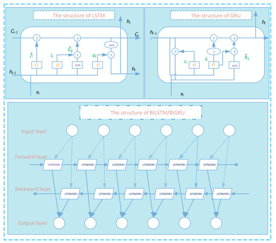
Figure 1.
Structure of BILSTM and BIGRU.
3. Overview of the Proposed Hybrid Method
3.1. Weighted Optimization System
In order to improve the prediction performance, BILSTM and BIGRU are introduced to predict at the same time. However, the mutual complementarity between these models must be optimized to take full advantage. Therefore, weighted optimization based on cuckoo search is carried out.
Cuckoo search is an optimization algorithm that can help improve prediction performance [41]. It resembles the cuckoo’s parasitic breeding conduct according to three main principals:
- (1)
- One cuckoo produces one egg and puts it into a random nest. This means that when the cuckoo search starts, it will first produce a random solution according to the objective function.
- (2)
- The best nest will be preserved for next sifting process. In the algorithm, new solutions are produced based on Lévy flight. Among all produced solutions, the best one will be preserved and the rest will be abandoned.
- (3)
- The number of the nest is regular, and the host can discriminate the egg at a probability of Ps ∈ [0, 1]. The algorithm will repeat the process until it meets the maximal generation, and give the best solution.
In the cuckoo search algorithm, the “eggs” are the possible solutions of the whole search, which means that each single solution is represented by the position of one egg in a host nest. Therefore, “nests” means a couple of solutions, and global search is equivalent to finding a nest and replacing the eggs in it, while local search means finding a new nest when the host bird detects the egg and abandons that nest. In fact, the cuckoo search combines local and global search. The quality of the egg, or the solution, is relevant to evaluating the indicator values of the objective function. The goal of the cuckoo search is to replace the existing solution with a better one, which is based on Lévy flight.
The movement of Lévy flight is a random walk under Lévy distribution. The mathematical expressions are as follows:
where represents the step size value; represents the ith location of the tth generation; means the ith location at the next generation; is the gamma function; and s and are the parameter values that determine the distribution of Lévy flight. The mathematical expression of the cuckoo search is as follows:
where H is the Heaviside function, is the step size value, ω is a random number drawn from a uniform distribution, P is the probability value to transmit among the local and global random walk, means the dot of each single element, and and are solutions picked randomly.
The algorithm principal of the weighted cuckoo search optimization, Algorithm 1, can be explained in brief. and represent the predicting result from BILSTM and BIGRU, is the value of final predicting result which is based on weighted optimization through cuckoo search. is the real value of stock index. In this paper, the parameters of the cuckoo search are given as follows: probability of finding eggs is 0.25; population is 25; maximum iteration is 100, step size is 0.1; Lévy exponent is 1.5.
| Algorithm 1 Principal of weighted cuckoo search optimization. | |
| Input: (prediction results of BILSTM), (prediction results of BIGRU), and (real points of stock index); number of iterations m, probability of finding eggs, number of population, value of step size, value of Lévy exponent Initialize: Randomly pick the set of a starting nest with (, ) Iteration I = 0 For i = 0, 1, …, m: 1. Generate w1 (weight of BILSTM prediction result) and w2 (weight of BIGRU prediction result), calculate (combined prediction result) and ei (performance criterion) 2. Compare ei with ei-1, replace the best nest with smaller error, update the combined prediction result 3. Replace the weights with the best nest, update the weights of BILSTM and BIGRU prediction results 4: Repeat steps 1 to 3 until iteration meets m, set the best nest with smallest prediction error Output: w1 and w2 | |
3.2. Structure of the Proposed Model
In pursuit of improved stock index prediction performance, a novel combined model is proposed in this paper. Figure 2 shows the framework of the proposed model. The design and the main steps of this model can be summarized in three stages:
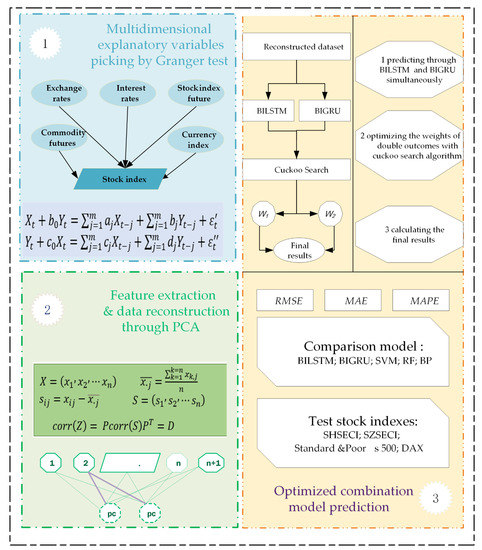
Figure 2.
Framework of proposed model.
- Feature extraction and data reconstruction. While multidimensional explanatory variables perform well with more data information, using them can cause setbacks in calculation because of data redundancy. In pursuit of easier calculation, transforming the original dataset is required. Hence, PCA is introduced next to extract features and transform the data, which will reduce data redundancy and improve the structure of the original multidimensional dataset.
- Prediction and optimization. For the predicting part, BILSTM and BIGRU are used separately to make predictions about the target stock index, the outcome of which lays a good foundation for the final shot. Then, the two outcomes from the models are optimized by cuckoo search, which can take advantage of both as well as provide mutual complementarity regarding precision and robustness. The final prediction outcome of the novel model is thus produced.
3.3. Evaluation Criteria
The evaluation criteria for prediction performance in this paper include RMSE, MAE, and MAPE, whose calculation formulas are given in Table 1. is the real value, while is the value of the prediction result.

Table 1.
Evaluation criteria.
4. Experiment
This section presents details on the data resources and the calculations for data transformation, the experimental criteria, and predictions.
4.1. Data Resource Descriptions
In this paper, four globally influential stock indices are chosen as targets for verification of model prediction effect and stability: SHSECI on the mainland, SZSECI on the mainland, Standard & Poor’s 500 in the USA, and DAX in Germany. The financial time series was from 15 August 2011 to 9 December 2020, among which 2392 trading numbers were proved effective after deleting invalid and unavailable numbers, such as asynchronous weekends, holidays, and trading days around the world. All data resources were downloaded from the website of East Money in China. The whole experiment is composed of three datasets: the training set accounts for 60%, the validation set 20%, and the testing set 20%. The data resources can be seen in Figure 3.
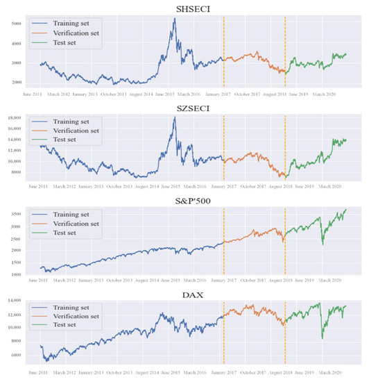
Figure 3.
Data resources.
4.2. Multidimensional Explanatory Variables
To make full use of external influences on stock index prediction, this paper introduces the Granger causality test to select potential relative variables from other markets. According to the results of past research and the Granger causality test, five main types of variables have an influence on stock index movement: exchange rates, stock index futures, interest rates, commodity futures, and currency index, as shown in Figure 4.
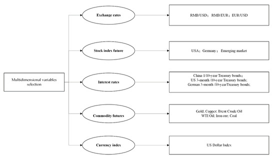
Figure 4.
Multidimensional variables.
4.3. Feature Extraction
In the process of data collection, data redundancy and insignificant information will reduce their effectiveness. Hence, it is necessary to find a way to extract features and reconstruct data so as to improve the data quality itself. This paper introduces principal component analysis to complete that task. The accumulated explained variance ratio is set above 99%. With the help of PCA, the data structure is transformed from high to low dimension without significant information loss, which undoubtedly greatly improves the data quality, improving the prediction performance. The outcomes of PCA are presented in Figure 5. Explained variance ratios are given in Table 2.
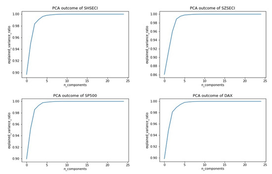
Figure 5.
Outcomes of PCA.
Table 2.
Explained variance ratio of four stock indices.
4.4. Empirical Results
This section presents the prediction performance of the proposed model and benchmark models.
Prediction and Comparisons
The prediction process of the hybrid model contains two steps. In step one, BILSTM and BIGRU make predictions individually at the same time, which provides two series as the prediction result for each one. In step two, the two prediction results are optimized by cuckoo search.
Apart from BILSTM and BIGRU, this paper also introduces support vector machine (SVM), random forest (RF), back propagation (BP), and a pure combination without Granger causality test and PCA (COMBINED) for comparison experiments to test the efficiency of the proposed model. In addition, we also designed different lag spans, serving as supplementary comparisons, to check the stability of model efficiency. There are six groups: 1, 3, 5, 7, 10, and 15 days. As a result, the whole experiment is composed of seven models plus six lag spans on four stock indices.
All experiments were tested on the platform of Jupyter Notebook with Python language. Table 3 shows all experiment errors. Apart from this, the group of 7-day lag experiments was chosen to give more information. Figure 6 shows a graph of the prediction performance. Figure 7 shows the prediction results. Table 4 shows comparisons of running times, Table 5 shows the weights of BILSTM and BIGRU, and Table 6 shows the outcomes of z-tests between proposed and benchmark models.
Table 3.
Prediction errors of four stock indices.
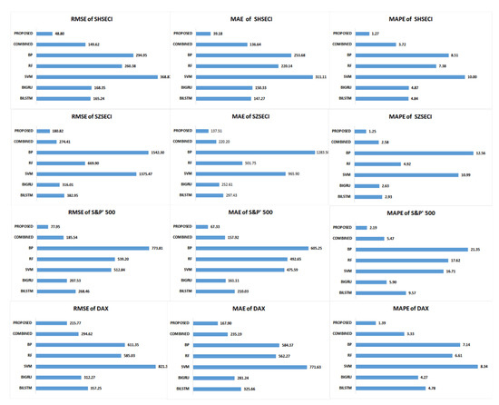
Figure 6.
Prediction performance of 7-day lag experiments.
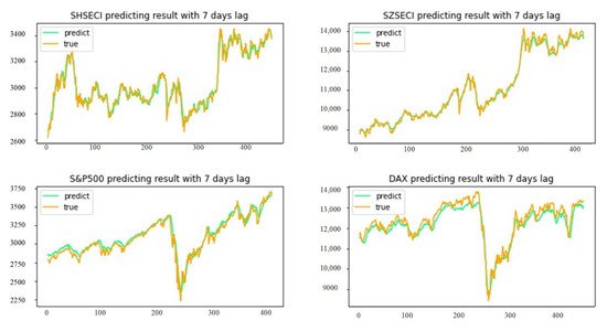
Figure 7.
Prediction results of four stock indices with 7-day lag.
Table 4.
Comparison of running time of 7-day lag experiments.
Table 5.
Weights of BILSTM and BIGRU (time lag = 7 days).
Table 6.
Outcomes of z-tests between proposed and benchmark models in 7-day lag experiments.
5. Results and Discussion
5.1. Results
With regard to the experimental results, it can be easily seen that the proposed model improves the prediction performance based on optimization, Granger causality test, and PCA. When it comes to prediction errors, the smaller the outcome, the better the prediction. It can be easily seen that the proposed model has better prediction performance.
5.2. Discussion
In the design, there are two dimensions for comparison in the experiment, one for verification of efficiency, and one for verification of stability. The prediction errors of the proposed model with different time lags in four stock markets are smaller than those of the benchmark models. When it comes to the test for efficiency, the prediction results of the proposed model on SHSECI, SZSECI, S&P 500, and DAX exceed those of benchmark models BILSTM, BIGRU, SVM, RF, BP, and COMBINED, which supports this point. When it comes to the test for stability, prediction results of different time lags provide proof.
The evaluation criteria in this paper are root mean square error, mean absolute error, and mean absolute percentage error, which are the widespread statistical criteria that can be seen in many papers. The prediction results are displayed in Table 3. With regard to the evaluation criteria, the proposed model has better prediction performance, which benefits from Granger causality test, PCA, and cuckoo search optimization. These comparison outcomes fully prove the effectiveness of the proposed model, and show its robustness for prediction of different stock markets in different situations. In this respect, the proposed model can be expected to be used for the prediction of other stock indices with better performance than benchmark models.
In order to give more comparison information, this paper chooses the 7-day lag to show the running times, weights, prediction situations, and z-test outcomes. The average running time is longer for the proposed model than other models. However, given the improved performance, the proposed model is worth using. In fact, different times series have different complexities, which makes it difficult for one single model to cover all prediction performance. The reason why the proposed model shows better performance than the other models is the use of the Granger causality test, PCA, and optimized weights. In other words, the Granger causality test and PCA can help to improve data quality, and cuckoo search takes advantage of both BILSTM and BIGRU, which can improve prediction performance.
From the comparisons above, the features of the proposed model are obvious. First, it is a good model that can be applied to different stock indices to make predictions. The comparison between four stock indices on seven benchmark models proves that. Second, the proposed model can be used to make predictions under different time lags. In other words, the model is robust to time lags, which helps to broaden its application.
To sum up, the proposed model is a good model for stock index prediction, which can improve prediction performance.
6. Conclusions
In order to improve the prediction of stock indices, a hybrid model based on optimization between BILSTM and BIGRU is proposed in this paper. This hybrid model first uses the Granger causality test to filter out the explanatory variables as much as possible. Then, it uses PCA to extract features of the multidimensional dataset to avoid data redundancy, which makes the prediction calculation easy and appropriate for common computers.
In the prediction process, two steps are designed. In step one, BILSTM and BIGRU make predictions individually at the same time. In step two, the outcomes of BILSTM and BIGRU are optimized through cuckoo search. The optimized prediction outcome represents the final prediction result of the proposed model in this paper. RMSE, MAE, and MAPE are introduced as evaluation criteria. With regard to these statistical errors, the proposed model successfully shows improved performance. In addition to the effectiveness test, the robustness result is also excellent. In short, from the point of view of comparison, the proposed model outperforms not only on different stock indices, but also on different time lags, which may bring opportunities for widespread application in stock index prediction.
All of the empirical evidence proves the excellence of the proposed model. However, the biggest contribution of this paper is regarding the exploration of combinations of different prediction models. Though the proposed model is a good start, there is still a long way to go in the pursuit of a better prediction model. For example, the best individual prediction model, combinations of three or more prediction models, and optimization algorithms have yet to be explored. Through consistent exploration, more and better prediction models will be developed, which will undoubtedly contribute a great deal to the whole prediction field.
Author Contributions
J.W., Y.L., Z.Z. and D.G.: conceived of the presented idea, developed the theory and performed the computations, discussed the results, wrote the paper, and approved the final manuscript. All authors have read and agreed to the published version of the manuscript.
Funding
This research was supported by the National Natural Science Foundation of China (Grant No. 71971122 and 71501101).
Institutional Review Board Statement
Not applicable.
Informed Consent Statement
Not applicable.
Data Availability Statement
Data used for this article is publicly available and collected from https://www.eastmoney.com (accessed on 1 September 2021).
Conflicts of Interest
The authors declare no conflict of interest.
Abbreviations
| PCA | Principal component analysis |
| SHSECI | Shanghai Stock Exchange Composite Index |
| SZSECI | Shenzhen Stock Exchange Components Index |
| ANN | Artificial neural network |
| ARMA | Autoregressive moving average |
| BILSTM | Bi-directional long short-term memory |
| BIGRU | Bi-directional gated recurrent unit |
| S&P 500 | Standard & Poor’s 500 |
| GARCH | Generalized autoregressive conditional heteroskedasticity |
| CEEMD | Complete ensemble empirical mode decomposition |
References
- Yamamoto, R. Predictor Choice, Investor Types, and the Price Impact of Trades on the Tokyo Stock Exchange. Comput. Econ. 2021. [Google Scholar] [CrossRef]
- Wang, Y.; Guo, Y.K. Forecasting Method of Stock Market Volatility in Time Series Data Based on Mixed Model of ARIMA and XGBoost. China Commun. 2020, 17, 205–221. [Google Scholar] [CrossRef]
- Rounaghi, M.M.; Zadeh, F.N. Investigation of market efficiency and Financial Stability between S&P 500 and London Stock Exchange: Monthly and yearly Forecasting of Time Series Stock Returns using ARMA model. Physical A 2016, 456, 10–21. [Google Scholar]
- Abounoori, E.; Elmi, Z.; Nademi, Y. Forecasting Tehran stock exchange volatility; Markov switching GARCH approach. Physical A 2016, 445, 264–282. [Google Scholar] [CrossRef]
- Barak, S.; Arjmand, A.; Ortobelli, S. Fusion of multiple diverse predictors in stock market. Inf. Fusion 2017, 36, 90–102. [Google Scholar] [CrossRef]
- Wang, Y.; Pan, Z.; Wu, C.; Wu, W. Industry equi-correlation: A powerful predictor of stock returns. J. Empir. Financ. 2020, 59, 1–24. [Google Scholar] [CrossRef]
- Qi, L. Technical analysis and stock return predictability: An aligned approach. J. Financ. Mark. 2018, 38, 103–123. [Google Scholar]
- Atsalakis, G.S.; Valavanis, P.K. Surveying stock market forecasting techniques—Part II: Soft computing methods. Expert Syst. Appl. 2008, 36, 5932–5941. [Google Scholar] [CrossRef]
- Wu, B.H.; Duan, T.T. A Performance Comparison of Neural Networks in Forecasting Stock Price Trend. Int. J. Comput. Intell. Syst. 2017, 10, 336–346. [Google Scholar] [CrossRef]
- Qiu, M.Y.; Song, Y.; Akagi, F. Application of artificial neural network for the prediction of stock market returns: The case of the Japanese stock market. Appl. Sci. Eng. 2016, 85, 1–7. [Google Scholar] [CrossRef]
- Liu, C.; Hou, W.Y.; Liu, D.Y. Foreign Exchange Rates Forecasting with Convolutional Neural Network. Neural Process. Lett. 2017, 46, 1095–1119. [Google Scholar] [CrossRef]
- Dutta, A.; Kumar, S.; Basu, M. A Gated Recurrent Unit Approach to Bitcoin Price Prediction. J. Risk Financ. Manag. 2020, 13, 23. [Google Scholar] [CrossRef]
- Kristjanpoller, W.; Minutolo, M.C. Gold price volatility: A forecasting approach using the Artificial Neural Network-GARCH model. Expert Syst. Appl. 2015, 40, 7245–7251. [Google Scholar] [CrossRef]
- Baffour, A.A.; Feng, J.C.; Taylor, E.K. A hybrid artificial neural network-GJR modeling approach to forecasting currency exchange rate volatility. Neurocomputing 2019, 365, 285–301. [Google Scholar] [CrossRef]
- Baek, Y.; Kim, H.Y. ModAugNet: A new forecasting framework for stock market index value with an overfitting prevention LSTM module and a prediction LSTM module. Expert Syst. Appl. 2018, 113, 457–480. [Google Scholar] [CrossRef]
- Alonso-Monsalve, S.; Suárez-Cetrulo, A.L.; Cervantes, A.; Quintana, D. Convolution on neural networks for high-frequency trend prediction of cryptocurrency exchange rates using technical indicators. Expert Syst. Appl. 2020, 149, 113250. [Google Scholar] [CrossRef]
- Kim, H.Y.; Won, C.H. Forecasting the volatility of stock price index: A hybrid model integrating LSTM with multiple GARCH-type models. Expert Syst. Appl. 2018, 103, 25–37. [Google Scholar] [CrossRef]
- Patil, S.; Mudaliar, V.M.; Kamat, P. LSTM based Ensemble Network to enhance the learning of long-term dependencies in chatbot. Int. J. Simul. Multidiscip. Des. Optim. 2020, 11, 25. [Google Scholar] [CrossRef]
- Lu, W.; Li, J.Z.; Wang, J.Y.; Qin, L.L. A CNN-BiLSTM-AM method for stock price prediction. Neural Comput. Appl. 2020, 33, 4741–4753. [Google Scholar] [CrossRef]
- Zhu, Q.; Zhang, F.; Liu, S. A hybrid VMD-BiGRU model for rubber futures time series forecasting. Appl. Soft Comput. 2019, 84, 105739. [Google Scholar] [CrossRef]
- Aslan, M.F.; Unlersen, M.F.; Sabanci, K.; Durdu, A. CNN-based transfer learning-BiLSTM network: A novel approach for COVID-19 infection detection. Appl. Soft Comput. J. 2021, 98, 106912. [Google Scholar] [CrossRef] [PubMed]
- Cao, J.; Li, Z.; Li, J. Financial time series forecasting model based on CEEMDAN and LSTM. Physical A 2019, 519, 127–139. [Google Scholar] [CrossRef]
- Yang, H.L.; Lin, H.C. Applying the Hybrid Model of EMD, PSR, and ELM to Exchange Rates Forecasting. Comput. Econ. 2017, 49, 99–116. [Google Scholar] [CrossRef]
- Yilanci, V.; Ozgur, O.; Gorus, M.S. Stock prices and economic activity nexus in OECD countries: New evidence from an asymmetric panel Granger causality test in the frequency domain. Financ. Innov. 2021, 7, 1–22. [Google Scholar] [CrossRef]
- Peng, T.F.; Chen, D.W.; Wei, P.B.; Yu, G.Y. Spillover effect and Granger causality investigation between China’s stock market and international oil market: A dynamic multiscale approach. J. Comput. Appl. Math. 2020, 367, 112460. [Google Scholar] [CrossRef]
- Chen, T.L.; Cheng, C.H.; Liu, J.W. A Causal Time-Series Model Based on Multilayer Perceptron Regression for Forecasting Taiwan Stock Index. Int. J. Inf. Technol. Decis. Mak. 2019, 18, 1967–1987. [Google Scholar] [CrossRef]
- Wang, L.; Ma, F.; Niu, T.J.; He, C.T. Crude oil and BRICS stock markets under extreme shocks: New evidence. Econ. Model. 2020, 86, 54–68. [Google Scholar] [CrossRef]
- Anowar, F.; Sadaoui, S.; Selim, B. Conceptual and empirical comparison of dimensionality reduction algorithms (PCA, KPCA, LDA, MDS, SVD, LLE, ISOMAP, LE, ICA, t-SNE). Comput. Sci. Rev. 2021, 40, 100378. [Google Scholar] [CrossRef]
- Chen, Y.J.; Hao, Y.J. Integrating principle component analysis and weighted support vector machine for stock trading signals prediction. Neurocomputing 2018, 321, 381–402. [Google Scholar] [CrossRef]
- Adnan, T.M.T.; Tanjim, M.M.; Adnan, M.A. Fast, scalable and geo-distributed PCA for big data analytics. Inf. Syst. 2021, 98, 101710. [Google Scholar] [CrossRef]
- Imanian, G.; Pourmina, M.A.; Salahi, A. Information-Based Node Selection for Joint PCA and Compressive Sensing-Based Data Aggregation. Wirel. Pers. Commun. 2021, 118, 1635–1654. [Google Scholar] [CrossRef]
- Li, Y. Multifractal view on China’s stock market crashes. Physical A 2019, 536, 122591. [Google Scholar] [CrossRef]
- Wang, Y.L. Stock market forecasting with financial micro-blog based on sentiment and time series analysis. J. Shanghai Jiaotong Univ. 2017, 22, 173–179. [Google Scholar] [CrossRef]
- Cheng, W.Y.; Wang, J. Nonlinear Fluctuation Behavior of Financial Time Series Model by Statistical Physics System. Abstr. Appl. Anal. 2014, 2014, 806271. [Google Scholar] [CrossRef]
- Tang, L.; Pan, H.; Yao, Y. EPAK: A Computational Intelligence Model for 2-level Prediction of Stock Indices. Int. J. Comput. Commun. Control 2018, 13, 268–279. [Google Scholar] [CrossRef][Green Version]
- Jia, Z.L.; Cui, M.L.; Li, H.D. Research on the relationship between the multifractality and long memory of realized volatility in the SSECI. Physical A 2012, 391, 740–749. [Google Scholar] [CrossRef]
- Rashid, A. Stock prices and trading volume: An assessment for linear and nonlinear Granger causality. J. Asian Econ. 2007, 18, 595–612. [Google Scholar] [CrossRef]
- Alzahrani, M.; Masih, M.; Omar, A.T. Linear and non-linear Granger causality between oil spot and futures prices: A wavelet-based test. J. Int. Money Financ. 2014, 48, 175–201. [Google Scholar] [CrossRef]
- Brūmelis, G.; Lapina, L.; Nikodemus, O.; Tabors, G. Use of an artificial model of monitoring data to aid interpretation of principal component analysis. Environ. Model. Softw. 2000, 15, 755–763. [Google Scholar] [CrossRef]
- Yan, B.H.; Han, G.D. LA-GRU: Building Combined Intrusion Detection Model Based on Imbalanced Learning and Gated Recurrent Unit Neural Network. Secur. Commun. Netw. 2018, 2018, 1–13. [Google Scholar] [CrossRef]
- Salgotra, R.; Singh, U.; Saha, S.; Gandomi, A.H. Self adaptive cuckoo search: Analysis and experimentation. Swarm Evol. Comput. 2021, 60, 100751. [Google Scholar] [CrossRef]


Publisher’s Note: MDPI stays neutral with regard to jurisdictional claims in published maps and institutional affiliations. |
© 2021 by the authors. Licensee MDPI, Basel, Switzerland. This article is an open access article distributed under the terms and conditions of the Creative Commons Attribution (CC BY) license (https://creativecommons.org/licenses/by/4.0/).