On PSO-Based Simulations of Fuzzy Dynamical Systems Induced by One-Dimensional Ones

Abstract

Zadeh’s extension principle is one of the elementary tools in fuzzy set theory, and among other things, it provides a natural extension of a real-valued continuous self-map to a self-map having fuzzy sets as its arguments. The purpose of this paper is to introduce a new algorithm that can be used for simulations of fuzzy dynamical systems induced by interval maps. The core of the proposed algorithm is based on calculations including piecewise linear maps, and consequently, an implementation of an optimization algorithm (in our case, particle swarm optimization) was prepared to obtain necessary piecewise linear approximations. For all parts of this algorithm, we provide detailed testing and numerous examples.

1. Introduction

Zadeh’s extension principle (known as Zadeh’s extension or an extension principle) is one of the most elementary tools in fuzzy theory. Roughly speaking, this principle says that a map $f:X\to Y$ induces another map $z_f:\mathbb{F}\left(X\right)\to \mathbb{F}\left(Y\right)$, where $\mathbb{F}\left(X\right)$ (resp. $\mathbb{F}\left(Y\right)$) is the family of fuzzy sets defined on X (resp. Y). This principle is naturally used in many areas of fuzzy mathematics such as fuzzy arithmetics, approximation reasoning, simulations, and even recently with the notion of interactivity incorporated [1,2]. To point out one particular application, we need to introduce the so-called discrete dynamical system. It is defined as a pair $(X,f)$, where X is a (usually topological) space and $f:X\to X$ is a continuous self-map. Then, Zadeh’s extension considered over a given discrete dynamical system $(X,f)$ induces a fuzzy (discrete) dynamical system (for details, we refer to the definitions in Section 1.3), which naturally incorporates and deals with the uncertainty of input states of x. There are theoretical results (e.g., [3] or recently [4] and the references therein) studying the mutual properties of the discrete dynamical system given by Zadeh’s extension principle.

1.1. Motivation of This Study

However, in practice and in full generality, the computation and approximation of Zadeh’s extension principle leads to a rather difficult task. The main reason is the difficult computation of the inverse of the map f under consideration. Only in a few specific cases (we refer to the text below), one can find an easier solution. Our approach provides a solution that is more general in several aspects.

1.2. State-of-the-Art

The problem of the approximation of Zadeh’s extension $z_f$ of $f:X\to X$ is well known, and many other authors have contributed to this issue, mostly under very specific assumptions and with no relation to dynamical system simulations. For example, several methods were elaborated for one-dimensional (interval) maps and fuzzy numbers only—e.g., in [5,6], a new method approximating $z_f\left(A\right)$, $A\in \mathbb{F}\left(X\right)$, based on the decomposition and multilinearization of a function f, was introduced. However, for one-dimensional systems and the extension to higher dimensions, this is computationally demanding [7]. Further, in [8], the authors proposed another method using an optimization over the $\alpha$-cuts of the fuzzy set, which should also ensure the convexity of the solution. Again, the computation was restricted to fuzzy numbers only. Moreover, in the latter papers, the trajectories of fuzzy dynamical systems were not considered and the approximation properties were not studied. Further, the usage of the parametric (LU-)representation of particular fuzzy numbers was proposed in [9] and even before in [10]. The LU-fuzzy representation is based on monotonic splines, which have flexible shapes, and it was claimed by the authors that it allows an easy and fast simulation of fuzzy dynamical systems, however, again, for fuzzy numbers only.

In [7], the authors proposed the so-called fuzzy calculator, which can approximate the membership output function (approximating Zadeh’s extension) of a continuous function, for which noninteractive input variables described by fuzzy intervals were considered, Therefore, the problem was transformed into several optimization problems (including particle swarm optimization) based on the $\alpha$-cut approach. These optimization algorithms were used to calculate the points of approximated $\alpha$-cuts, and then, under some assumptions, they could receive the first iteration of a fuzzy dynamical system. This is, to our best knowledge, the only approach that can be used so far for discrete dynamical systems of higher dimensions. However, the trajectory of a fuzzy dynamical system was not calculated here, and the optimization algorithms were used differently than in our approach. Moreover, this approach is different from the one presented in this manuscript: in our case, we do not use finite $\alpha$-cut representations, and therefore, we are able to distinguish nonconvex fuzzy sets in higher dimensions.

Thus, the practical approaches (mentioned above) are restricted to fuzzy numbers mostly and to the first application of Zadeh’s extension to the one-dimensional (interval) map in consideration. There is only one paper [9] in which several iterations of a given one-dimensional discrete dynamical system were experimentally computed, and this was performed for fuzzy numbers only. Our motivation was to prepare an algorithm avoiding these restrictions, i.e., to prepare a universal algorithm that will be flexible enough to simulate fuzzy dynamical system in which the input values will be represented not only by fuzzy numbers, which allows long-term simulations and, eventually, considering discrete dynamical systems in spaces of dimension greater than one.

There are also a few more theoretical works contributing to this topic. For instance, in [11], not only an interpolation technique (e.g., with the help of the F-transform) was published, but also the choice of the metric on the space of fuzzy sets and its effect on the expectation on the approximation were studied. For example, it has been shown that there are more suitable metrics than the standard, levelwise one. However, there has been no implementation of that proposal. Another paper [3] contributed to the theoretical background of the model of fuzzy dynamical systems induced by Zadeh’s extension principle, e.g., some topological properties of spaces of fuzzy sets or some continuity and convergence properties of generalized fuzzifications were surveyed and studied; additionally, the properties preserved by (semi-)conjugacies were specified. In another paper [12], the author elaborated on a very specific implementation of fuzzy arithmetics based on $\alpha$-cuts, which could prevent the possible widening of outcomes, but it cannot be implemented on any general map.

There are many related papers that should be mentioned, but we cannot comment on them properly due to the length of this manuscript. To provide a brief overview, one can find many papers on the approximations of fuzzy numbers [6,12,13], on practical implementations of the extension principle in real-world problems [14,15,16] (among others), or on the theoretical properties of fuzzy dynamical systems induced by the extension principle [17,18,19] (among others).

1.3. Novelties of This Study

The approach proposed in this manuscript is, in fact, a natural continuation and extension of two recent papers by the same authors. Recently, in [20], we introduced a preliminary version of the presented algorithm, dealing only with piecewise linear functions. Then, in [21], the next natural step, a generalization of the algorithm from [20] to an arbitrary continuous function, was briefly introduced with preliminary testing. We would like to emphasize that this manuscript fully extends and provides the readers with a fully extended testing.

In contrast to previous approaches (our approach can deal with more general classes of fuzzy sets (i.e., fuzzy sets, which are not fuzzy numbers)), we do not require any special fuzzy set representation, e.g., fuzzy sets to be necessarily fuzzy convex. It should be noted here that the convexity need not be preserved in higher dimensions. If needed, we are able to deal with the discontinuities of fuzzy sets, which naturally appear in trajectories of initial fuzzy states. Additionally, we also provide an implementation providing iterations of initial fuzzy states.

1.4. Additional Remarks

We would like to mention once more our previous algorithm [20] prepared for a distinct class of piecewise linear fuzzy sets, for which assuming the continuity is not necessary. This is an interesting feature because discontinuities naturally appear in simulations of fuzzy dynamical systems. The algorithm from [20] was able to deal with a much larger (i.e., topologically dense) class of interval maps. The approach presented in this manuscript significantly extends the computations to a whole class of all continuous one-dimensional (interval) maps (i.e., to the system of all continuous fuzzy sets). Another difference from previous approaches is that we already performed a preliminary testing of the quality approximation of some trajectories. We plan to develop this direction further, but before doing that, we need to test our algorithm on simpler cases, which is performed in this paper. Because of the famous butterfly effect, there will be a natural need to continuously adapt an approximation given by an evolutionary algorithm (that is why we used the PSO algorithm within this paper) and to allow further corrections of the studied trajectories.

The structure of this manuscript is the following. In the first section, basic terms from the fuzzy set theory related to metric spaces, dynamical systems, and fuzzy dynamical systems are introduced. In Section 2, the implementation of the particle swarm algorithm that is used for the linearization of interval (one-dimensional) functions is shown. The following section, i.e., Section 3, provides a discussion on the parameter selection of PSO-based linearizations. Finally, in Section 4, approximations of fuzzy dynamical systems are followed with a brief discussion on the precision and efficiency of the proposed algorithm (Section 5). Concluding remarks are given in Section 6.

1.5. Preliminaries

In this subsection, we introduce some basic notions used in our paper. For more information, we refer, for example, to [3,11].

Let $(X,d_X)$ be a nonempty metric space (sometimes called a universe). A fuzzy set A on a given metric space $(X,d_X)$ is a map $A:X\to [0,1]$, and for any point $x\in X$, the number $A\left(x\right)$ represents a membership degree of the point x in the fuzzy set A. A system of upper semicontinuous fuzzy sets in the universe X is denoted by $\mathbb{F}\left(X\right)$. The upper semicontinuity of fuzzy sets under consideration is not crucial for approximations, but it is formally required in the theoretical model of a discrete fuzzy dynamical system. Further, for $\alpha \in (0,1]$, the set ${\left[A\right]}_{\alpha }=\{x\in X\mid A\left(x\right)\ge \alpha \}$ is an α-cut of A. Note that a fuzzy set A is upper semicontinuous if and only if every $\alpha$-cut is a closed subset of X. A fuzzy set A is normal if $A\left(x\right)=1$ for some $x\in X$. Throughout this paper, we can expect that $X=[0,1]$, because the problem considered on many one-dimensional spaces can be easily reduced to this situation.

1.6. Metrics

Before we start with the definition of a discrete fuzzy dynamical system, we should define the notion of a metric on the space of fuzzy sets $\mathbb{F}\left(X\right)$. Such metrics are often computed with the help of a Hausdorff metric. Note that in the following text, $\epsilon$ is a real number, as usual. The Hausdorff metric $D_X$ between $A,B\in \mathbb{K}\left(X\right)$, where $\mathbb{K}\left(X\right)$ is a space of nonempty closed subsets of X, is defined by:

$$D_X(A,B)=inf\{\epsilon >0\mid A\subseteq U_{\epsilon }\left(B\right)\mathrm{and}B\subseteq U_{\epsilon }\left(A\right)\},$$

where:

$$U_{\epsilon }\left(A\right)=\{x\in X|D(x,A)<\epsilon \}.$$

Among the most often used metrics is the supremum metric $d_{\infty }$, defined as:

$$d_{\infty }(A,B)=\underset{\alpha \in (0,1]}{sup}{D}_X({\left[A\right]}_{\alpha },{\left[B\right]}_{\alpha }),$$

for $A,B\in \mathbb{F}\left(X\right).$ Other metrics, for example an endograph metric or sendograph metric, can be found in the literature [3]. These metrics are usually considered in connection with the topological structure on $\mathbb{F}\left(X\right)$.

However, in our algorithm introduced in Section 2, we need additional distance notions because we calculate the distance between an initial function and its piecewise linear approximation, and the metrics mentioned above are not suitable for this.

The distance between two finite vectors $\mathbf{x},\mathbf{y}$, which gives the sum of the lengths of the projections of the line segment between the points in coordinate axes, is a function $d_1:{\mathbb{R}}^q\times {\mathbb{R}}^q\to \mathbb{R}$ in q-dimensional space called $Manhattanmetric$. More precisely,

$$d_1(\mathbf{x},\mathbf{y})=\sum _{\mathbf{i}=\mathbf{1}}^{\mathbf{q}}|{\mathbf{x}}_{\mathbf{i}}-{\mathbf{y}}_{\mathbf{i}}|,$$

where $(\mathbf{x},\mathbf{y})$ are vectors $\mathbf{x}=(x_1,x_2,\cdots ,x_q)$, $\mathbf{y}=(y_1,y_2,\cdots ,y_q)$.

The distance between two vectors $\mathbf{x},\mathbf{y}$, that is assigned to arbitrary two vectors in q-dimensional space, is a function $d_2:{\mathbb{R}}^q\times {\mathbb{R}}^q\to \mathbb{R}$ called Euclidean metric. More precisely,

$$d_2(\mathbf{x},\mathbf{y})=\sqrt{{({\mathbf{x}}_{\mathbf{1}}-{\mathbf{y}}_{\mathbf{1}})}^{\mathbf{2}}+\cdots +{({\mathbf{x}}_{\mathbf{q}}-{\mathbf{y}}_{\mathbf{q}})}^{\mathbf{2}}},$$

where $(\mathbf{x},\mathbf{y})$ are vectors $\mathbf{x}=(x_1,x_2,\cdots ,x_q)$, $\mathbf{y}=(y_1,y_2,\cdots ,y_q)$.

A maximum metric (or Chebyshev distance) is a metric, often induced either by the supremum norm or uniform norm, defined in the following way:

$$d_3(\mathbf{x},\mathbf{y})=\underset{\mathbf{i}=\mathbf{1},\mathbf{2},\dots ,\mathbf{q}}{max}|{\mathbf{x}}_{\mathbf{i}}-{\mathbf{y}}_{\mathbf{i}}|,$$

where $(\mathbf{x},\mathbf{y})$ are vectors $\mathbf{x}=(x_1,x_2,\cdots ,x_q)$, $\mathbf{y}=(y_1,y_2,\cdots ,y_q)$.

1.7. Dynamical Systems

Let us briefly recall some elementary notions from topological dynamics (for details, we refer, e.g., to [22] and the references therein).

Assume now that X is a compact metric space and $f:X\to X$ is continuous. Then, a pair $(X,f)$ defines a (discrete) dynamical system. For any given initial state $x\in X$, we can consider a (forward) trajectory of x under the map f as an inductively defined sequence ${\left\{f^n\left(x\right)\right\}}_{n\in \mathbb{N}}$: $f^0\left(x\right)=x,f^1\left(x\right)=f\left(x\right)$ and $f^{n+1}\left(x\right)=f\left(f^n\left(x\right)\right)$ for every $n\in \mathbb{N}$. The initial state x we call a fixed point of the function f if $f\left(x\right)=x$. Similarly, the point $x\in X$ is called periodic if there exists $n\in \mathbb{N}$ such that $f^n\left(x\right)=x$. These notions are briefly demonstrated in the following example.

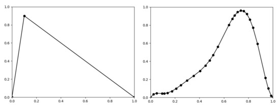
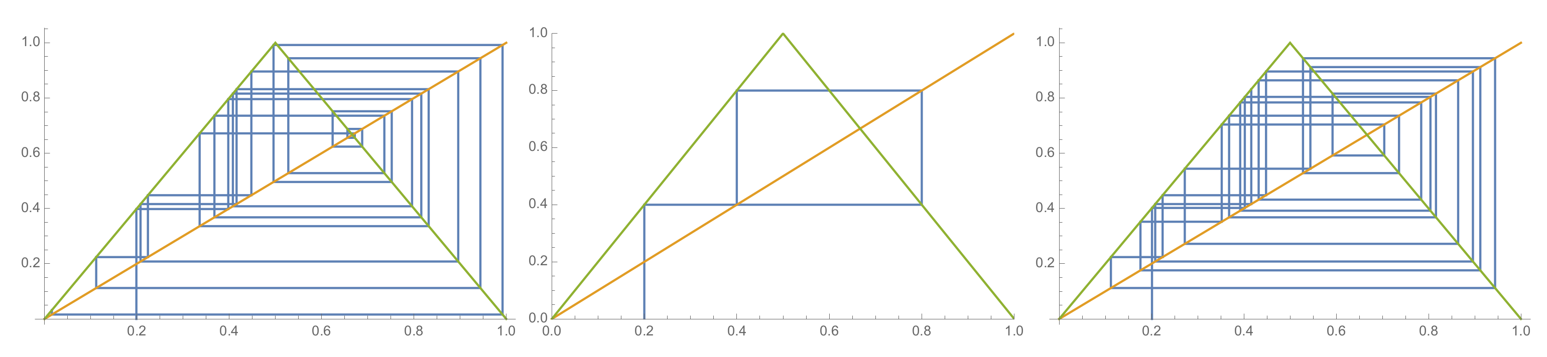
Example 1.

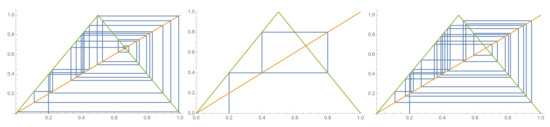
Let us consider a tent map T, where $T:[0,1]\to [0,1]$ is defined by

$T\left(x\right)=\left\{\begin{array}{cc}2x,\hfill & 0\le x<1/2,\hfill \\ 2(1-x),\hfill & 1/2\le x\le 1.\hfill \end{array}\right.$

In Figure 1, one can easily see that $T\left(0\right)=0$ (i.e., 0 is a fixed point), $0.2$ is eventually periodic (the middle picture below), which means that the trajectory of $0.2$ becomes periodic in a finitely many iterations. Finally, $0.4$ (and hence, $0.8$) is a periodic point with period 2.

Figure 1. Trajectories of three initial states around the value $0.2$ of the dynamical system given by the tent map.

1.8. Fuzzy Dynamical Systems

We are ready to define a fuzzy dynamical system given by Zadeh’s extension principle, first defined by Zadeh in 1975 [23].

Consider now a discrete dynamical system $(X,f)$. The map $f:X\to X$ defines another map $z_f:\mathbb{F}\left(X\right)\to \mathbb{F}\left(X\right)$ defined on the space of fuzzy sets $\mathbb{F}\left(X\right)$ by the following formula:

$$\left(z_f\left(A\right)\right)\left(x\right)=\underset{y\in f^{-1}\left(x\right)}{sup}\left\{A\left(y\right)\right\}.$$

Naturally, $\left(z_f\left(A\right)\right)\left(x\right)=0$ whenever $f^{-1}=\varnothing$. Then, the map $z_f$ is a fuzzification (or Zadeh’s extension) of the map $f:X\to X$. There are many facts known for $z_f$; see, e.g., [3,24] and the references therein. For instance, an intuition of how $z_f$ works can be provided by: ${\left[z_f\left(A\right)\right]}_{\alpha }=f\left({\left[A\right]}_{\alpha }\right)$ for any $A\in \mathbb{F}\left(X\right)$ and $\alpha \in (0,1]$.

It is also known that the continuity of $f:X\to X$ implies the continuity of the fuzzification $z_f:\mathbb{F}\left(X\right)\to \mathbb{F}\left(X\right)$ with respect to the metric topology given by the levelwise metric $d_{\infty }$ (and also other metrics). Consequently, $(\mathbb{F}\left(X\right),z_f)$ is correctly defined as a discrete fuzzy dynamical system. For more information, we refer to [3].

Example 2.

To present some dynamical systems, we refer to some examples below. Namely, a few first iterations of Zadeh’s extensions of functions ($g_1$, $g_2$ and $g_3$) (Section 4.2) are depicted in Figures 6–11.

2. Particle Swarm Optimization

In this subsection, we recall Particle Swarm Optimization (PSO), which is one of the evolutionary algorithms based on repetitive stochastic input adaptation, which is inspired by the social behavior of the species (R. Eberhart and J. Kennedy in 1995 [25,26]).

Let us briefly demonstrate the use of the PSO algorithm for searching a global optimum of an interval map $f:[0,1]\to [0,1]$. At the very beginning, we establish a population of a finite set, say of $n\in \mathbb{N}$ points $x\in [0,1]$ called particles. In the subsequent steps, the population is firstly evaluated, and then, each particle moves in the domain, where movements are influenced by its historical behavior and, very often, also by neighboring particles. The process is combined together with the help of the choice of stochastic parameters (acceleration coefficients, constriction factor), adapted towards the required solution.

Our implementation of the PSO algorithm above is the following: we search for a linearization $l_f$ (see the definition of a piecewise linear function below) of a fixed interval map $f:[0,1]\to [0,1]$. To find a suitable solution, a function to be minimized is a distance function between f and its possible linearization $l_f$. Therefore, because every possible linearization can be represented by a finite number, say $\ell \in \mathbb{N}$, of points, every population consists of n particles represented by ℓ-dimensional vectors, and all, stochastic, parameters are adapted accordingly. The details of this construction are mentioned in the following pseudocode (Section 2.1).

Throughout this paper, we work with piecewise linear functions; thus, the definition of a piecewise linear function should be mentioned. A continuous interval map $f:[0,1]\to [0,1]$ is called piecewise linear provided there are finitely many points ${\left\{c_i\right\}}_{i=1}^{\ell }\subseteq [0,1]$, $0=c_1<c_2<\dots <c_{\ell }=1$, such that ${f|}_{[c_i,c_{i+1}]}$ is linear for every $i=1,2,\dots ,\ell -1$. Obviously, a piecewise linear function f can be uniquely defined by finitely many pairs $(c_i,s_i)\in [0,1]\times [0,1]$, for $i=1,\cdots ,\ell$, if the turning points $c_i$ preserve the ordering above.

2.1. Pseudocode of PSO-Based Linearization

A pseudocode of the proposed algorithm consists of seven steps:

• Initialization:
  • A continuous function $f:[0,1]\to [0,1]$;
  • $\ell \in \mathbb{N}$ indicates a dimension of the problem and a number $\ell -1$ of linear segments of the approximating function;
  • A particle is a vector $\mathbf{x}\in {[0,1]}^{\ell }$, where $\mathbf{x}=(x_1,x_2,\cdots ,x_{\ell })$ and all $x_i$s are pairwise different;
  • $n\in \mathbb{N}$ denotes a number of particles;
  • Thus, $Part={\left\{{\mathbf{x}}^i\right\}}_{i=1}^n,P={\left\{{\mathbf{p}}^i\right\}}_{i=1}^n$ are finite sets of vectors ${\mathbf{x}}^i,{\mathbf{p}}^i\in {[0,1]}^{\ell }$. At the beginning, $Part,P$ are randomly chosen particles;
  • For every particle $\mathbf{x}=(x_1,x_2,\cdots ,x_{\ell })$, a general formula for (piecewise linear) function ${Pl}_{\mathbf{x}}:[0,1]\to [0,1]$ given by ℓ pairs $(x_i,f\left(x_i\right))$ is the following:
    ${Pl}_x\left(x\right)=\left\{\begin{array}{cc}f\left(x_1\right)+(f\left(x_2\right)-f\left(x_1\right))\frac{(x-x_1)}{(x_2-x_1)},\hfill & x_1\le x\le x_2,\hfill \\ f\left(x_2\right)+(f\left(x_3\right)-f\left(x_2\right))\frac{(x-x_2)}{(x_3-x_2)},\hfill & x_2\le x\le x_3,\hfill \\ ⋮\hfill \\ f\left(x_{\ell -1}\right)+(f\left(x_{\ell }\right)-f\left(x_{\ell -1}\right))\frac{(x-x_{\ell -1})}{(x_l-x_{\ell -1})},\hfill & x_{\ell -1}\le x\le x_{\ell };\hfill \end{array}\right.$
  • $D={\left\{d_m\right\}}_{m=1}^q\subseteq [0,1]$, such that $0=d_1<d_2<\cdots <d_q=1$, is a set of equidistant points on the interval $[0,1]$;
  • A chosen metric is denoted by M;
  • $V={\left\{{\mathbf{v}}^i\right\}}_{i=1}^n$ is a set of vectors ${\mathbf{v}}^i\in {[0,1]}^{\ell }$, where $\mathbf{v}$ is the velocity of each particle. Let the initial velocities ${\mathbf{v}}_i$ be zero vectors, i.e., ${\mathbf{v}}_i$$=(0,0,\cdots ,0)$ for every i;
  • ${\mathit{U}}_{{\mathsf{\Phi }}_1}={\left\{{\mathbf{U}}_{{\mathsf{\Phi }}_1}^i\right\}}_{i=1}^n\subseteq {[0,{\mathsf{\Phi }}_1]}^{\ell }$, ${\mathit{U}}_{{\mathsf{\Phi }}_2}={\left\{{\mathbf{U}}_{{\mathsf{\Phi }}_2}^i\right\}}_{i=1}^n\subseteq {[0,{\mathsf{\Phi }}_2]}^{\ell }$ are sets of vectors with uniform distributions from intervals $(0,{\mathsf{\Phi }}_1)$, $(0,{\mathsf{\Phi }}_2)$, where ${\mathsf{\Phi }}_1$, ${\mathsf{\Phi }}_2$ are called acceleration coefficients;
  • $\chi \in \mathbb{R}$ is called a constriction factor;
  • A number of iterations $I\in \mathbb{N}$;
• Distances:
  • For all ${\mathbf{x}}^I\in Part$, where $I=1,\cdots ,n$, calculate $DIst\left({\mathbf{x}}^I\right)=M(f,{Pl}_{{\mathrm{x}}^I},D)$ (i.e., we calculate a distance M between two functions f and $P{l}_{{\mathbf{x}}^I}$ at finitely many points D for every particle ${\mathbf{x}}^I$), and denoted ${\mathbf{P}}_{\mathbf{best}}=\{{\mathbf{P}}_{{\mathbf{best}}_2},{\mathbf{P}}_{{\mathbf{best}}_2},\cdots ,{\mathbf{P}}_{{\mathbf{best}}_n}\}$;
  • For all ${\mathbf{p}}^I\in P$, where $I=1,\cdots ,n$, calculate ${\mathbf{P}}_{\mathbf{best}I}=M(f,{Pl}_{{\mathbf{p}}^I},D)$, where M is a given metric, and from that, ${\mathbf{P}}_{\mathbf{best}}=\{{\mathbf{P}}_{{\mathbf{best}}_1},{\mathbf{P}}_{{\mathbf{best}}_2},\cdots ,{\mathbf{P}}_{{\mathbf{best}}_n}\}$;
• Comparison:
  • Compare elements from Dist and P_best such that for all $I=1,\cdots ,n$, if ${DIst}_I\le {\mathbf{P}}_{\mathbf{best}I}$, then ${\mathbf{P}}_{\mathbf{best}I}:={DIst}_I$, otherwise ${\mathbf{P}}_{\mathbf{best}I}:={\mathbf{P}}_{\mathbf{best}I}$;
• Best neighbors:
  • There exists $k_1$ such that ${DIst}_{k_1}\le {DIst}_j$, where $j=\{1,2,\cdots ,n\}\setminus \left\{k_1\right\}$, and $k_2$ such that ${DIst}_{k_2}\le {DIst}_j$, where $j=\{1,2,\cdots ,n\}\setminus \{k_1,k_2\}$, and assign them vectors ${\mathbf{x}}^{k_1}$, ${\mathbf{x}}^{k_2}$ from Part;
  • Create a set ${\mathbf{P}}^{\mathrm{g}}={\left\{{\mathbf{p}}_g^I\right\}}_{I=1}^n$, ${\mathbf{p}}_g^I\in {[0,1]}^{\ell }$ (called the set of best neighbors), where at the position $k_2$ is a vector ${\mathbf{x}}^{k_2}\in Part$ and everywhere else is vector ${\mathbf{x}}^{k_1}\in Part$;
• Calculation:
  • For all $I=1,\cdots ,n$, calculate the velocity ${\mathbf{v}}^I$ and update the set Part of particles ${\mathbf{x}}^I$:

    –

    ${\mathbf{v}}^I:=\chi ({\mathbf{v}}^I+{\mathbf{U}}_{{\mathsf{\Phi }}_1}({\mathbf{p}}^I-{\mathbf{x}}^I)+{\mathbf{U}}_{{\mathsf{\Phi }}_2}({\mathbf{p}}_g^I-{\mathbf{x}}^I))$, where ${\mathbf{U}}_{{\mathsf{\Phi }}_1}$ and ${\mathbf{U}}_{{\mathsf{\Phi }}_2}$ are random vectors (defined above) embedding a piece of randomness in every step of the algorithm (There is no relationship between ${\mathbf{U}}_{{\mathsf{\Phi }}_1}$ and ${\mathbf{U}}_{{\mathsf{\Phi }}_2}$ at the very beginning. However, mutual choices of ${\mathsf{\Phi }}_1$ and ${\mathsf{\Phi }}_2$ can influence the quality of the output, and this feature is studied later in this manuscript.);

    –

    ${\mathbf{x}}^I:={\mathbf{x}}^I+{\mathbf{v}}^I$;

  • If the number I is not achieved, then continue with Step 2, otherwise go to Step 6.
• The best particle:
  • For the finite set $Part={\left\{{\mathbf{x}}^I\right\}}_{I=1}^n$, calculate $DIst\left({\mathbf{x}}^I\right)=M(f,{Pl}_{{\mathrm{x}}^I},D)$. Thus, $\mathbf{Dist}=\{{DIst}_1,{DIst}_2,\cdots ,{DIst}_n\}$;
  • There exists an element $k_1$ such that ${DIst}_{k1}\le {DIst}_j$, where $j=\{1,2,\cdots ,n\}\setminus \left\{k_1\right\}$, and assign it a vector ${\mathbf{x}}^{k_1}$ from Part to obtain the best distribution of points for a given function;
  • Calculate $f\left({\mathbf{x}}^{k_1}\right)$;
• Output:
  • Set of pairs $({\mathbf{x}}^{k_1},f\left({\mathbf{x}}^{k_1}\right))$ giving the best possible linearization $l_f$ of a function f.

3. Testing of the Linearization Procedure

In this section, we discuss some of the parameters which can affect the linearization procedure. After that, we introduce functions used for testing, and at the end of this section, we provide a summary of the results of the algorithm accuracy given by means and standard deviations.

3.1. Parameter Selection

Naturally, the PSO parameters choice can have a significant impact on optimization performance. In our optimization algorithm, we search for an appropriate setting of the constriction factor $\chi$ and the acceleration coefficients ${\mathsf{\Phi }}_1,{\mathsf{\Phi }}_2$. The parameter ${\mathsf{\Phi }}_1$ is the personal best value and, ${\mathsf{\Phi }}_2$ is the best neighbors value. In the case that values of both parameters are high, the velocity can grow up faster, and, consequently, the algorithm can be unstable, but there is a need to get to know the behavior of the proposed parameter in particular tasks. It is known that the equation $\mathsf{\Phi }={\mathsf{\Phi }}_1+{\mathsf{\Phi }}_2$, where $\mathsf{\Phi }>4$, should be satisfied and the authors recommended ${\mathsf{\Phi }}_1,{\mathsf{\Phi }}_2$ set to 2.05. Parameter $\chi$ is not changed during the algorithm run, it has a restrictive effect on the result. In the original version [26], PSO works with $\chi =2/\left(\mathsf{\Phi }-2+\sqrt{{\mathsf{\Phi }}^2-4\mathsf{\Phi }}\right)$.

For our purpose, we were testing which combination of parameters can be the most appropriate, so we chose $\chi =\{0.57,0.61,0.65,0.69,0.73\}$ and ${\mathsf{\Phi }}_1,{\mathsf{\Phi }}_2=\{1.65,1.85,2.05,2.25,2.45\}$. For each of five testing function (see (1)–(5) below) and parameter selection, the result was calculated 50 times. Additionally, we set $\ell =12$, $D=80$, $n=25$ and $I=100$. These parameters are chosen only for our testing purposes, thus before using the proposed algorithm one should always consider, which parameters to choose according to functions and spaces in consideration. For example in the case of interval maps, the number of linear parts should be bigger than the number of monotone parts of the function. The distances between the initial (linearized) function and the approximating (linearizing) piecewise linear function are given with the help of metrics introduced in Section 1.6.

3.2. Functions Used for Testing

To be able to test this algorithm, we chose the following functions (see Figure 2), trying to consider them from simpler ones to a very complex one:

$$f_1\left(x\right)=4x(1-x)$$

(1)

$$f_2\left(x\right)=\frac{1}{2}\left(\frac{sin(\left(\frac{3}{2}\right)}{x+\frac{1}{10})}+1\right)$$

(2)

$$f_3\left(x\right)=\frac{1}{25}\left(sin20x+20x·sin20x·cos20x\right)+\frac{1}{2}$$

(3)

$$\begin{array}{c}\hfill f_4\left(x\right)=0.9+(-1+x)(0.9+(-0.16+(5.4+(-27+(36+(510+\\ \hfill (-120-2560(-0.9+x\left)\right)(-0.1+x)\left)\right(-0.6+x\left)\right)\\ \hfill (-0.2+x)\left)\right(-0.8+x\left)\right)(-0.4+x)\left)x\right)\end{array}$$

(4)

$$f_5\left(x\right)=\left(x-\frac{1}{2}\right)\left(sin\frac{1}{x-\frac{1}{2}}\right)+\frac{1}{2}$$

(5)

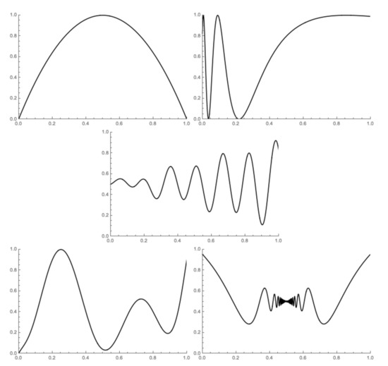
Figure 2. The graphs of the functions $f_{\left(1\right)}$, $f_{\left(2\right)}$, $f_{\left(3\right)}$, $f_{\left(4\right)}$, and $f_{\left(5\right)}$.

It follows from Section 3.1 that for each of these functions, we considered 125 combinations of parameters $\chi$, ${\mathsf{\Phi }}_1$, ${\mathsf{\Phi }}_2$; for each of these combinations, we repeated 25 runs, and the outcomes were evaluated with the help of three metrics. The conclusion of our statistical testing is provided in the next subsection.

3.3. The Choice of Parameters: Our Conclusion

In this subsection, we do not show all the obtained results due to the fact that this manuscript would be too long. However, we would like to present our general observations obtained for interval maps.

For demonstration purposes, we show the results of the mean and standard deviation for functions $f_1$ (see Table 1, Table 2 and Table 3) and $f_4$ (see Table 4, Table 5 and Table 6), which are the most suitable functions to use for our chosen parameter setting. In these tables, three types of metrics, twenty-five combinations of ${\mathsf{\Phi }}_1,{\mathsf{\Phi }}_2$, and five different values of $\chi$ are used. Naturally, the choice of parameter $\chi$ can affect the final result. In general, we recommend using values $\chi \in [0.57,0.69]$. It turned out from our testing that if $\chi$ was smaller than $0.57$, the results were not convincing, and on the other hand, the same happened if $\chi$ was bigger than 0.69. We can find more effective combinations of ${\mathsf{\Phi }}_1,{\mathsf{\Phi }}_2$, but the best combinations were mostly given when ${\mathsf{\Phi }}_1$ was greater than ${\mathsf{\Phi }}_2$.

Table 1. The values of the arithmetic mean and standard deviation of $f_1$ obtained using PSO with $I=100,D=80,$$\ell =12$, $n=25$ for 50 calculations with the metric $d_1$.

$\mathit{\chi }$	${\mathsf{\Phi }}_1=1.65,{\mathsf{\Phi }}_2=1.65$	${\mathsf{\Phi }}_1=1.65,{\mathsf{\Phi }}_2=2.05$	${\mathsf{\Phi }}_1=1.65,{\mathsf{\Phi }}_2=2.45$	${\mathsf{\Phi }}_1=2.05,{\mathsf{\Phi }}_2=2.05$	${\mathsf{\Phi }}_1=2.05,{\mathsf{\Phi }}_2=2.45$
0.57	0.44673 ± 0.00954	0.44384 ± 0.00711	0.44651 ± 0.01313	0.44135 ± 0.00568	0.44421 ± 0.00696
0.61	0.44713 ± 0.01215	0.44373 ± 0.00739	0.44093 ± 0.00422	0.44489 ± 0.00951	0.44153 ± 0.00582
0.65	0.44306 ± 0.00762	0.44317 ± 0.01346	0.43962 ± 0.00271	0.44082 ± 0.00664	0.44156 ± 0.00449
0.69	0.44195 ± 0.00687	0.44086 ± 0.00518	0.46219 ± 0.03799	0.43999 ± 0.00298	0.47689 ± 0.05146
0.73	0.44079 ± 0.00615	0.45020 ± 0.01613	0.57076 ± 0.09284	0.46718 ± 0.03999	0.64096 ± 0.12199
0.57	0.44355 ± 0.00961	0.44265 ± 0.00589	0.44357 ± 0.0072	0.44675 ± 0.01298	0.44597 ± 0.01079
0.61	0.44329 ± 0.01365	0.44249 ± 0.00833	0.44606 ± 0.0126	0.44398 ± 0.00775	0.44399 ± 0.00721
0.65	0.44589 ± 0.01372	0.44101 ± 0.00461	0.44171 ± 0.0053	0.44338 ± 0.00705	0.44310 ± 0.00761
0.69	0.53436 ± 0.09852	0.44438 ± 0.01404	0.44102 ± 0.0042	0.44065 ± 0.00464	0.44319 ± 0.01528
0.73	0.69188 ± 0.12316	0.51971 ± 0.07506	0.44457 ± 0.0123	0.44112 ± 0.00611	0.44109 ± 0.00463
$\chi$	${\mathsf{\Phi }}_1=1.65,{\mathsf{\Phi }}_2=2.25$	${\mathsf{\Phi }}_1=1.85,{\mathsf{\Phi }}_2=1.85$	${\mathsf{\Phi }}_1=1.85,{\mathsf{\Phi }}_2=2.05$	${\mathsf{\Phi }}_1=1.85,{\mathsf{\Phi }}_2=2.25$	${\mathsf{\Phi }}_1=1.85,{\mathsf{\Phi }}_2=2.45$
0.57	0.44299 ± 0.00882	0.44486 ± 0.00942	0.44398 ± 0.00721	0.44505 ± 0.01220	0.44572 ± 0.00972
0.61	0.44239 ± 0.00657	0.44524 ± 0.01199	0.44343 ± 0.00778	0.44311 ± 0.00764	0.44292 ± 0.00789
0.65	0.44116 ± 0.00677	0.44115 ± 0.00566	0.44281 ± 0.00832	0.44112 ± 0.00590	0.44088 ± 0.00432
0.69	0.44378 ± 0.01419	0.44162 ± 0.00589	0.44027 ± 0.00392	0.44333 ± 0.01879	0.46286 ± 0.03899
0.73	0.49788 ± 0.06003	0.44165 ± 0.00504	0.45538 ± 0.01999	0.49800 ± 0.05539	0.59158 ± 0.09469
$\chi$	${\mathsf{\Phi }}_1=2.05,{\mathsf{\Phi }}_2=2.25$	${\mathsf{\Phi }}_1=2.25,{\mathsf{\Phi }}_2=2.25$	${\mathsf{\Phi }}_1=2.25,{\mathsf{\Phi }}_2=2.45$	${\mathsf{\Phi }}_1=2.45,{\mathsf{\Phi }}_2=2.25$	${\mathsf{\Phi }}_1=2.45,{\mathsf{\Phi }}_2=1.85$
0.57	0.44485 ± 0.00773	0.44334 ± 0.00829	0.44387 ± 0.00856	0.44495 ± 0.01425	0.44402 ± 0.01057
0.61	0.44507 ± 0.01544	0.44187 ± 0.00656	0.44056 ± 0.00452	0.44194 ± 0.00601	0.44251 ± 0.00724
0.65	0.43928 ± 0.00283	0.44065 ± 0.00343	0.44204 ± 0.01235	0.44051 ± 0.00434	0.44099 ± 0.00562
0.69	0.44618 ± 0.01709	0.45029 ± 0.01819	0.48591 ± 0.06187	0.47058 ± 0.04682	0.44028 ± 0.00408
0.73	0.54212 ± 0.07472	0.57070 ± 0.09529	0.63198 ± 0.11265	0.60194 ± 0.08960	0.46416 ± 0.03948
$\chi$	${\mathsf{\Phi }}_1=2.25,{\mathsf{\Phi }}_2=2.05$	${\mathsf{\Phi }}_1=2.25,{\mathsf{\Phi }}_2=1.85$	${\mathsf{\Phi }}_1=2.25,{\mathsf{\Phi }}_2=1.65$	${\mathsf{\Phi }}_1=2.05,{\mathsf{\Phi }}_2=1.85$	${\mathsf{\Phi }}_1=1.85,{\mathsf{\Phi }}_2=1.65$
0.57	0.44339 ± 0.00751	0.44268 ± 0.0069	0.44485 ± 0.00868	0.44525 ± 0.00901	0.44481 ± 0.0069
0.61	0.44326 ± 0.00879	0.44267 ± 0.0069	0.44431 ± 0.00840	0.44217 ± 0.00600	0.44447 ± 0.0098
0.65	0.44159 ± 0.00586	0.44208 ± 0.0067	0.44129 ± 0.00605	0.44161 ± 0.00803	0.44404 ± 0.0079
0.69	0.44158 ± 0.00441	0.44146 ± 0.0059	0.44002 ± 0.00434	0.44189 ± 0.01391	0.44150 ± 0.0051
0.73	0.50101 ± 0.06959	0.44738 ± 0.01114	0.44264 ± 0.01486	0.44507 ± 0.01224	0.44012 ± 0.0039

Table 2. The values of mean and standard deviation of $f_1$ obtained using PSO with $I=100,D=80,\ell =12,n=25$ for 50 calculations with the metric $d_2$.

$\mathit{\chi }$	${\mathsf{\Phi }}_1=1.65,{\mathsf{\Phi }}_2=1.65$	${\mathsf{\Phi }}_1=1.65,{\mathsf{\Phi }}_2=2.05$	${\mathsf{\Phi }}_1=1.65,{\mathsf{\Phi }}_2=2.45$	${\mathsf{\Phi }}_1=2.05,{\mathsf{\Phi }}_2=2.05$	${\mathsf{\Phi }}_1=2.05,{\mathsf{\Phi }}_2=2.45$
0.57	0.05529 ± 0.00187	0.05586 ± 0.00264	0.05570 ± 0.00275	0.05515 ± 0.00168	0.05489 ± 0.00151
0.61	0.05513 ± 0.00141	0.05508 ± 0.00186	0.05422 ± 0.00043	0.05443 ± 0.00074	0.05409 ± 0.00015
0.65	0.05460 ± 0.00096	0.05437 ± 0.00162	0.05410 ± 0.00023	0.05436 ± 0.00161	0.05422 ± 0.00026
0.69	0.05418 ± 0.00043	0.05412 ± 0.00022	0.05824 ± 0.00727	0.05492 ± 0.00269	0.06171 ± 0.00799
0.73	0.05411 ± 0.00028	0.05554 ± 0.00318	0.07709 ± 0.01397	0.05954 ± 0.00644	0.08721 ± 0.01525
$\chi$	${\mathsf{\Phi }}_1=2.45,{\mathsf{\Phi }}_2=2.45$	${\mathsf{\Phi }}_1=2.45,{\mathsf{\Phi }}_2=2.05$	${\mathsf{\Phi }}_1=2.45,{\mathsf{\Phi }}_2=1.65$	${\mathsf{\Phi }}_1=2.05,{\mathsf{\Phi }}_2=1.65$	${\mathsf{\Phi }}_1=1.65,{\mathsf{\Phi }}_2=1.85$
0.57	0.05456 ± 0.00107	0.05507 ± 0.00195	0.05511 ± 0.00131	0.05555 ± 0.00225	0.05589 ± 0.00293
0.61	0.05432 ± 0.00161	0.05469 ± 0.00175	0.05475 ± 0.0011	0.05485 ± 0.00139	0.05495 ± 0.00131
0.65	0.05573 ± 0.00338	0.05418 ± 0.00036	0.05471 ± 0.0018	0.05462 ± 0.00123	0.05463 ± 0.00096
0.69	0.07252 ± 0.01461	0.05500 ± 0.00131	0.05415 ± 0.0003	0.05442 ± 0.00163	0.05437 ± 0.00161
0.73	0.09237 ± 0.02132	0.06873 ± 0.01340	0.05477 ± 0.0008	0.05421 ± 0.00038	0.05431 ± 0.00063
$\chi$	${\mathsf{\Phi }}_1=1.65,{\mathsf{\Phi }}_2=2.25$	${\mathsf{\Phi }}_1=1.85,{\mathsf{\Phi }}_2=1.85$	${\mathsf{\Phi }}_1=1.85,{\mathsf{\Phi }}_2=2.05$	${\mathsf{\Phi }}_1=1.85,{\mathsf{\Phi }}_2=2.25$	${\mathsf{\Phi }}_1=1.85,{\mathsf{\Phi }}_2=2.45$
0.57	0.05559 ± 0.00264	0.05511 ± 0.00114	0.05535 ± 0.00218	0.05521 ± 0.00160	0.05518 ± 0.00173
0.61	0.05496 ± 0.00187	0.05518 ± 0.00189	0.05499 ± 0.00196	0.05476 ± 0.00193	0.05428 ± 0.00061
0.65	0.05509 ± 0.00308	0.05444 ± 0.00178	0.05419 ± 0.00038	0.05497 ± 0.00309	0.05483 ± 0.00269
0.69	0.05447 ± 0.00074	0.05435 ± 0.00160	0.05462 ± 0.00224	0.05470 ± 0.00076	0.05876 ± 0.00712
0.73	0.06186 ± 0.00892	0.05471 ± 0.00149	0.05669 ± 0.00412	0.06832 ± 0.01121	0.08204 ± 0.01479
0.57	0.05493 ± 0.00133	0.05517 ± 0.00193	0.05460 ± 0.00099	0.05478 ± 0.00183	0.05487 ± 0.0011
0.61	0.05428 ± 0.00053	0.05419 ± 0.00034	0.05481 ± 0.00269	0.05445 ± 0.00107	0.05440 ± 0.0008
0.65	0.05435 ± 0.00158	0.05448 ± 0.00162	0.05468 ± 0.00163	0.05426 ± 0.00039	0.05429 ± 0.0006
0.69	0.05587 ± 0.00439	0.05646 ± 0.00377	0.06490 ± 0.00903	0.05964 ± 0.00694	0.05454 ± 0.0016
0.73	0.07375 ± 0.01268	0.07905 ± 0.01679	0.09397 ± 0.01939	0.08506 ± 0.01829	0.05756 ± 0.00459
$\chi$	${\mathsf{\Phi }}_1=2.25,{\mathsf{\Phi }}_2=2.05$	${\mathsf{\Phi }}_1=2.25,{\mathsf{\Phi }}_2=1.85$	${\mathsf{\Phi }}_1=2.25,{\mathsf{\Phi }}_2=1.65$	${\mathsf{\Phi }}_1=2.05,{\mathsf{\Phi }}_2=1.85$	${\mathsf{\Phi }}_1=1.85,{\mathsf{\Phi }}_2=1.65$
0.57	0.05521 ± 0.00193	0.05549 ± 0.00198	0.05533 ± 0.00242	0.05563 ± 0.00207	0.05609 ± 0.00289
0.61	0.05442 ± 0.00075	0.05446 ± 0.00066	0.05479 ± 0.0012	0.05501 ± 0.00192	0.05559 ± 0.00257
0.65	0.05409 ± 0.00018	0.05417 ± 0.00033	0.05439 ± 0.0007	0.05425 ± 0.00044	0.05445 ± 0.00090
0.69	0.05439 ± 0.00053	0.05419 ± 0.00032	0.05416 ± 0.0004	0.05459 ± 0.00222	0.05412 ± 0.00027
0.73	0.06403 ± 0.01104	0.05679 ± 0.00633	0.05431 ± 0.0005	0.05513 ± 0.00217	0.05439 ± 0.00160

Table 3. The values of mean and standard deviation of $f_1$ obtained using PSO with $I=100,D=80,\ell =12,n=25$ for 50 calculations with the metric $d_3$.

$\mathit{\chi }$	${\mathsf{\Phi }}_1=1.65,{\mathsf{\Phi }}_2=1.65$	${\mathsf{\Phi }}_1=1.65,{\mathsf{\Phi }}_2=2.05$	${\mathsf{\Phi }}_1=1.65,{\mathsf{\Phi }}_2=2.45$	${\mathsf{\Phi }}_1=2.05,{\mathsf{\Phi }}_2=2.05$	${\mathsf{\Phi }}_1=2.05,{\mathsf{\Phi }}_2=2.45$
0.57	0.01054 ± 0.00109	0.01014 ± 0.00096	0.01048 ± 0.00128	0.00999 ± 0.00101	0.01031 ± 0.00132
0.61	0.01046 ± 0.00139	0.00997 ± 0.00114	0.01002 ± 0.00118	0.00970 ± 0.00105	0.00977 ± 0.00115
0.65	0.01000 ± 0.00092	0.00983 ± 0.00109	0.01006 ± 0.00090	0.00978 ± 0.00107	0.01034 ± 0.00136
0.69	0.00978 ± 0.00109	0.00967 ± 0.00129	0.01367 ± 0.00287	0.01081 ± 0.00206	0.01677 ± 0.00382
0.73	0.00993 ± 0.00102	0.01417 ± 0.00373	0.02092 ± 0.00360	0.01694 ± 0.00395	0.02359 ± 0.00474
$\chi$	${\mathsf{\Phi }}_1=2.45,{\mathsf{\Phi }}_2=2.45$	${\mathsf{\Phi }}_1=2.45,{\mathsf{\Phi }}_2=2.05$	${\mathsf{\Phi }}_1=2.45,{\mathsf{\Phi }}_2=1.65$	${\mathsf{\Phi }}_1=2.05,{\mathsf{\Phi }}_2=1.65$	${\mathsf{\Phi }}_1=1.65,{\mathsf{\Phi }}_2=1.85$
0.57	0.00990 ± 0.00115	0.01012 ± 0.00149	0.01019 ± 0.00095	0.01034 ± 0.00099	0.01032 ± 0.00139
0.61	0.00960 ± 0.00082	0.00989 ± 0.00119	0.01013 ± 0.0012	0.01026 ± 0.00105	0.01009 ± 0.00139
0.65	0.01234 ± 0.00258	0.00983 ± 0.00092	0.00960 ± 0.0009	0.00985 ± 0.0011	0.00992 ± 0.00096
0.69	0.01908 ± 0.00399	0.01227 ± 0.00244	0.00954 ± 0.0008	0.00995 ± 0.0012	0.00956 ± 0.00104
0.73	0.02447 ± 0.00545	0.02009 ± 0.00495	0.01243 ± 0.00285	0.00986 ± 0.0008	0.01041 ± 0.00160
$\chi$	${\mathsf{\Phi }}_1=1.65,{\mathsf{\Phi }}_2=2.25$	${\mathsf{\Phi }}_1=1.85,{\mathsf{\Phi }}_2=1.85$	${\mathsf{\Phi }}_1=1.85,{\mathsf{\Phi }}_2=2.05$	${\mathsf{\Phi }}_1=1.85,{\mathsf{\Phi }}_2=2.25$	${\mathsf{\Phi }}_1=1.85,{\mathsf{\Phi }}_2=2.45$
0.57	0.01049 ± 0.00124	0.01048 ± 0.00150	0.01009 ± 0.00106	0.01025 ± 0.00138	0.01002 ± 0.00107
0.61	0.00993 ± 0.00104	0.01016 ± 0.00101	0.01007 ± 0.00101	0.00986 ± 0.00129	0.00986 ± 0.00129
0.65	0.00990 ± 0.00106	0.00965 ± 0.00083	0.00985 ± 0.00127	0.00978 ± 0.00122	0.01038 ± 0.00162
0.69	0.01073 ± 0.00159	0.00954 ± 0.00097	0.00975 ± 0.00092	0.01229 ± 0.00262	0.01514 ± 0.00371
0.73	0.01749 ± 0.00491	0.01114 ± 0.00218	0.01614 ± 0.00456	0.01933 ± 0.00450	0.02248 ± 0.00508
$\chi$	${\mathsf{\Phi }}_1=2.05,{\mathsf{\Phi }}_2=2.25$	${\mathsf{\Phi }}_1=2.25,{\mathsf{\Phi }}_2=2.25$	${\mathsf{\Phi }}_1=2.25,{\mathsf{\Phi }}_2=2.45$	${\mathsf{\Phi }}_1=2.45,{\mathsf{\Phi }}_2=2.25$	${\mathsf{\Phi }}_1=2.45,{\mathsf{\Phi }}_2=1.85$
0.57	0.01017 ± 0.00109	0.01016 ± 0.00111	0.01018 ± 0.00115	0.00988 ± 0.00112	0.01009 ± 0.0010
0.61	0.00976 ± 0.00102	0.00981 ± 0.00109	0.00959 ± 0.00092	0.00948 ± 0.00085	0.00978 ± 0.0011
0.65	0.00996 ± 0.00116	0.01002 ± 0.00095	0.01141 ± 0.00198	0.01079 ± 0.00181	0.00959 ± 0.0009
0.69	0.01255 ± 0.00250	0.01424 ± 0.00355	0.01795 ± 0.00421	0.01615 ± 0.00384	0.01027 ± 0.00119
0.73	0.02044 ± 0.00514	0.02101 ± 0.00434	0.02369 ± 0.00486	0.02190 ± 0.00482	0.01581 ± 0.00469
$\chi$	${\mathsf{\Phi }}_1=2.25,{\mathsf{\Phi }}_2=2.05$	${\mathsf{\Phi }}_1=2.25,{\mathsf{\Phi }}_2=1.85$	${\mathsf{\Phi }}_1=2.25,{\mathsf{\Phi }}_2=1.65$	${\mathsf{\Phi }}_1=2.05,{\mathsf{\Phi }}_2=1.85$	${\mathsf{\Phi }}_1=1.85,{\mathsf{\Phi }}_2=1.65$
0.57	0.01030 ± 0.00092	0.01015 ± 0.00136	0.01029 ± 0.00108	0.01029 ± 0.00118	0.01061 ± 0.00116
0.61	0.00991 ± 0.00085	0.00970 ± 0.00083	0.00983 ± 0.00117	0.01038 ± 0.00135	0.01001 ± 0.00091
0.65	0.00961 ± 0.00100	0.00961 ± 0.00091	0.00961 ± 0.00096	0.00979 ± 0.00108	0.00989 ± 0.00107
0.69	0.01127 ± 0.00209	0.00963 ± 0.00092	0.00973 ± 0.00092	0.00958 ± 0.00113	0.00950 ± 0.00101
0.73	0.01746 ± 0.00515	0.01386 ± 0.00279	0.01075 ± 0.00211	0.01209 ± 0.00271	0.01008 ± 0.00094

Table 4. The values of mean and standard deviation of $f_4$ obtained using PSO with $I=100,D=80,\ell =12,n=25$ for 50 calculations with the metric $d_1$.

$\mathit{\chi }$	${\mathsf{\Phi }}_1=1.65,{\mathsf{\Phi }}_2=1.65$	${\mathsf{\Phi }}_1=1.65,{\mathsf{\Phi }}_2=2.05$	${\mathsf{\Phi }}_1=1.65,{\mathsf{\Phi }}_2=2.45$	${\mathsf{\Phi }}_1=2.05,{\mathsf{\Phi }}_2=2.05$	${\mathsf{\Phi }}_1=2.05,{\mathsf{\Phi }}_2=2.45$
0.57	1.59037 ± 0.24984	1.62977 ± 0.23772	1.60976 ± 0.21587	1.57976 ± 0.22699	1.59274 ± 0.19044
0.61	1.57176 ± 0.25262	1.64725 ± 0.22590	1.58791 ± 0.24802	1.56674 ± 0.24249	1.55923 ± 0.18462
0.65	1.62446 ± 0.23553	1.58594 ± 0.24937	1.55904 ± 0.21288	1.56094 ± 0.22623	1.56596 ± 0.18687
0.69	1.59593 ± 0.28093	1.57662 ± 0.22099	1.62292 ± 0.23394	1.53793 ± 0.20723	1.82780 ± 0.48461
0.73	1.54296 ± 0.18417	1.62974 ± 0.40005	2.18634 ± 0.67657	1.86329 ± 0.53715	2.81114 ± 0.71643
$\chi$	${\mathsf{\Phi }}_1=2.45,{\mathsf{\Phi }}_2=2.45$	${\mathsf{\Phi }}_1=2.45,{\mathsf{\Phi }}_2=2.05$	${\mathsf{\Phi }}_1=2.45,{\mathsf{\Phi }}_2=1.65$	${\mathsf{\Phi }}_1=2.05,{\mathsf{\Phi }}_2=1.65$	${\mathsf{\Phi }}_1=1.65,{\mathsf{\Phi }}_2=1.85$
0.57	1.54953 ± 0.18691	1.56018 ± 0.23274	1.54420 ± 0.2148	1.59272 ± 0.22315	1.56309 ± 0.19567
0.61	1.60100 ± 0.24606	1.58447 ± 0.23445	1.52752 ± 0.1661	1.54771 ± 0.22381	1.64471 ± 0.23448
0.65	1.58873 ± 0.19722	1.56955 ± 0.19748	1.53435 ± 0.1962	1.55929 ± 0.20766	1.62295 ± 0.23805
0.69	2.11355 ± 0.62874	1.57120 ± 0.21650	1.58346 ± 0.2232	1.57702 ± 0.22283	1.54543 ± 0.21958
0.73	3.08575 ± 0.76636	2.12823 ± 0.63962	1.61309 ± 0.30878	1.55072 ± 0.19665	1.54910 ± 0.19549
$\chi$	${\mathsf{\Phi }}_1=1.65,{\mathsf{\Phi }}_2=2.25$	${\mathsf{\Phi }}_1=1.85,{\mathsf{\Phi }}_2=1.85$	${\mathsf{\Phi }}_1=1.85,{\mathsf{\Phi }}_2=2.05$	${\mathsf{\Phi }}_1=1.85,{\mathsf{\Phi }}_2=2.25$	${\mathsf{\Phi }}_1=1.85,{\mathsf{\Phi }}_2=2.45$
0.57	1.56249 ± 0.26237	1.58887 ± 0.19827	1.53361 ± 0.19833	1.63057 ± 0.23101	1.64117 ± 0.25050
0.61	1.64186 ± 0.25542	1.62414 ± 0.28323	1.60212 ± 0.20032	1.55226 ± 0.18392	1.62043 ± 0.20008
0.65	1.58061 ± 0.25445	1.56751 ± 0.20445	1.54011 ± 0.18398	1.52378 ± 0.19117	1.60934 ± 0.23505
0.69	1.64619 ± 0.24111	1.58701 ± 0.23610	1.55877 ± 0.20568	1.59617 ± 0.21269	1.77919 ± 0.50372
0.73	1.83898 ± 0.41817	1.57396 ± 0.22158	1.75303 ± 0.48211	1.98592 ± 0.62888	2.55976 ± 0.88166
$\chi$	${\mathsf{\Phi }}_1=2.05,{\mathsf{\Phi }}_2=2.25$	${\mathsf{\Phi }}_1=2.25,{\mathsf{\Phi }}_2=2.25$	${\mathsf{\Phi }}_1=2.25,{\mathsf{\Phi }}_2=2.45$	${\mathsf{\Phi }}_1=2.45,{\mathsf{\Phi }}_2=2.25$	${\mathsf{\Phi }}_1=2.45,{\mathsf{\Phi }}_2=1.85$
0.57	1.62477 ± 0.23632	1.59425 ± 0.23888	1.64423 ± 0.23898	1.59602 ± 0.19285	1.56970 ± 0.20420
0.61	1.62939 ± 0.22346	1.62814 ± 0.25448	1.59375 ± 0.22899	1.58834 ± 0.21454	1.53290 ± 0.19722
0.65	1.54596 ± 0.20629	1.52123 ± 0.20487	1.53762 ± 0.20138	1.54952 ± 0.22325	1.56256 ± 0.20221
0.69	1.58287 ± 0.25216	1.56052 ± 0.17442	2.02994 ± 0.68198	1.69919 ± 0.28745	1.49550 ± 0.16993
0.73	2.13561 ± 0.58176	2.44483 ± 0.84383	2.83623 ± 0.75432	2.79640 ± 0.76496	1.81328 ± 0.57589
$\chi$	${\mathsf{\Phi }}_1=2.25,{\mathsf{\Phi }}_2=2.05$	${\mathsf{\Phi }}_1=2.25,{\mathsf{\Phi }}_2=1.85$	${\mathsf{\Phi }}_1=2.25,{\mathsf{\Phi }}_2=1.65$	${\mathsf{\Phi }}_1=2.05,{\mathsf{\Phi }}_2=1.85$	${\mathsf{\Phi }}_1=1.85,{\mathsf{\Phi }}_2=1.65$
0.57	1.55519 ± 0.19483	1.54445 ± 0.1999	1.59542 ± 0.24518	1.61905 ± 0.24451	1.619185 ± 0.2652
0.61	1.57253 ± 0.24238	1.56136 ± 0.1877	1.55255 ± 0.21057	1.58888 ± 0.20543	1.56638 ± 0.1918
0.65	1.58877 ± 0.20531	1.52698 ± 0.1733	1.59913 ± 0.21885	1.58028 ± 0.23733	1.56697 ± 0.2314
0.69	1.57858 ± 0.23933	1.53281 ± 0.2015	1.49796 ± 0.19331	1.52631 ± 0.20260	1.56326 ± 0.2191
0.73	1.86237 ± 0.55692	1.61428 ± 0.22193	1.55055 ± 0.20346	1.53991 ± 0.20199	1.57203 ± 0.20965

Table 5. The values of mean and standard deviation of $f_4$ obtained using PSO with $I=100,D=80,\ell =12,n=25$ for 50 calculations with the metric $d_2$.

$\mathit{\chi }$	${\mathsf{\Phi }}_1=1.65,{\mathsf{\Phi }}_2=1.65$	${\mathsf{\Phi }}_1=1.65,{\mathsf{\Phi }}_2=2.05$	${\mathsf{\Phi }}_1=1.65,{\mathsf{\Phi }}_2=2.45$	${\mathsf{\Phi }}_1=2.05,{\mathsf{\Phi }}_2=2.05$	${\mathsf{\Phi }}_1=2.05,{\mathsf{\Phi }}_2=2.45$
0.57	0.22428 ± 0.04796	0.22339 ± 0.04519	0.23525 ± 0.05531	0.22591 ± 0.04513	0.22228 ± 0.04359
0.61	0.22588 ± 0.04931	0.22616 ± 0.04679	0.24263 ± 0.04674	0.21206 ± 0.03926	0.21532 ± 0.03998
0.65	0.21930 ± 0.04664	0.22361 ± 0.05068	0.23316 ± 0.04788	0.22258 ± 0.04518	0.22230 ± 0.04847
0.69	0.22161 ± 0.04589	0.22314 ± 0.04748	0.22553 ± 0.04635	0.23269 ± 0.04760	0.26191 ± 0.06652
0.73	0.22129 ± 0.04425	0.22577 ± 0.04872	0.35671 ± 0.11336	0.24843 ± 0.07165	0.40197 ± 0.10584
$\chi$	${\mathsf{\Phi }}_1=2.45,{\mathsf{\Phi }}_2=2.45$	${\mathsf{\Phi }}_1=2.45,{\mathsf{\Phi }}_2=2.05$	${\mathsf{\Phi }}_1=2.45,{\mathsf{\Phi }}_2=1.65$	${\mathsf{\Phi }}_1=2.05,{\mathsf{\Phi }}_2=1.65$	${\mathsf{\Phi }}_1=1.65,{\mathsf{\Phi }}_2=1.85$
0.57	0.21494 ± 0.04212	0.22804 ± 0.05293	0.21972 ± 0.0456	0.22398 ± 0.04644	0.22409 ± 0.04693
0.61	0.22228 ± 0.04269	0.22473 ± 0.05040	0.22697 ± 0.0477	0.22819 ± 0.04674	0.22183 ± 0.04719
0.65	0.21996 ± 0.04131	0.21865 ± 0.04135	0.21537 ± 0.0394	0.22257 ± 0.04993	0.22894 ± 0.04954
0.69	0.30814 ± 0.09305	0.22586 ± 0.04540	0.20867 ± 0.0379	0.21307 ± 0.03884	0.22351 ± 0.04718
0.73	0.47047 ± 0.08969	0.30696 ± 0.08766	0.22502 ± 0.05328	0.20869 ± 0.03358	0.22016 ± 0.04894
0.57	0.23748 ± 0.05018	0.22955 ± 0.04986	0.22928 ± 0.05013	0.24323 ± 0.04934	0.23398 ± 0.04834
0.61	0.23593 ± 0.05504	0.23270 ± 0.05155	0.22148 ± 0.04521	0.23444 ± 0.04959	0.24798 ± 0.05103
0.65	0.21569 ± 0.04623	0.23239 ± 0.04840	0.22238 ± 0.04693	0.22163 ± 0.04204	0.21798 ± 0.04421
0.69	0.23198 ± 0.04504	0.23036 ± 0.04744	0.23554 ± 0.04707	0.22059 ± 0.05076	0.25991 ± 0.07731
0.73	0.26495 ± 0.08492	0.23875 ± 0.05508	0.24165 ± 0.06436	0.30658 ± 0.10267	0.34796 ± 0.11848
$\chi$	${\mathsf{\Phi }}_1=2.05,{\mathsf{\Phi }}_2=2.25$	${\mathsf{\Phi }}_1=2.25,{\mathsf{\Phi }}_2=2.25$	${\mathsf{\Phi }}_1=2.25,{\mathsf{\Phi }}_2=2.45$	${\mathsf{\Phi }}_1=2.45,{\mathsf{\Phi }}_2=2.25$	${\mathsf{\Phi }}_1=2.45,{\mathsf{\Phi }}_2=1.85$
0.57	0.23759 ± 0.05529	0.22647 ± 0.04859	0.23110 ± 0.04822	0.21771 ± 0.03847	0.22337 ± 0.04781
0.61	0.23447 ± 0.05261	0.21992 ± 0.04422	0.21165 ± 0.04038	0.22259 ± 0.04845	0.21999 ± 0.0426
0.65	0.22119 ± 0.04488	0.21702 ± 0.04438	0.22111 ± 0.04777	0.21502 ± 0.04317	0.20878 ± 0.0381
0.69	0.22634 ± 0.04375	0.24130 ± 0.06648	0.29621 ± 0.09594	0.26973 ± 0.07975	0.22204 ± 0.0504
0.73	0.29735 ± 0.08863	0.37698 ± 0.11345	0.44674 ± 0.14117	0.42936 ± 0.14449	0.27860 ± 0.09009
$\chi$	${\mathsf{\Phi }}_1=2.25,{\mathsf{\Phi }}_2=2.05$	${\mathsf{\Phi }}_1=2.25,{\mathsf{\Phi }}_2=1.85$	${\mathsf{\Phi }}_1=2.25,{\mathsf{\Phi }}_2=1.65$	${\mathsf{\Phi }}_1=2.05,{\mathsf{\Phi }}_2=1.85$	${\mathsf{\Phi }}_1=1.85,{\mathsf{\Phi }}_2=1.65$
0.57	0.23532 ± 0.04658	0.23531 ± 0.04888	0.22888 ± 0.04673	0.22384 ± 0.04304	0.22043 ± 0.04402
0.61	0.22432 ± 0.04966	0.21942 ± 0.04624	0.21421 ± 0.0417	0.22569 ± 0.04689	0.22739 ± 0.04739
0.65	0.21499 ± 0.03993	0.21576 ± 0.04011	0.20710 ± 0.0357	0.21864 ± 0.04639	0.21948 ± 0.05028
0.69	0.22334 ± 0.04574	0.20707 ± 0.03682	0.21833 ± 0.0420	0.22015 ± 0.04512	0.21713 ± 0.04304
0.73	0.28392 ± 0.09143	0.23115 ± 0.06359	0.21731 ± 0.0458	0.22633 ± 0.05611	0.21560 ± 0.04133

Table 6. The values of mean and standard deviation of $f_4$ obtained using PSO with $I=100,D=80,\ell =12,n=25$ for 50 calculations with the metric $d_3$.

$\mathit{\chi }$	${\mathsf{\Phi }}_1=1.65,{\mathsf{\Phi }}_2=1.65$	${\mathsf{\Phi }}_1=1.65,{\mathsf{\Phi }}_2=2.05$	${\mathsf{\Phi }}_1=1.65,{\mathsf{\Phi }}_2=2.45$	${\mathsf{\Phi }}_1=2.05,{\mathsf{\Phi }}_2=2.05$	${\mathsf{\Phi }}_1=2.05,{\mathsf{\Phi }}_2=2.45$
0.57	0.05884 ± 0.01919	0.05521 ± 0.01975	0.06012 ± 0.02065	0.05911 ± 0.02112	0.05146 ± 0.01865
0.61	0.05671 ± 0.01967	0.05254 ± 0.01905	0.05957 ± 0.02184	0.05166 ± 0.01809	0.05355 ± 0.01981
0.65	0.05706 ± 0.02057	0.05382 ± 0.01959	0.05499 ± 0.02002	0.05379 ± 0.02009	0.05977 ± 0.01951
0.69	0.05141 ± 0.01956	0.05742 ± 0.02228	0.07635 ± 0.02211	0.05969 ± 0.02245	0.09168 ± 0.02804
0.73	0.05623 ± 0.02020	0.07677 ± 0.03276	0.10688 ± 0.02519	0.08755 ± 0.02855	0.11951 ± 0.02804
$\chi$	${\mathsf{\Phi }}_1=2.45,{\mathsf{\Phi }}_2=2.45$	${\mathsf{\Phi }}_1=2.45,{\mathsf{\Phi }}_2=2.05$	${\mathsf{\Phi }}_1=2.45,{\mathsf{\Phi }}_2=1.65$	${\mathsf{\Phi }}_1=2.05,{\mathsf{\Phi }}_2=1.65$	${\mathsf{\Phi }}_1=1.65,{\mathsf{\Phi }}_2=1.85$
0.57	0.05688 ± 0.02054	0.05567 ± 0.02012	0.05074 ± 0.0161	0.05686 ± 0.01921	0.05817 ± 0.01892
0.61	0.05426 ± 0.01928	0.05532 ± 0.02062	0.04914 ± 0.0162	0.05955 ± 0.02080	0.05128 ± 0.01757
0.65	0.06146 ± 0.01945	0.05346 ± 0.01897	0.05201 ± 0.0195	0.05321 ± 0.0195	0.05467 ± 0.01963
0.69	0.11293 ± 0.03684	0.06863 ± 0.02501	0.05464 ± 0.0207	0.04997 ± 0.0183	0.05359 ± 0.02032
0.73	0.13540 ± 0.03379	0.11486 ± 0.02767	0.06863 ± 0.02962	0.05769 ± 0.02018	0.05972 ± 0.02053
$\chi$	${\mathsf{\Phi }}_1=1.65,{\mathsf{\Phi }}_2=2.25$	${\mathsf{\Phi }}_1=1.85,{\mathsf{\Phi }}_2=1.85$	${\mathsf{\Phi }}_1=1.85,{\mathsf{\Phi }}_2=2.05$	${\mathsf{\Phi }}_1=1.85,{\mathsf{\Phi }}_2=2.25$	${\mathsf{\Phi }}_1=1.85,{\mathsf{\Phi }}_2=2.45$
0.57	0.05581 ± 0.01955	0.05344 ± 0.01804	0.05749 ± 0.02033	0.05290 ± 0.01914	0.06272 ± 0.02081
0.61	0.05822 ± 0.02049	0.05653 ± 0.01924	0.05368 ± 0.02003	0.05748 ± 0.02183	0.05149 ± 0.01913
0.65	0.05626 ± 0.02037	0.05522 ± 0.02034	0.06168 ± 0.02261	0.05604 ± 0.02044	0.05319 ± 0.01736
0.69	0.06797 ± 0.02293	0.05133 ± 0.01934	0.06178 ± 0.02204	0.06414 ± 0.01960	0.07969 ± 0.02570
0.73	0.10082 ± 0.02886	0.06129 ± 0.02273	0.08309 ± 0.02806	0.09859 ± 0.02905	0.11416 ± 0.02832
$\chi$	${\mathsf{\Phi }}_1=2.05,{\mathsf{\Phi }}_2=2.25$	${\mathsf{\Phi }}_1=2.25,{\mathsf{\Phi }}_2=2.25$	${\mathsf{\Phi }}_1=2.25,{\mathsf{\Phi }}_2=2.45$	${\mathsf{\Phi }}_1=2.45,{\mathsf{\Phi }}_2=2.25$	${\mathsf{\Phi }}_1=2.45,{\mathsf{\Phi }}_2=1.85$
0.57	0.05549 ± 0.02101	0.05338 ± 0.01915	0.05483 ± 0.01977	0.05722 ± 0.02035	0.04985 ± 0.0158
0.61	0.05290 ± 0.01891	0.05442 ± 0.01984	0.06215 ± 0.02202	0.04994 ± 0.01849	0.04707 ± 0.0154
0.65	0.05358 ± 0.02055	0.05709 ± 0.01980	0.06311 ± 0.02427	0.05655 ± 0.02084	0.05245 ± 0.0193
0.69	0.06777 ± 0.02369	0.07196 ± 0.02419	0.09635 ± 0.03088	0.09084 ± 0.03178	0.06001 ± 0.02202
0.73	0.10526 ± 0.02582	0.12179 ± 0.03535	0.13492 ± 0.03662	0.12453 ± 0.02500	0.08574 ± 0.03117
$\chi$	${\mathsf{\Phi }}_1=2.25,{\mathsf{\Phi }}_2=2.05$	${\mathsf{\Phi }}_1=2.25,{\mathsf{\Phi }}_2=1.85$	${\mathsf{\Phi }}_1=2.25,{\mathsf{\Phi }}_2=1.65$	${\mathsf{\Phi }}_1=2.05,{\mathsf{\Phi }}_2=1.85$	${\mathsf{\Phi }}_1=1.85,{\mathsf{\Phi }}_2=1.65$
0.57	0.05076 ± 0.01727	0.05409 ± 0.01944	0.05397 ± 0.01721	0.05533 ± 0.01930	0.05563 ± 0.01850
0.61	0.05474 ± 0.02024	0.05110 ± 0.01923	0.06233 ± 0.02204	0.05738 ± 0.02083	0.05443 ± 0.01899
0.65	0.04912 ± 0.01728	0.05445 ± 0.01901	0.05134 ± 0.01895	0.05179 ± 0.01984	0.05044 ± 0.01751
0.69	0.06082 ± 0.02158	0.06154 ± 0.02321	0.06005 ± 0.02155	0.05431 ± 0.02025	0.05259 ± 0.01889
0.73	0.10637 ± 0.02870	0.07115 ± 0.02986	0.06023 ± 0.02386	0.06961 ± 0.02684	0.05855 ± 0.02179

According to the results evaluated by the metric $d_1$, we would recommend using the combination of parameters ${\mathsf{\Phi }}_1=2.45$ and ${\mathsf{\Phi }}_2=1.65$. Other successful combinations can be ${\mathsf{\Phi }}_1=1.85$, ${\mathsf{\Phi }}_2=1.65$ and ${\mathsf{\Phi }}_1=2.25$, ${\mathsf{\Phi }}_2=1.85$ (see Table 1 and Table 4). The metric $d_2$ also provides promising combinations of parameters—for example, for ${\mathsf{\Phi }}_1=2.45$, ${\mathsf{\Phi }}_2=1.65$; ${\mathsf{\Phi }}_1=2.45$, ${\mathsf{\Phi }}_2=1.85$, or ${\mathsf{\Phi }}_1=2.25$, ${\mathsf{\Phi }}_2=1.65$ (see Table 2 and Table 5). The best results of the metric $d_3$ are based on ${\mathsf{\Phi }}_1=2.45$, ${\mathsf{\Phi }}_2=1.85$; ${\mathsf{\Phi }}_1=2.05$, ${\mathsf{\Phi }}_2=1.65$ and ${\mathsf{\Phi }}_1=2.45$, ${\mathsf{\Phi }}_2=1.65$ (see Table 3 and Table 6). Moreover, our results showed that the metric $d_1$ and the metric $d_2$ measure the distances consistently across all examples, while the metric $d_3$ delivers the least optimal results.

3.4. Examples of the Linearization Process

In this subsection, the use of the proposed algorithm is demonstrated on the testing functions introduced in Section 3.2. The following examples are based on calculations with random parameters selected in Section 3.3.

Example 3.

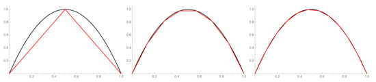
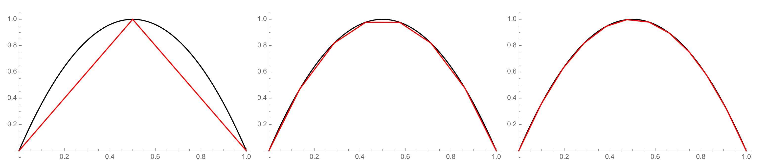
Let a function $f_1$, whose graph can be seen in Figure 2, be given. The chosen parameters are $\chi =0.69,{\mathsf{\Phi }}_1=2.45,{\mathsf{\Phi }}_2=1.65$, and the metric $d_1$ is used. In this example, $\ell =3,8,12$, $D=80$, and $I=100$. This function has two monotone parts, so the choice of the linear parts depends on the accuracy of what we want to obtain. In Figure 3, we can see the difference between $3,8$, and 12 points.

Figure 3. The graphs of the original function $f_1$ (the black line) and its piecewise linearizations $l_{f_1}$ (the red line), where $\ell =3,8,12$.

Example 4.

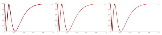
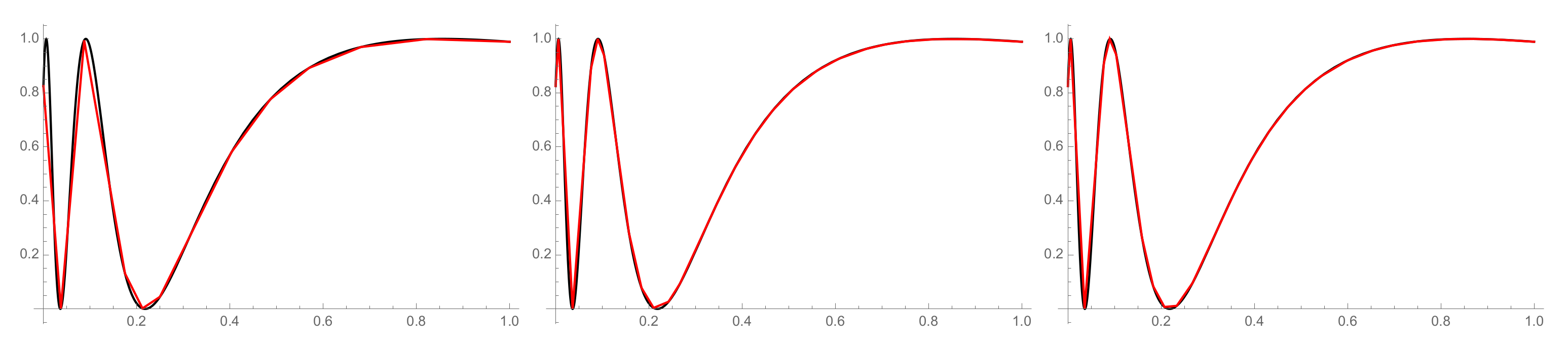
Let a function $f_2$, whose graph is depicted in Figure 2, be given. The initial parameters are $\chi =0.69,{\mathsf{\Phi }}_1=2.45,{\mathsf{\Phi }}_2=1.65$; the metric $d_1$ is chosen; $\ell =12$, $I=100$. As we can see, the first monotone parts are narrower, so if we choose $D=80$, the algorithm cannot approximate the first part correctly. For illustration, we take $D=500$ and $D=1000$ (see Figure 4).

Figure 4. The graphs of the original function $f_2$ (the black lines) and its piecewise linearizations $l_{f_2}$(the red lines), where $D=80,500,1000$.

Example 5.

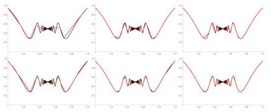
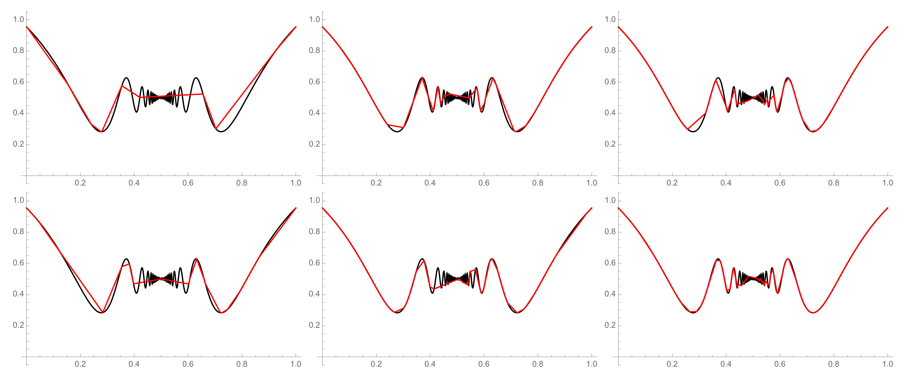
Let a function $f_5$ be given, and its graph can be seen in Figure 2. The initial parameters $\chi =0.69,{\mathsf{\Phi }}_1=2.45,{\mathsf{\Phi }}_2=1.65$ with the metric $d_1$ were chosen. In the first part of Figure 5, $\ell =12,40,100$, $I=100$, and $D=80$. In the second part of the figure, $\ell =25,60,100$, $I=100$, and $D=1000$.

Figure 5. The graphs of the original function $f_5$ (the black lines) and its piecewise linearizations $l_{f_5}$ (the red lines), where $\ell =12,40,100$, $I=100$, $D=80$ (the first row) and $\ell =25,60,100$, $I=100$, $D=1000$ (the second row).

We intentionally chose a function of this shape, namely with infinitely many pieces of monotonicity, and a simple observation confirmed that the problem can occur and the proposed solutions are unstable. The algorithm is not able to approximate all monotone parts correctly, and as we can see in Figure 5, the result need not always be as required. In this particular case, parameters D and ℓ should be much higher, and the calculation would take a bit more time.

The latter example brings us to the discussion on the complexity of the proposed algorithm.

3.5. Complexity of the Proposed Algorithm

In this subsection, we provide the computational complexity with the Big O notation, and we also show the computation time of the linearization process of the functions introduced in Section 3.2.

3.5.1. Computational Complexity

Let n be the input data size. The input data preprocessing of this algorithm has a computational complexity equal to $n^2$; the main loop has a computational complexity equal to $n^3$; the complexity of the last algorithm part, mainly consisting of drawing graphs, is equal to $n^2$; thus, the final complexity is given by the sum of all parts $n^2+n^3+n^2$. The Big O notation of this algorithm is $O\left(n^3\right)$.

3.5.2. Computation Time

Computation time is significantly influenced by more factors, especially the number of linear parts ℓ, iterations I, discretization points D, and also, the machine used for compiling. In Table 7, we can see the time dependent on ℓ and D, which are the most important values for the algorithm’s accuracy. The test was executed on the functions introduced in Section 3.2 with random parameters $\chi =0.69,{\mathsf{\Phi }}_1=2.45$, ${\mathsf{\Phi }}_2=1.65$, the metric $d_1$, $I=100$, and $n=25$.

Table 7. Computing time in seconds.

		$D=80$	$D=200$	$D=500$	$D=1000$
$f_1$	$\ell =12$	1.232	1.408	1.951	2.719
	$\ell =18$	1.677	1.876	2.417	3.187
	$\ell =25$	2.212	2.361	2.989	3.779
	$\ell =50$	3.881	4.172	4.993	5.843
$f_2$	$\ell =12$	1.357	1.515	2.058	2.869
	$\ell =18$	1.793	1.998	2.562	3.414
	$\ell =25$	2.295	2.515	3.179	4.034
	$\ell =50$	3.953	4.445	5.539	6.256
$f_3$	$\ell =12$	1.628	1.832	2.429	3.208
	$\ell =18$	2.274	2.473	3.095	3.892
	$\ell =25$	2.975	3.225	3.917	4.755
	$\ell =50$	5.169	5.677	6.626	7.616
$f_4$	$\ell =12$	1.390	1.604	2.122	2.789
	$\ell =18$	1.911	2.147	2.689	3.392
	$\ell =25$	2.499	2.777	3.340	4.093
	$\ell =50$	4.357	4.898	5.650	6.559
$f_5$	$\ell =12$	1.342	1.519	2.083	2.894
	$\ell =18$	1.778	2.026	2.613	3.444
	$\ell =25$	2.335	2.576	3.209	4.076
	$\ell =50$	4.002	4.474	5.427	6.377

${}^a$ Compiled in Python 3.8 (CPU: AMD 2920X, RAM: 32 GB, GPU: AMD RX VEGA64).

4. Approximation of Fuzzy Dynamical Systems

In this section, we present a generalization of the algorithm originally introduced in [20]. In the first part, we briefly comment on the algorithm in order to make the second technical part more legible. To simplify the notation below, we considered $X=[0,1]$. However, our algorithm can be easily adapted to an arbitrarily closed nondegenerated subinterval of the real line $\mathbb{R}$.

The main idea of the following algorithm is to compute a trajectory of a given discrete fuzzy dynamical subsystem $(\mathbb{F}\left(X\right),z_f)$, which is a natural and unique extension of a discrete dynamical system $(X,f)$. The main idea behind the previous algorithm [20] was to calculate Zadeh’s extension with the help of calculations on smaller intervals, i.e., pieces of linearity of both the map f and the fuzzy set A. This allowed computing Zadeh’s extension on a limited number of points. To be able to generalize the previous algorithm, we need to find appropriate linearizations. For this reason, the PSO-based linearization introduced in Section 2 was used.

In Step 1, the PSO-based linearization proposed in the previous section is used to find an appropriate linearization of the function f (resp. of the fuzzy set A, but the latter case is usually not needed).

In Step 2, it is shown how to decompose $X=[0,1]$ into finitely many subintervals and what points should be chosen for the calculation of Zadeh’s extension. Instinctively, it is important (and mostly, also sufficient) to consider the turning points of the function f and the turning points of a given fuzzy set A. The union of all such turning points defines a set J from which the starting and ending points of each interval of the decomposition of $[0,1]$ are generated.

In Step 3, Zadeh’s extension on intervals given by properly chosen pairs $d_I,d_{I+1}$ of points is computed in order to define linear elements from which the image $z_f\left(A\right)$ is reconstructed. This is a partial outcome from which we obtain a finite set of linear functions, and by using pointwise maxima of such linear parts, we obtain a graph of the image $z_f\left(A\right)$ of the fuzzy set A.

The process that is described in Steps 2 and 3 is repeated until we obtain the chosen number M of iterations. Below, we demonstrate several trajectories of fuzzy initial states A in a given dynamical system $\left(\right[0,1],f)$, which represent the final results of the proposed algorithm, i.e., a 3D plot of all evaluated iterations $z_f\left(A\right)$, $z_f^2\left(A\right)$, …, $z_f^M\left(A\right)$.

4.1. Pseudocode

Now, a bit more formal description of the algorithm consisting of six steps follows:

• Initialization—let the following items be given:
  • A continuous function $f:[0,1]\to [0,1]$;
  • A piecewise linear fuzzy set $A:[0,1]\to [0,1]$, defined by points $(a_I,b_I)\in [0,1]\times [0,1]$, where $I=1,2,\cdots ,n$,
    $A\left(y\right)=\left\{\begin{array}{cc}{b}_1+(b_2-b_1)\frac{(y-a_1)}{(a_2-a_1)},\hfill & a_1\le y\le a_2,\hfill \\ b_2+(b_3-b_2)\frac{(y-a_2)}{(a_3-a_2)},\hfill & a_2\le y\le a_3,\hfill \\ ⋮\hfill \\ b_{n-1}+(b_n-b_{n-1})\frac{(y-a_{n-1})}{(a_n-a_{n-1})},\hfill & a_{n-1}\le y\le a_n;\hfill \end{array}\right.$
  • A number of iterations $M\in \mathbb{N}$. Let $k=1$;
• Step 1:
  • Use the PSO algorithm (see Section 2) to find a linearization $l_f$ of a function f, i.e., to find a sequence of pairs $({\mathbf{x}}^{k_1},f\left({\mathbf{x}}^{k_1}\right))$ giving an appropriate linearization of a function f. For our notion, let $({\mathbf{x}}^{k_1},f\left({\mathbf{x}}^{k_1}\right)):=(c_I,s_I)$, where $I=1,\cdots ,\ell$;
• Step 2:
  • Create a set J of s linear segments $L_I$ of $l_f$ obtained from linear segments of A by the following inductive procedure. Whenever $c_j\in (a_I,a_I^{\prime })$ for some $L_I^{\prime }:=L_I((a_I,b_I),(a_I^{\prime },b_I^{\prime }))\in J$ and m is the number of elements in J, then J obtains two new linear segments $L_I,L_{m+1}$ instead of $L_I^{\prime }$, where $L_I=((a_I,b_I),(c_j,A\left(c_j\right)))$ and $L_{m+1}=((c_j,A\left(c_j\right)),(a_I^{\prime },b_I^{\prime }))$. This step is used repeatedly (if needed) in an analogous way. This way, we obtain a finite set of s linear segments $L_I=((a_I,b_I),(a_I^{\prime },b_I^{\prime }))$ from J;
• Step 3:
  • For $I=1,2,\dots ,s$ and for every linear segment $L_I=((a_I,b_I),(a_I^{\prime },b_I^{\prime }))$ from J, we compute its image $z_{l_f}\left(L_I\right)$ under Zadeh’s extension of the map $l_f$ restricted to $[a_I,a_I^{\prime }]$. More precisely, for every $L_I$, we obtain a linear segment $z_{l_f}\left(L_I\right)=((l_f\left(a_I\right),b_I),(l_f\left(a_I^{\prime }\right),b_I^{\prime }))$;
  • Take pointwise maxima of the obtained linear segments of $z_{l_f}\left(L_I\right)$, $I=1,2,\cdots ,s$, in order to obtain the graph of $z_{l_f}^k\left(A\right)$;
• Step 4:
  • If $k=M$, then the algorithm is finished;
  • If $k<M$, then put $k=k+1$, and repeat the whole procedure, i.e., continue from Step 2;
• Output:
  • Depict images of $z_f\left(A\right),\cdots ,z_f^M\left(A\right)$ in a 3D plot.

4.2. Examples

In this subsection, the algorithm for the approximation of fuzzy dynamical systems is demonstrated with the help of three examples. Below, we take three interval maps $g_1$, $g_2$, and $g_3$ and an appropriate fuzzy set $A_I$, $I=1,2,3,$ as the initial stages, and then, we compute the first tens of iterations to demonstrate the time evolution of the given initial state.

Example 6.

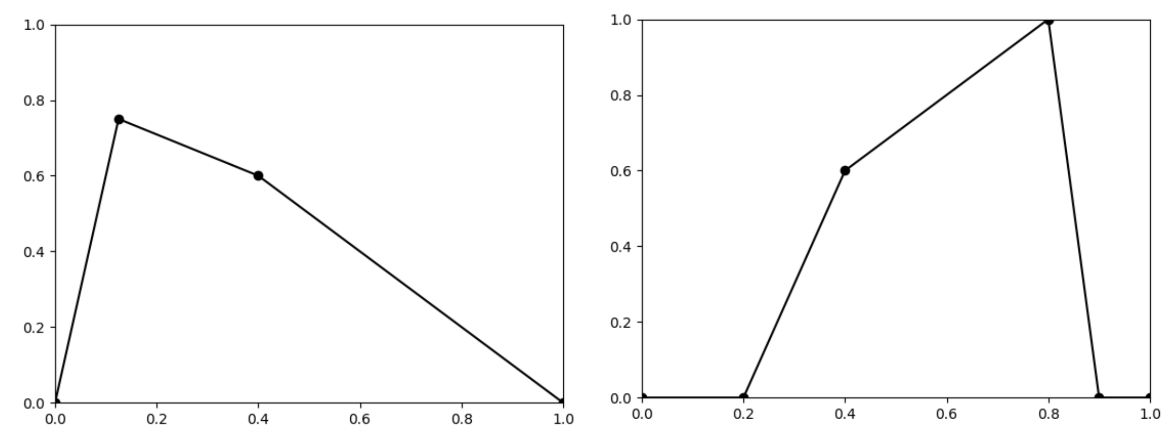
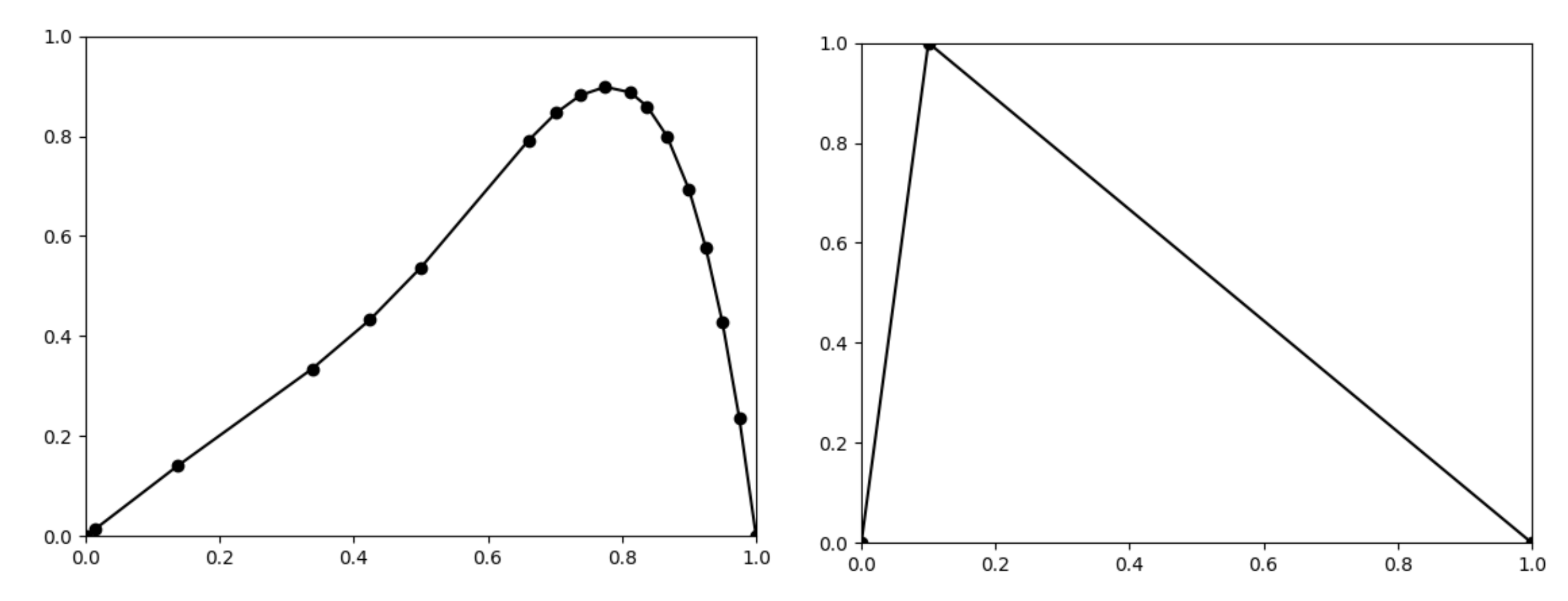
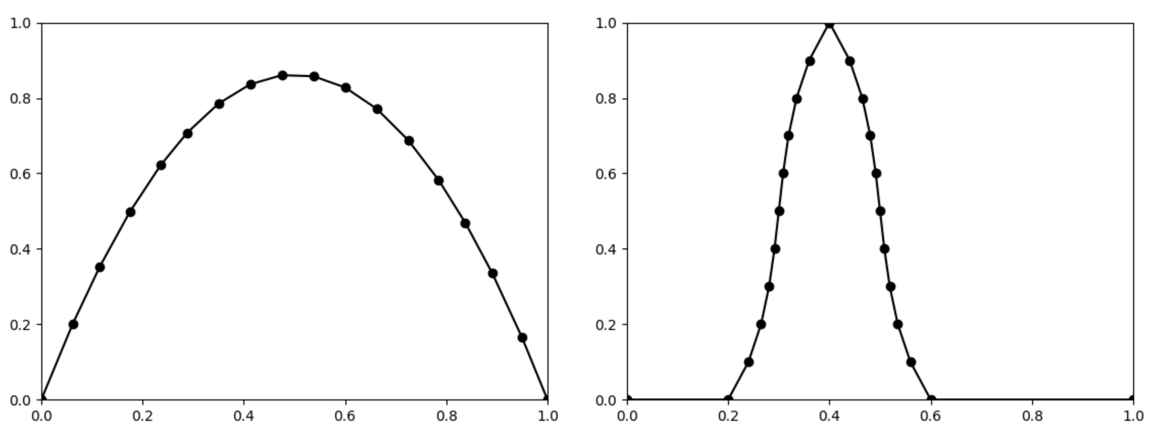
Let a piecewise linear function $g_1$ be given by five points $\left\{\right[0,0],[1/8,3/4],[2/5,3/5],[1,0\left]\right\}$, and let a piecewise linear fuzzy set $A_1$ be given by the following points $\left\{\right[0,0],[1/5,0],[2/5,3/5],[4/5,1],[9/10,0],[1,0\left]\right\}$ (see Figure 6).

Figure 6. The graphs of the function $g_1$ given by 4 points (left) and the fuzzy set $A_1$ given by 6 points (right).

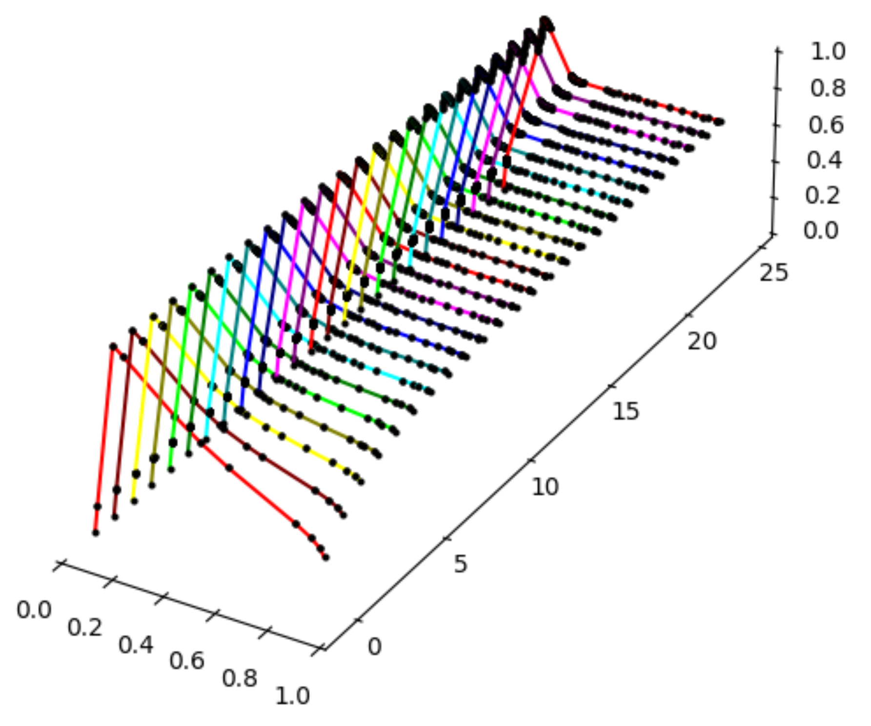
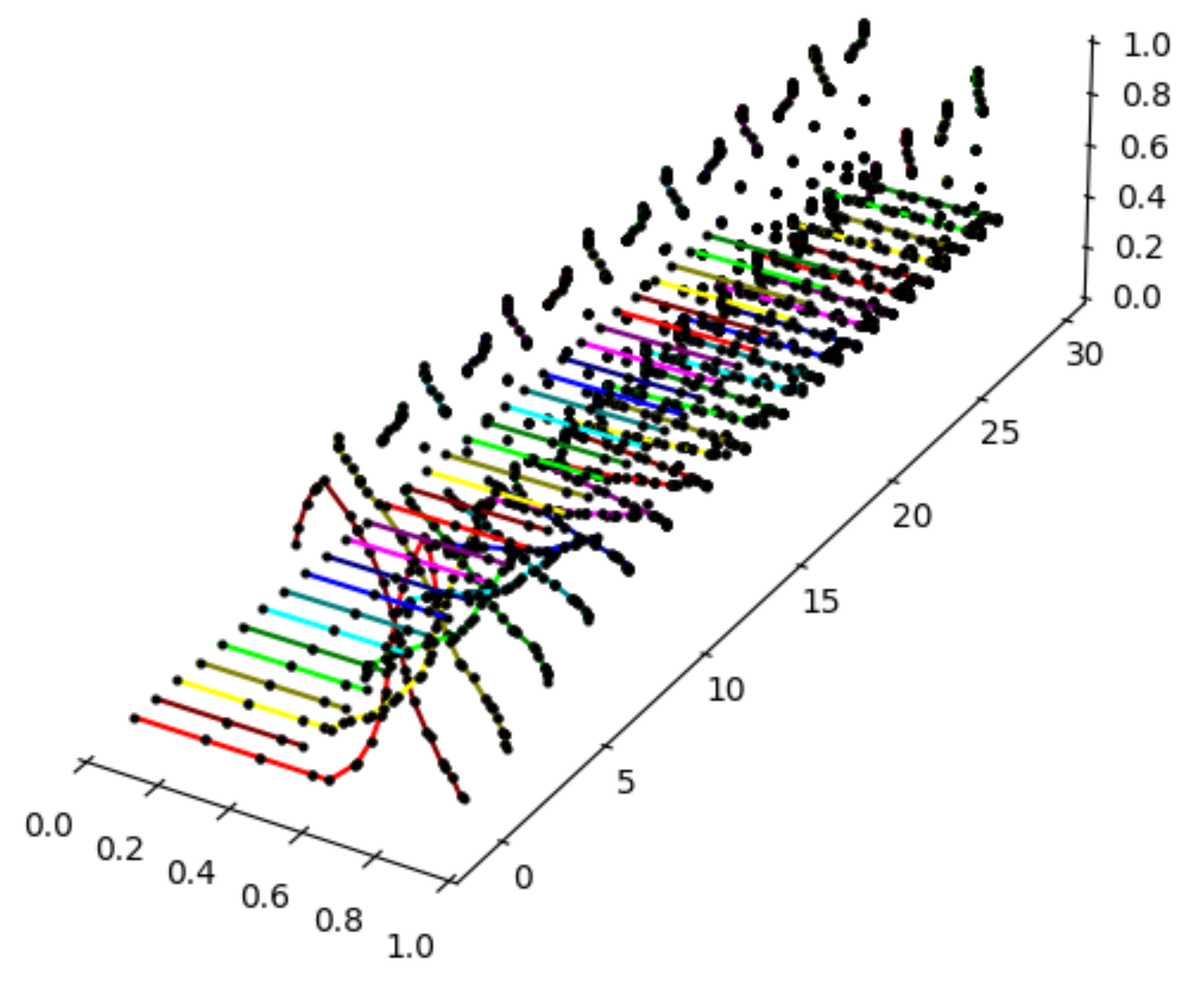
Now, we can use the algorithm introduced in Section 4. Below (see Figure 7), we can see a final plot that contains images of the fuzzy set $A_1$ for the first 30 iterations. This example gives a precise trajectory; the linearization of the function $g_1$ was not needed.

Figure 7. The graphs of $z_{{\tilde{g}}_1}\left(A_1\right),\cdots ,z_{{\tilde{g}}_1}^{30}\left(A_1\right)$.

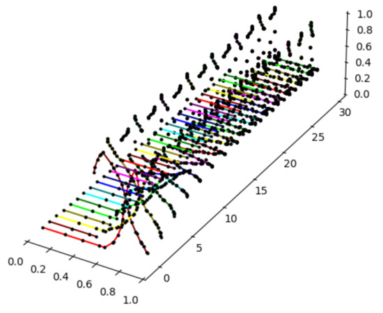
Example 7.

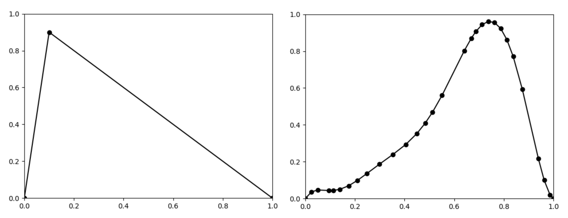
Let a piecewise linear function $g_2$ be given by a formula:

$$g_2\left(x\right)=(-2.9+(-4.1+(-15.6-14(-0.8+x))(-0.2+x))(-0.6+x))(-1+x)x$$

and let a piecewise linear fuzzy set $A_2$ be given by points $\left\{\right[0,0],[1/10,1],[1,0\left]\right\}.$ First, the PSO algorithm, which searches for a suitable linearization of a function $g_2$, is applied. Therefore, we have a linearized function $l_{g_2}$, with $\ell =17,D=80,I=100$, which can be seen in Figure 8. Then, the algorithm for the approximation of fuzzy dynamical system can continue.

Figure 8. The graphs of the linearized function $l_{g_2}$ given by 18 points (left) and the fuzzy set $A_2$ given by 3 points (right).

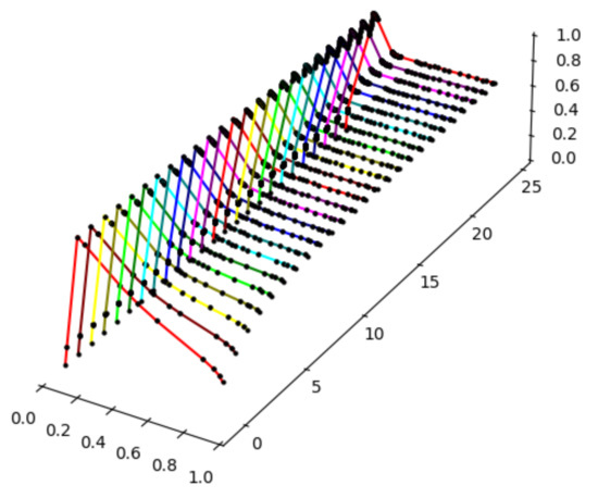
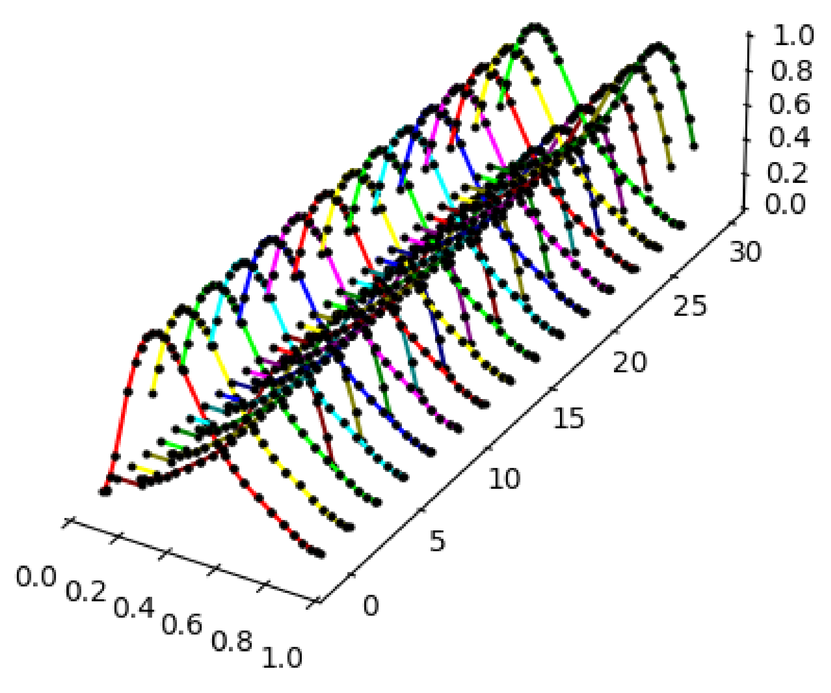
Finally, a plot containing the trajectory of the fuzzy set $A_2$ for the first 25 iterations can be seen (see Figure 9).

Figure 9. The graphs of $z_{l_{g_2}}\left(A_2\right),\cdots ,z_{l_{g_2}}^{25}\left(A_2\right)$.

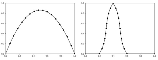
Example 8.

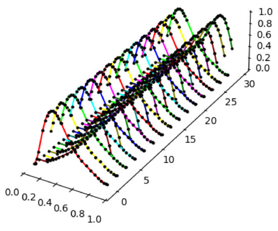
Let a piecewise linear function $g_3$ be given by three points $\left\{\right[0,0\left]\right\},[1/10,9/10],[1,0]\}$, and let $A_3$ be given by 30 points, as depicted in Figure 10. Now, we can use the algorithm for the approximation of the trajectory within an induced fuzzy dynamical system.

Figure 10. The graphs of the function $l_{g_3}$ given by 3 points (left) and the fuzzy set $A_3$ given by 30 points (right).

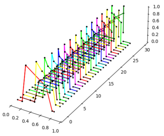
Again, a plot containing the first 30 elements of the trajectory of the fuzzy set $A_3$ under the map $z_{l_{g_3}}$ can be seen (see Figure 11). As we can see, the trajectory tends to have a periodic behavior.

Figure 11. The graphs of $z_{l_{g_3}}\left(A_3\right),\cdots ,z_{l_{g_3}}^{30}\left(A_3\right)$.

Example 9.

Let a function $g_4$ be given by the formula $g_4\left(x\right)=3.45x(1-x)$, and let a fuzzy set $A_4$ be given by 23 points (see Figure 12).

Figure 12. The graphs of the linearized function $l_{g_4}$ given by 18 points (left) and the fuzzy set $A_4$ given by 23 points (right).

To be able to calculate the approximation of Zadeh’s extension of $g_4$ we need to linearize the function $g_4$ first. Thus, we use the PSO algorithm to find the an appropriate linearization of the function $g_4$.

Below (Figure 13), we can see a final plot containing the first 30 iterations of the trajectory of the fuzzy set $A_4$ under the map $z_{l_{g_4}}$.

Figure 13. The graphs of $z_{l_{g_4}}\left(A_4\right),\cdots ,z_{l_{g_4}}^{30}\left(A_4\right)$.

4.3. Algorithmic Complexity of Approximations of Fuzzy Dynamical Systems

In this subsection, the computational complexity with the Big O notation and the computation time of a few examples are provided.

4.3.1. Computational Complexity

Let n be the input data size. The Big O notation of this algorithm is $O(n^{2}log\left(n\right))$. The input data preprocessing has a computational complexity equal to n; the main loop has a computational complexity equal to $n^{2}log\left(n\right)$; the last algorithm part has a complexity equal to $n^2$. Thus, the final complexity is $O(n^{2}log\left(n\right))$, which is given by the sum of all parts $n+n^{2}log\left(n\right)+n^2$.

4.3.2. Computation Time

In Table 8, we provide the computation time of the examples introduced in Section 4.2 for a rough orientation.

Table 8. Computing time in seconds.

	10 Iterations	100 Iterations	1000 Iterations	10,000 Iterations
Example 1	0.35	2.11	24.59	317.12
Example 2	2.12	158.42	17,457.49	over 5 h
Example 3	0.62	5.26	66.99	794.6
Example 4	2.83	147.44	16,552.96	over 5 h

${}^a$ Compiled in Python 3.8 (CPU: AMD 2920X, RAM: 32 GB, GPU: AMD RX VEGA64).

5. Accuracy of Approximations of Fuzzy Dynamical Systems

It is indisputable that the accuracy of approximations of fuzzy dynamical systems largely depends on the given input values and also the parameter selection. Generally, known as a butterfly effect [27] in dynamical systems, a small change of the side of inputs can cause a large change in the output, especially in long-term observations. In the previous version of our algorithm [20], we dealt with calculations of piecewise linear functions and fuzzy sets, so there was no need to open any discussion on accuracy. However, because the functions (and fuzzy sets) need not always be piecewise linear, there is a natural demand for the algorithm proposed in this paper. Since PSO is a stochastic algorithm based on computing with random parameters, various linearizations provided by the PSO algorithm can give us similar, close to each other, but different outputs. Consequently, there will definitely be different trajectories that will differ from each other especially in higher iterations. However, it is natural to ask how significant the influence of these small changes for the algorithm used for the computations of trajectories of an induced fuzzy dynamical system is.

To provide a discussion on this topic, we considered tens of iterations only. Concerning the butterfly effect mentioned above, it is natural that, in general, no approximation prepared at the very beginning can be sufficient in long-term behavior, and in particular applications, some form of recalculations and adjustments will be needed, which is supposed to be a part of our future work. Consequently, to show some observations on the stability of the proposed algorithm, we prepared a comparison of the beginning of the trajectories. For this comparison, we prepared yet another algorithm called a testing algorithm below, which is based on direct calculations of a huge number of points of the phase space and their subsequent reduction. Therefore, we considered it as a perspective for long-term estimates; however, we considered it suitable for our purposes because it provides exact values of Zadeh’s extension when used with a big number of points. The calculation of the distances in the tables below was performed with the help of the Euclidean and Manhattan metrics.

Comparison

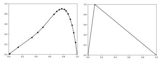
To demonstrate the stability, we chose Example 7 from Section 4.2. Let the function $g_2$ be given by the following formula (see Figure 14):

$$g_2\left(x\right)=-2.9+(-4.1+(-15.6-14(-0.8+x))(-0.2+x))(-0.6+x))(-1+x)x.$$

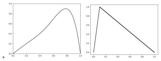
Figure 14. The graph of the function $g_2$ (left) and a fuzzy set A represented by 2020 equidistantly distributed points (right).

In Figure 15, one can see the results calculated with the help of the testing algorithm on the right side, and the second example (on the left side) is given by the algorithm based on the PSO linearization (proposed in Section 4).

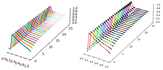
Figure 15. The graphs of $z_{l_{g_2}}\left(A\right),\cdots ,z_{l_{g_2}}^{25}\left(A\right)$.

Upon the first sight, we can see that the trajectories are similar. To be more specific about how stable the proposed algorithm is, we calculated the distances between each iteration with the Euclidean and Manhattan distances introduced in Section 1.6 (see Table 9 and Table 10).

Table 9. The distances (Euclidean, Manhattan) between the testing algorithm and the proposed algorithm for $\ell =17$.

	Run 1	Run 2	Run 3	Run 4	Run 5
1.it	0.8919, 5.1155	1.566, 11.4928	1.5653, 11.4085	1.5659, 11.5735	1.0103, 7.0495
2.it	1.0983, 5.7121	1.963, 12.2853	1.9607, 12.1007	1.9627, 12.4276	1.2682, 7.6393
3.it	1.0682, 5.6671	1.8581, 10.3098	1.8528, 10.0456	1.8575, 10.5338	1.2167, 7.2449
4.it	1.0705, 6.207	1.697, 9.2699	1.7696, 9.4782	1.6962, 9.5903	1.2425, 7.7789
5.it	0.9993, 6.6038	1.5301, 8.7346	1.5138, 8.3465	1.5295, 9.1549	1.0583, 7.59
6.it	0.8675, 6.8625	1.3713, 8.5283	1.3462, 8.0865	1.3712, 9.0421	0.946, 7.9534
7.it	0.6659, 7.0358	1.2889, 8.7891	1.2542, 8.3194	1.2901, 9.4107	0.9829, 8.7625
8.it	0.6933, 7.7999	1.1768, 8.9707	1.1293, 8.5039	1.1801, 9.7274	1.0224, 9.688
9.it	0.7192, 8.5805	1.0354, 9.0945	0.9697, 8.6472	1.0425, 9.9978	0.8383, 9.8451
10.it	0.7436, 9.3818	1.2491, 10.4618	1.1856, 10.0458	1.2586, 11.5175	1.0863, 11.389
11.it	0.7678, 10.1832	1.1043, 10.5292	1.0207, 10.1579	1.12, 11.741	0.9025, 11.5197
12.it	0.7914, 10.9849	1.1364, 11.2221	1.0444, 10.9133	1.1576, 12.5993	0.9294, 12.2951
13.it	0.815, 11.7803	0.9626, 11.235	0.8387, 11.0108	0.9958, 12.793	0.9661, 13.2032
14.it	0.8383, 12.5751	0.9962, 11.8828	0.8642, 11.7657	1.0374, 13.6378	0.9929, 13.9848
15.it	0.8614, 13.3641	1.0289, 12.5086	0.8896, 12.523	1.0789, 14.4797	1.0293, 14.9047
16.it	0.8844, 14.1493	1.0606, 13.1153	0.9146, 13.2817	1.12, 15.3187	1.0557, 15.6904
17.it	0.609, 14.2639	1.0917, 13.7037	0.9395, 14.0371	1.161, 16.1522	0.8597, 15.9405
18.it	0.6414, 15.0579	1.1216, 14.2828	0.9633, 14.7924	1.201, 16.9827	0.8908, 16.7227
19.it	0.674, 15.8522	0.9309, 14.1761	0.718, 14.8648	1.0399, 17.1336	0.9214, 17.4992
20.it	0.707, 16.6491	1.1796, 15.4016	1.0094, 16.2746	1.2798, 18.6267	0.9629, 18.4067
21.it	0.7403, 17.4479	0.9981, 15.2692	0.7761, 16.3257	1.1295, 18.7622	0.9914, 19.1622
22.it	0.7744, 18.2657	1.0302, 15.8061	0.8041, 17.0482	1.1724, 19.5691	1.0305, 20.0508
23.it	0.8092, 19.0897	1.0613, 16.3339	0.8318, 17.7678	1.214, 20.3694	1.0567, 20.7841
24.it	0.8448, 19.9349	1.2875, 17.5359	1.0976, 19.1672	1.428, 21.8433	1.094, 21.6593
25.it	0.881, 20.7703	1.1208, 17.3695	0.8869, 19.2024	1.2929, 21.9435	1.1189, 22.3747

Table 10. The distances (Euclidean, Manhattan) between the testing algorithm and the proposed algorithm for $\ell =25$.

	Run 1	Run 2	Run 3	Run 4	Run 5
1.it	1.5642, 10.4592	0.8908, 4.2392	0.8912, 4.4135	1.2241, 6.9286	0.9287, 4.7612
2.it	1.9588, 10.7188	1.1626, 4.6363	1.0964, 4.439	1.5573, 7.3061	1.1633, 4.6546
3.it	1.8489, 8.2665	1.0623, 3.7226	1.0645, 3.9701	1.5058, 6.0132	1.1641, 4.0716
4.it	1.6798, 6.6697	1.0606, 3.7612	1.0644, 4.0904	1.4042, 5.246	1.0603, 3.5433
5.it	1.5013, 5.6034	0.9832, 3.6547	0.9895, 4.0835	1.2691, 4.6698	0.9827, 3.3467
6.it	1.3264, 4.8673	0.8415, 3.4435	0.8517, 3.9723	1.1876, 4.5088	0.8405, 3.0633
7.it	1.2255, 4.625	0.62, 3.1822	0.638, 3.8011	0.8711, 3.6628	0.8685, 3.3129
8.it	1.0879, 4.3399	0.6365, 3.509	0.6584, 4.2093	0.8929, 3.9885	0.8895, 3.5422
9.it	0.9088, 4.0241	0.6506, 3.8275	0.6763, 4.6053	0.911, 4.3057	0.6472, 3.1277
10.it	1.1254, 4.9738	0.6623, 4.1451	0.6918, 4.9916	0.9254, 4.6219	0.9201, 3.9785
11.it	0.9359, 4.6423	0.6733, 4.4663	0.7063, 5.3718	0.6763, 4.293	0.6675, 3.5389
12.it	0.9466, 4.9566	0.6833, 4.7987	0.7194, 5.7473	0.9495, 5.2703	0.6757, 3.7362
13.it	0.6915, 4.6111	0.6934, 5.14	0.732, 6.1185	0.6961, 4.9436	0.6834, 3.9269
14.it	0.6998, 4.9198	0.703, 5.4966	0.7438, 6.4878	0.7053, 5.279	0.6902, 4.113
15.it	0.7077, 5.2263	0.7127, 5.8664	0.7552, 6.8555	0.7145, 5.6215	0.6967, 4.2953
16.it	0.7152, 5.5327	0.7227, 6.249	0.7662, 7.2239	0.7237, 5.9727	0.7027, 4.4741
17.it	0.7229, 5.8398	0.2902, 5.9704	0.3886, 6.9216	0.2908, 5.6591	0.2213, 3.9769
18.it	0.7298, 6.1526	0.3115, 6.3742	0.4062, 7.293	0.31, 6.0275	0.2324, 4.1478
19.it	0.2921, 5.7953	0.3333, 6.786	0.4234, 7.6654	0.3297, 6.4022	0.2433, 4.3126
20.it	0.7446, 6.7901	0.355, 7.2022	0.4405, 8.0383	0.3498, 6.7842	0.2541, 4.4726
21.it	0.3219, 6.4371	0.3769, 7.6243	0.4572, 8.4119	0.3702, 7.1717	0.2648, 4.6297
22.it	0.3371, 6.7674	0.3986, 8.0527	0.4737, 8.7869	0.3909, 7.5698	0.2754, 4.7885
23.it	0.3525, 7.1021	0.42, 8.4847	0.4898, 9.1612	0.4117, 7.9721	0.286, 4.9452
24.it	0.7756, 8.1237	0.4408, 8.9201	0.5057, 9.5373	0.4325, 8.3832	0.2966, 5.1046
25.it	0.3834, 7.7849	0.4611, 9.3534	0.5215, 9.9133	0.453, 8.7923	0.3071, 5.2582

In Table 11, we provide five runs of the proposed algorithm, and for each of them, we calculated the distances to the elements of the trajectory of A provided by the testing algorithm and the PSO-based one; we demonstrate that they tend to provide a stable solution. The distances were calculated on a moving set of points given by images of 2020 points approximating A with their careful pruning lowering the number of approximating points. This tends to show a more practical behavior of the trajectory. In Table 12, we provide another comparison in which the pruned points are refilled by equidistantly distributed points. That calculation provided outcomes closer to the endograph distance, which showed a behavior closer to theoretical studies, e.g., in [3,28], and that is also why the butterfly effect is more observable in the latter case.

Table 11. The distances (Euclidean, Manhattan) between the testing and the proposed algorithm for $\ell =40$.

	Run 1	Run 2	Run 3	Run 4	Run 5
1.it	0.9581, 4.164	0.9245, 3.9838	0.8896, 3.6624	0.8553, 3.8953	0.9259, 4.2064
2.it	1.1620, 4.0212	1.1621, 4.2027	1.0947, 3.7035	1.0997, 4.7368	1.1634, 4.3623
3.it	1.1632, 3.4836	1.1635, 3.7722	1.0614, 3.1262	1.0727, 4.6947	1.1658, 3.9224
4.it	1.0589, 2.8857	1.0597, 3.2758	1.0591, 3.0348	1.0787, 5.1298	1.0640, 3.4514
5.it	0.9805, 2.5967	0.9817, 3.0868	0.9807, 2.7742	1.0128, 5.3904	0.9889, 3.3021
6.it	0.8370, 2.2123	0.8391, 2.8005	0.8374, 2.4034	0.8895, 5.5319	0.8510, 3.0571
7.it	0.8641, 2.3681	0.6158, 2.4489	0.6127, 1.9762	0.7034, 5.6009	0.6374, 2.7494
8.it	0.8841, 2.5122	0.8876, 3.2974	0.6273, 2.1294	0.7386, 6.2316	0.9069, 3.6503
9.it	0.6381, 2.0106	0.6442, 2.8962	0.6392, 2.2797	0.7720, 6.8422	0.6769, 3.2981
10.it	0.9124, 2.7679	0.9177, 3.7655	0.6484, 2.4325	0.8035, 7.4366	0.9459, 4.2058
11.it	0.6547, 2.2352	0.6638, 3.3555	0.6566, 2.582	0.8343, 8.0102	0.7092, 3.8233
12.it	0.6609, 2.344	0.6717, 3.5941	0.6631, 2.7297	0.5626, 7.9099	0.7239, 4.0827
13.it	0.6665, 2.4516	0.6792, 3.8382	0.6692, 2.8766	0.8928, 9.0961	0.7384, 4.3415
14.it	0.6711, 2.5577	0.6859, 4.0917	0.6743, 3.0270	0.9207, 9.6089	0.7522, 4.5992
15.it	0.6751, 2.662	0.6924, 4.3556	0.6789, 3.1821	0.9479, 10.105	0.7659, 4.8562
16.it	0.6786, 2.7652	0.6987, 4.6295	0.6832, 3.3433	0.7070, 9.9192	0.7793, 5.1142
17.it	0.1092, 2.1953	0.2101, 4.2436	0.1389, 2.8395	0.7402, 10.3864	0.4188, 4.7006
18.it	0.1143, 2.2967	0.2244, 4.54	0.1475, 3.0161	0.7725, 10.8465	0.4403, 4.9594
19.it	0.1193, 2.3959	0.2394, 4.8484	0.1563, 3.199	0.8038, 11.298	0.4615, 5.2186
20.it	0.1243, 2.4913	0.2550, 5.1663	0.1653, 3.3876	0.8343, 11.7414	0.4824, 5.4763
21.it	0.1291, 2.5846	0.2711, 5.4949	0.1747, 3.584	0.8639, 12.1762	0.5029, 5.7325
22.it	0.1340, 2.6804	0.2876, 5.8357	0.1845, 3.7945	0.8927, 12.6057	0.5231, 5.9887
23.it	0.1390, 2.7771	0.3044, 6.1845	0.1948, 4.0166	0.9208, 13.0294	0.5430, 6.2452
24.it	0.1442, 2.8775	0.3215, 6.5434	0.2057, 4.2559	0.9482, 13.447	0.5627, 6.5046
25.it	0.1496, 2.978	0.3388, 6.908	0.2171, 4.5056	0.9747, 13.8553	0.5820, 6.7657

Table 12. The distances (Euclidean, Manhattan) between the testing and the proposed algorithm in 2020 points for $\ell =40$.

	Run 1	Run 2	Run 3	Run 4	Run 5
1.it	0.9581, 4.164	1.5653, 11.4085	0.8896, 3.6624	0.8553, 3.8953	0.9259, 4.2064
2.it	1.1621, 4.1663	1.9612, 12.7846	1.0948, 3.8907	1.1009, 5.1424	1.1637, 4.5722
3.it	1.1633, 3.8174	1.9757, 12.4359	1.0616, 3.5694	1.0773, 5.6598	1.1670, 4.4189
4.it	1.1843, 3.9087	2.2011, 14.8196	1.1847, 4.283	1.2092, 7.105	1.1906, 4.6808
5.it	0.9811, 3.3538	1.7223, 12.8369	0.9817, 3.7878	1.0309, 7.7422	0.9933, 4.344
6.it	0.8382, 3.2151	1.6008, 13.6743	0.8392, 3.7529	0.9272, 8.9988	0.8616, 4.605
7.it	0.8655, 3.5041	1.8712, 16.5554	0.6156, 3.4628	0.7572, 9.2505	0.6533, 4.349
8.it	0.8860, 3.9035	1.7092, 17.2633	0.6315, 3.995	0.8170, 10.8973	0.9245, 5.7198
9.it	0.9021, 4.2084	1.6292, 18.1477	0.9043, 5.0636	1.0604, 12.2797	0.9445, 5.9602
10.it	0.9151, 4.4996	2.2977, 23.9888	0.6544, 4.8894	0.9081, 13.3456	0.9678, 6.5753
11.it	0.6597, 4.2437	1.7037, 21.5917	0.6647, 5.5777	0.9572, 14.6087	0.7493, 6.578
12.it	0.6669, 4.6091	1.6183, 23.3675	0.6721, 5.9713	0.7850, 15.9054	0.7757, 7.2886
13.it	0.9431, 5.5407	1.6391, 24.0636	0.9479, 7.1016	1.2524, 18.1113	1.0361, 8.5428
14.it	1.1587, 6.4636	1.7918, 25.41	1.1638, 8.2782	1.0868, 17.6525	1.2395, 9.4029
15.it	1.3438, 7.6741	1.8359, 27.9844	1.1716, 8.7462	1.4963, 21.4299	1.4260, 10.8137
16.it	0.6890, 6.0338	1.2867, 26.1661	0.6994, 7.8038	1.0118, 20.3395	0.8798, 10.0349
17.it	0.1612, 5.5331	1.1384, 26.785	0.2044, 7.3743	1.0329, 20.8362	0.5516, 8.8711
18.it	0.1703, 5.8584	1.7918, 30.7683	0.2178, 7.8088	1.0420, 20.8536	0.5699, 9.0907
19.it	0.1775, 6.0815	0.9871, 28.0267	0.2277, 8.1142	1.1324, 22.483	0.6296, 10.1419
20.it	0.1858, 6.3469	1.2572, 30.9921	0.2345, 8.3376	1.2104, 24.2562	0.6629, 10.7395
21.it	0.1914, 6.5616	1.0957, 31.7035	0.2480, 8.7462	1.2284, 24.8786	0.6771, 10.793
22.it	0.2033, 6.8999	1.1531, 33.7333	0.2534, 8.9109	1.2858, 26.0793	0.7062, 11.3334
23.it	0.2064, 7.028	1.1959, 35.0461	0.2753, 9.4986	1.3534, 27.889	0.7339, 12.113
24.it	0.2137, 7.1825	1.4009, 36.7751	0.2740, 9.4073	1.3634, 27.4815	0.7737, 12.2315
25.it	0.2184, 7.3571	1.2388, 37.0353	0.2984, 10.0981	1.4508, 29.8616	0.7946, 12.9525

First of all, the next tables show the dependence of the choice on the number of linear parts, i.e., when $\ell =17,25$, and 40, respectively.

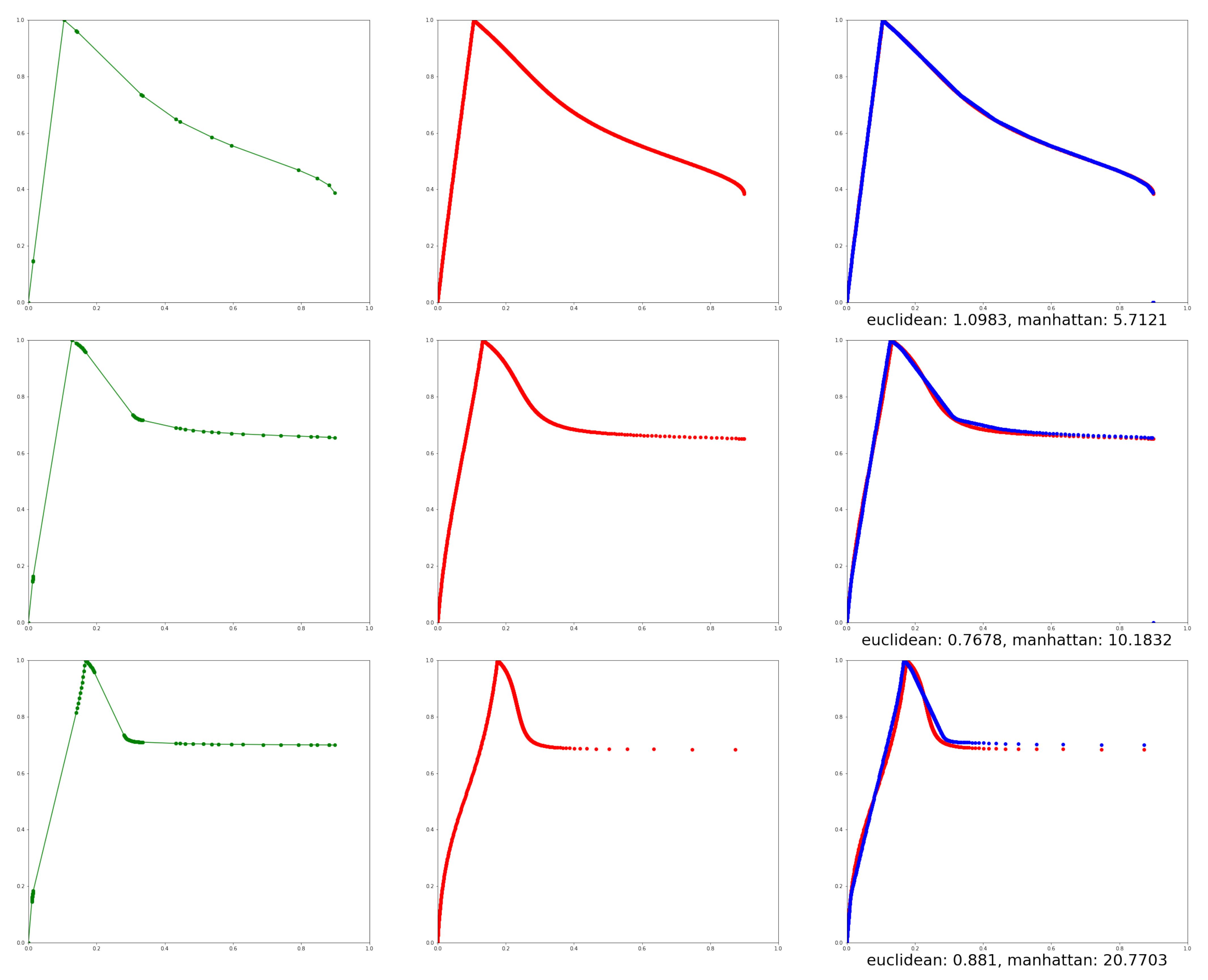
In Figure 16, we also depict the first, tenth, and twenty-fifth iteration. The green trajectory is the result of our proposed algorithm, the red trajectory is the result given by the testing algorithm, while the last image illustrates the difference between the selected iterations.

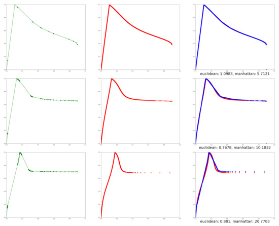
Figure 16. Accuracy of the algorithm—the 1st, 10th, and 25th iteration.

6. Conclusions

In this contribution, we introduced an algorithm that can be used for simulations of fuzzy dynamical systems induced by one-dimensional maps. The proposed algorithm is partially based on the calculation of Zadeh’s extension on smaller linear pieces implemented in a previous paper ([20]). The latter approach covered topologically large, yet not the full class of continuous interval maps. To be able to compute it for any arbitrary continuous interval map, we focused on the linearization process and adapted the PSO algorithm to search for a suitable linearization of a given map. This approach provides us an approximated trajectory of the initial state A in a general one-dimensional fuzzy dynamical system. To highlight some advantages in contrast to previous approaches, we are not restricted to fuzzy numbers only (the family of fuzzy sets is far richer), we are not restricted to convex fuzzy sets (convexity is not preserved by higher iterations), and, if needed, we are able to deal with discontinuous fuzzy sets (which naturally appear in higher iterations). We are also convinced that our approach will be generalized to higher dimensions, which would be a case not provided by previous approaches.

The proposed algorithm has been tested from several points of view. In the first part of the algorithm, the parameter selection in the PSO algorithm has been elaborated and, also, the algorithm complexity was discussed. The algorithm complexity was discussed also for the main part of the proposed algorithm and, subsequently, some trajectories of fuzzy dynamical systems derived by Zadeh’s extension were presented and briefly compared in precision. The next natural steps are to extend this algorithm into higher dimensions, to implement advanced features like automatic detection of pieces of linearity of the approximating map, to show implementations in particular applications and so on.

References

- Esmi, E.; Sussner, P.; Ignácio, G.B.D.; de Barros, L.C. A parametrized sum of fuzzy numbers with applications to fuzzy initial value problems. Fuzzy Sets Syst. 2018, 331, 85–104. [Google Scholar] [CrossRef]
- Pedro, F.S.; de Barros, L.C.; Esmi, E. Population growth model via interactive fuzzy differential equation. Inf. Sci. 2019, 481, 160–173. [Google Scholar] [CrossRef]
- Kupka, J. On fuzzifications of discrete dynamical systems. Inf. Sci. 2011, 181, 2858–2872. [Google Scholar] [CrossRef]
- Zhao, Y.; Cheng, W.-C.; Ho, C.-C. On sequential entropy of fuzzy systems. J. Intell. Fuzzy Syst. 2011, 34, 2021–2029. [Google Scholar] [CrossRef]
- Chalco-Cano, Y.; Misukoshi, M.T.; Román-Flores, H.; Flores-Franulic, A. Spline approximation for Zadeh’s extensions. Int. J. Uncertain. Fuzziness Knowl.-Based Syst. 2009, 7, 269–280. [Google Scholar] [CrossRef]
- Chalco-Cano, Y.; Román-Flores, H.; Rojas-Medar, M.; Saavedra, O.; Jiménez-Gamero, M.-D. The extension principle and a decomposition of fuzzy sets. Inf. Sci. 2007, 177, 5394–5403. [Google Scholar] [CrossRef]
- Scheerlinck, K.; Vernieuwe, H.; Baets, B.D. Zadeh’s extension principle for continuous functions of non-interactive variables: A parallel optimization approach. IEEE Trans. Fuzzy Syst. 2011, 20, 96–108. [Google Scholar] [CrossRef]
- Ahmad, M.Z.; Hasan, M.K. A new approach for computing Zadeh’s extension principle. Matematika 2010, 26, 71–81. [Google Scholar]
- Stefanini, L.; Sorini, L.; Guerra, M.L. Simulation of fuzzy dynamical systems using the LU-representation of fuzzy numbers. Chaos Solitons Fractals 2006, 29, 638–652. [Google Scholar] [CrossRef]
- Guerra, M.L.; Stefanini, L. Approximate fuzzy arithmetic operations using monotonic interpolations. Fuzzy Sets Syst. 2005, 150, 5–33. [Google Scholar] [CrossRef]
- Kupka, J. On approximations of Zadeh’s extension principle. Fuzzy Sets Syst. 2016, 283, 26–39. [Google Scholar] [CrossRef]
- Hanss, M. The transformation method for the simulation and analysis of systems with uncertain parameters. Fuzzy Sets Syst. 2002, 130, 277–289. [Google Scholar] [CrossRef]
- Otto, K.N.; Lewis, A.D.; Antonsson, E.K. Approximating α-cuts with the vertex method. Fuzzy Sets Syst. 1993, 55, 43–50. [Google Scholar] [CrossRef]
- Sánchez, D.E.; Wasques, V.F.; Arenas, J.P.; Esmi, E.; de Barros, L.C. On interactive fuzzy solutions for mechanical vibration problems. Appl. Math. Model. 2021, 96, 304–314. [Google Scholar] [CrossRef]
- Wasques, V.F.; Esmi, E.; Barros, L.C. Solution to the advection equation with fuzzy initial condition via sup-j extension principle. In Proceedings of the 19th World Congress of the International Fuzzy Systems Association (IFSA), 12th Conference of the European Society for Fuzzy Logic and Technology (EUSFLAT), and 11th International Summer School on Aggregation Operators (AGOP), Bratislava, Slovakia, 19–24 September 2021; Atlantis Press: Paris, France, 2021; pp. 134–141. [Google Scholar]
- Wasques, V.F.; Esmi, E.; Barros, L.C.; Sussner, P. The generalized fuzzy derivative is interactive. Inf. Sci. 2020, 519, 93–109. [Google Scholar] [CrossRef]
- Jardón, D.; Sánchez, I.; Sanchis, M. Transitivity in fuzzy hyperspaces. Mathematics 2020, 8, 1862. [Google Scholar] [CrossRef]
- Khatua, D.; Maity, K. Stability of fuzzy dynamical systems based on quasi-level-wise system. J. Intell. Fuzzy Syst. 2017, 33, 3515–3528. [Google Scholar] [CrossRef]
- Ma, C.; Zhu, P.; Lu, T. Some chaotic properties of fuzzified dynamical systems. SpringerPlus 2016, 5, 1–7. [Google Scholar] [CrossRef] [Green Version]
- Kupka, J.; Škorupová, N. Calculations of Zadeh’s extension of piecewise linear functions. In International Fuzzy Systems Association World Congress; Springer: Berlin/Heidelberg, Germany, 2019; pp. 613–624. [Google Scholar] [CrossRef]
- Kupka, J.; Škorupová, N. On PSO-based approximation of Zadeh’s extension principle. In International Conference on Information Processing and Management of Uncertainty in Knowledge-Based Systems; Springer: Berlin/Heidelberg, Germany, 2020; pp. 267–280. [Google Scholar] [CrossRef]
- Block, L.S.; Coppel, W.A. Dynamics in One Dimension; Springer: Berlin/Heidelberg, Germany, 2006. [Google Scholar] [CrossRef]
- Zadeh, L.A. Fuzzy sets. Inf. Control. 1965, 8, 338–353. [Google Scholar] [CrossRef] [Green Version]
- Kloeden, P. Fuzzy dynamical systems. Fuzzy Sets Syst. 1982, 7, 275–296. [Google Scholar] [CrossRef]
- Kennedy, J. Particle Swarm Optimization. In Encyclopedia of Machine Learning; Sammut, C., Webb, G.I., Eds.; Springer: Boston, MA, USA, 2011; pp. 760–766. [Google Scholar]
- Eberhart, R.; Kennedy, J. Particle swarm optimization. In Proceedings of the ICNN’95—International Conference on Neural Networks, Perth, Australia, 27 November–1 December 1995; Volume 4, pp. 1942–1948. [Google Scholar]
- D’Aniello, E.; Steele, T.H. Asymptotically stable sets and the stability of omega-limit sets. J. Math. Anal. Appl. 2006, 321, 867–879. [Google Scholar] [CrossRef] [Green Version]
- Canovás, J.; Kupka, J. On the topological entropy on the space of fuzzy numbers. Fuzzy Sets Syst. 2014, 257, 132–145. [Google Scholar] [CrossRef]
Publisher’s Note: MDPI stays neutral with regard to jurisdictional claims in published maps and institutional affiliations. |
© 2021 by the authors. Licensee MDPI, Basel, Switzerland. This article is an open access article distributed under the terms and conditions of the Creative Commons Attribution (CC BY) license (https://creativecommons.org/licenses/by/4.0/).