Article

A Map of the Poor or a Poor Map?

1
Poverty and Equity Global Practice, The World Bank Group, Washington, DC 98104, USA
2
Development Economics Data Group, The World Bank Group, Washington, DC 98104, USA
3
Department of Statistics, Universidad Carlos III de Madrid, 28903 Madrid, Spain
*
Author to whom correspondence should be addressed.
Mathematics 2021, 9(21), 2780; https://doi.org/10.3390/math9212780
Submission received: 28 September 2021 / Revised: 22 October 2021 / Accepted: 25 October 2021 / Published: 2 November 2021

Abstract

:
This paper evaluates the performance of different small area estimation methods using model and design-based simulation experiments. Design-based simulation experiments are carried out using the Mexican Intra Censal survey as a census of roughly 3.9 million households from which 500 samples are drawn using a two-stage selection procedure similar to that of Living Standards Measurement Study (LSMS) surveys. The estimation methods considered are that of Elbers, Lanjouw and Lanjouw (2003), the empirical best predictor of Molina and Rao (2010), the twofold nested error extension presented by Marhuenda et al. (2017), and finally an adaptation, presented by Nguyen (2012), that combines unit and area level information, and which has been proposed as an alternative when the available census data is outdated. The findings show the importance of selecting a proper model and data transformation so that model assumptions hold. A proper data transformation can lead to a considerable improvement in mean squared error (MSE). Results from design-based validation show that all small area estimation methods represent an improvement, in terms of MSE, over direct estimates. However, methods that model unit level welfare using only area level information suffer from considerable bias. Because the magnitude and direction of the bias is unknown ex ante, methods relying only on aggregated covariates should be used with caution, but may be an alternative to traditional area level models when these are not applicable.

1. Introduction

The eradication of poverty was the first Millennium Development Goals (MDGs) established by the United Nations in 2000 and continues as Sustainable Development Goal (SDG) 1.1.1, but governments can only properly target poverty if they know where it is. Traditionally, for a given country, the best source for information on the living standards of its population are household surveys. These surveys are a powerful tool towards defining and addressing the needs of people. These surveys, however, usually offer reliable information only at highly aggregated levels of the population. In other words, direct survey estimates tend to be adequate for very large populations, but inadequate for smaller populations.
Small area estimation (SAE) is a branch of statistics focused on improving the reliability of estimates and the associated measures of uncertainty for populations where samples cannot produce sufficiently reliable estimates (Rao and Molina [1]). Small areas can be any population subgroup and are not necessarily tied to geographical areas. According to Ghosh and Rao [2], the use of small area statistics increased towards the end of the 20th century due to improved computing power and the advent of theoretically sound statistical methods. The main principle behind small area statistical methods is to use modeling to “borrow strength” from auxiliary data sources (e.g., census or administrative data) to produce more efficient estimators than direct survey data alone.
Model-based techniques for small area estimation commonly fall within two groups: (i) area based models; for examples, see Fay III and Herriot [3] and Torabi and Rao [4]; (ii) unit-level models; for examples see Molina and Rao [5] and Elbers et al. [6]. The focus of this paper is to conduct model and design-based evaluation of different unit-level SAE methods. Model-based methods assume a data generating process for the population that follows the model’s assumptions, and the target parameters are assumed to be random (Tzavidis et al. [7]). In this paper, model-based evaluation is done considering two-stage sampling strategies and thus assumes a model that includes variation at the domain level as well as at the cluster level, where clusters are the primary sampling units, nested within domains (see Marhuenda et al. [8]). Design-based simulation entails applying the chosen methods under realistic conditions (Tzavidis et al. [7]). Here, a design-based evaluation of several estimators is performed using the 2015 Mexican Intra Censal Survey, which is used here as a census, and from which we draw repeated samples. The estimation methods considered are those of Elbers et al. [6] (ELL henceforth), the empirical best predictor of Molina and Rao [5] (MR henceforth), the twofold nested error extension of Molina and Rao [5] presented by Marhuenda et al. [8], and finally an adaptation, presented by Nguyen [9], that combines unit and area level information, and which has been proposed as an alternative when the available census data is too outdated to be considered for use. In reality, instead of the original EB method of Molina and Rao [5], we apply the Census EB variant described in Molina [10].
The paper’s contribution is twofold: (i) it presents a thorough evaluation of the considered methods as well as their pros and cons, and (ii) it employs the sampling strategies most often encountered in real world applications to conduct design-based validations. The results are expected to provide a guideline to others undertaking small area estimation. The results from design-based validation show that all small area estimation methods represent an improvement, in terms of MSE, over direct estimates. However, given the inherent high level of bias of methods relying solely on aggregate information (see Nguyen [9]; Lange et al. [11], Masaki et al. [12]) these should be used with caution and only under certain circumstances.
The paper first presents an overview of the small area estimation methods considered, directing readers who are interested in a more in-depth description to the appropriate sources. Then, the model-based simulation design is detailed and results of the simulation experiments are presented. This section is followed by a description of the 2015 Mexican Intra Censal Survey and how it is adapted to represent a census and how samples are drawn from the created census. Results from the design-based simulation experiments are then presented. Finally, conclusions and lessons learned are provided.

2. Unit-Level Models

The nested error model used for small area estimation by Elbers et al. [6] and Molina and Rao [5] was originally proposed by Battese et al. [13] to produce county-level corn and soybean crop area estimates for the U.S. state of Iowa. For the estimation of poverty and welfare, the ELL and MR methods assume the transformed welfare y c h for each household h within each location c in the population is linearly related to a 1 × K vector of characteristics (or correlates) x c h for that household, according to the nested error model:
y c h = x c h β + η c + e c h , h = 1 , , N c , c = 1 , , C ,
where η c and e c h are, respectively, location and household-specific idiosyncratic errors, assumed to be independent from each other, following:
η c i i d N 0 , σ η 2 , e c h i i d N 0 , σ e 2
where the variances σ η 2 and σ e 2 are unknown. Here, C is the number of locations in which the population is divided and N c is the number of households in location c, for c = 1 , , C . Finally, β is the K × 1 vector of coefficients. Under the original ELL methodology, the locations indexed with c are supposed to be the clusters, or primary sampling units (PSUs) of the sampling design and do not necessarily correspond to the level at which the estimates will be ultimately produced. In fact, clusters are typically nested within the areas of interest (e.g., census enumeration areas within large administrative areas). Presenting estimates at a higher aggregation level than the clusters (for which random effects are included in the model) may not be appropriate in cases of considerable between-area variability, and may underestimate the estimator’s standard errors (Das and Chambers [14]). The recommended approach to mitigate this issue is to include covariates that sufficiently explain the between-area heterogeneity in the model (ibid). In this regard, ELL suggest the inclusion of cluster-level covariates as a way to explain location effects. Nevertheless, this approach is context specific and may not always suffice to ameliorate the issues with between-area heterogeneity. In this regard, Marhuenda et al. [8] recommend and show that location effects should be at the same aggregation level at which estimation is desired.
If the location effect is specified at the same level where estimation is desired, then the difference between Elbers et al. [15] and Molina and Rao [5] reduces to differences in how estimates are obtained and the addition of Empirical Best (EB) prediction by Molina and Rao [5]. The EB method from Molina and Rao [5] conditions on the survey sample data and thus makes more efficient use of the information at hand, whereas ELL does not include this component. In essence, under ELL, for any given area present in the sample the ELL estimator of the census area mean y ¯ c is obtained by averaging across M simulated censuses and is given by y ¯ c * ( m ) X ¯ c β + η c * ( m ) + e ¯ c * ( m ) , m = 1 , , M , where E [ η c * ] = 0 and E [ e c h * ] = 0 . Thus, the ELL estimator 1 M m = 1 M y ¯ c * ( m ) , which approximates E y ¯ c , reduces to the regression synthetic estimator, X ¯ c β (Molina and Rao [5]). On the other hand, under Molina and Rao [5], conditioning on the survey sample ensures the estimator includes the random location effect, since E [ y ¯ c | η c ] X ¯ c β + η c . Mechanically, however, conditioning on survey data requires the linking of areas across surveys and census, something that is not always straightforward. Under ELL, when including area level covariates, linking the survey and the census areas is also required (note that the enumeration areas for a census and survey might not match). Other differences between Elbers et al. [6] and Molina and Rao [5] are the computational algorithms used to obtain point and noise estimates; see Corral et al. [16] (CMN henceforth) for further discussion.
ELL’s approach to obtain estimates builds upon the multiple imputation (MI) literature in that it uses a single algorithm that produces point and noise estimates by varying model parameters across simulations (see Tarozzi and Deaton [17] as well as Corral et al. [16]). The use of MI methods for obtaining point and noise estimates has shortcomings, however. Under multiple imputation, the method that yields the lowest MSE does not necessarily yield valid statistical inference [18], which is contradictory to the goal of small area estimation in improving precision. Accordingly, Corral et al. [16] show using simulated populations that the noise estimate (referred to as variance by ELL) is not an appropriate estimate of the MSE. In contrast, MR’s point estimates are obtained through two separate procedures. Point estimates are obtained by a Monte Carlo simulation and noise estimates are obtained by a parametric bootstrap procedure originally proposed by González-Manteiga et al. [19]. For further details, see Corral et al. [16].
In light of the emerging literature, including Molina and Rao [5], the World Bank expanded the original ELL design by adding EB predictors and revising its fitting methodology to incorporate heteroskedasticity and survey weights to account for complex sampling designs (Van der Weide [20]). The survey weights are incorporated in the estimates of the regression coefficients and in the variance of the components following Huang and Hidiroglou [21], based on Henderson method III (H3) by Henderson [22], as well as in the predicted area effects as in the pseudo empirical best linear unbiased predictor (Pseudo EBLUP) proposed by You and Rao [23]. In the absence of survey weights and heteroskedasticity, the fitting method yields parameter estimates that are quite similar to the restricted maximum likelihood (REML) fitting method used by Molina and Rao [5]. The difference remains, however, in how point and noise estimates of the target indicators are obtained.
As further detailed in Corral et al. [16], however, even following these revisions, the bootstrap procedure, as implemented by PovMap software (Zhao [24]) for EB and later detailed in Nguyen et al. [25], differed from the original EB procedure from Molina and Rao [5]. Corral et al. [16] note that the remaining issues rested in the continued reliance on MI methods as the basis of the methodology. Because under the updated fitting methodology, Van der Weide [20] does not offer an estimate of var( σ η 2 ), bootstrap samples of the data must be taken for each simulation to obtain the fitting parameters β ^ * , σ ^ η 2 * , σ ^ e 2 * (ELL provides the derivation of the estimate for var( σ η 2 ) in their Appendix B). This approach was taken to allow for an algorithm similar to the procedure used in the original implementation of ELL. However, if clusters were equal to areas, then it is unlikely that all areas are included in the sample, and thus an area could benefit from EB only in a subset of the simulations, introducing bias into the resulting point and noise estimates. Corral et al. [16] also present evidence on the fact that, even if the location effect was modeled at the domain level and bootstrap samples of clusters are taken, some bias would still likely remain in the resulting estimates of the original implementation of EB in PovMap and the sae Stata package.
The Stata package for small area estimation developed by Nguyen et al. [25] has been updated to integrate the fitting methods from Van der Weide [20] with the prediction and bootstrap methods from Molina and Rao [5]. This new method is referred to as the H3-CensusEB, because it is based on the CensusEB method that does not link survey and census households [10]. On the other hand, the previous method (i.e., original bootstrap from Van der Weide [20]) is called H3-CBEB, where CBEB stands for clustered bootstrap EB. For the updated Stata package, see https://github.com/pcorralrodas/SAE-Stata-Package (last accessed on 24 October 2021). Corral et al. [16] performs a model-based validation study of the different methods: (i) CensusEB, (ii) EB, (iii) H3-CBEB and (iv) ELL. In this study, Corral et al. [16] extend the simulations done by Molina and Rao [5] by (i) including the area means of the covariates as additional variables in the model; (ii) considering a model that has considerably higher explanatory power by adding more covariates; (iii) considering larger population sizes and smaller sampling fractions; and (iv) generating errors from a Student’s t 5 instead of a normal distribution. However, in all these simulations, population data are generated under model (1).
Currently, the software available for small area estimation of non-linear parameters, such as the sae Stata package by Nguyen et al. [25] as well as the R package sae by Molina and Marhuenda [26], only allow for estimation under the nested error model specified in (1). However, since household surveys often use two stage sampling, it seems appropriate to consider a twofold nested error model. Marhuenda et al. [8] extend the EB method from Molina and Rao [5] to a twofold nested error model, given by (for simplicity, we omit the heteroskedasticity weights considered by Marhuenda et al. [8]):
y a c h = x a c h β + η a + η a c + e a c h , h = 1 , , N a c , c = 1 , , C a , a = 1 , . . . , A ,
where η a is the random effect for area a and η a c is the random effect of cluster c within area a. These effects along with the individual model errors, e a c h , represent the unexplained variation of the transformed welfare, y a c h , across areas, clusters, and households (Marhuenda et al. [8] refer to these effects as domain and sub-domain effects). All three components are assumed to be mutually independent, following:
η a i i d N 0 , σ a 2 , η a c i i d N 0 , σ a c 2 , e a c h i i d N 0 , σ e 2 .
Using the assumed twofold nested error model, Marhuenda et al. [8] derive the EB predictors (for details on the derivation, see Marhuenda et al. [8]) and study the effect of a misspecified model (i.e., when including cluster effects only but presenting results at the area level) on the MSE estimator. The argument posited by Das and Chambers [14] is that auxiliary variables should explain the between-area variation of the response variable. If this fails, there may be model misspecification, which can lead to an underestimation of the true MSE of the ELL estimator (Marhuenda et al. [8]). Through model-based simulation experiments under the assumed model (2), Marhuenda et al. [8] reach three important conclusions under the model-based setup:
  • The relative values of σ a c 2 and σ a 2 are of key importance; the larger the value of σ a 2 relative to σ a c 2 , the more problematic it is to apply models where effects are specified at the cluster level, including the original ELL and EB with locations specified at the cluster level. Additionally, EB with location effects specified at the cluster level, while performing better than ELL (because it includes the average of the cluster effects unlike ELL)Guadarrama et al. [27] will also perform worse the larger the value of σ a 2 is relative to σ a c 2 .
  • Even if the true model contains random effects only at a single level, the assumption of a twofold model practically does not entail loss in efficiency.
  • EB estimates under model (1) with random effects specified at the area level will have similar performance to the twofold EB estimates. The recommendation is that if the estimation is done using model (1) because of software availability or simplicity, then the model’s random effects should be specified at the level at which results are desired.
As noted by Marhuenda et al. [8], small area estimators based on unit level models often achieve very large reductions in MSE compared to direct estimators. EB estimators based on unit level models are also likely to achieve considerable gains in terms of MSE over the popular Fay–Herriot (FH) area level models introduced by Fay III and Herriot [3]. For example, Molina and Morales [28] obtained mild gains over direct poverty and poverty gap estimates when using a FH model. Molina and Rao [5], though, using the same data sources as Molina and Morales [28], but applying unit level models and EB prediction, obtain considerably larger gains. However, when the available census and survey are not from the same year, small area estimates based on unit level models may result in biased estimates. In such scenarios, FH models offer an alternative because these do not require census microdata. Alternatively, twofold models such as that of Torabi and Rao [4] could also be considered to achieve larger gains as noted by Molina [10].
Another potential solution is to use only aggregated covariates in the model for the household level welfare. This alternative is presented by Nguyen [9] in an application for Vietnam. The author proposes a model where the dependent variable is household level logarithm of per capita expenditure from a recent survey, in this case the Vietnam Household Living Standard Survey from 2006, whereas all covariates are commune level means. These means are obtained from a dated (1999) census, although the author notes geographic information system data (GIS) could also be included into the set of covariates. Nguyen [9] obtains ELL estimates for small areas under that model and compares the performance with that of typical ELL estimates obtained using unit level covariates from the Vietnam Household Living Standard Survey from 2006 and the 2006 Rural Agriculture and Fishery Census. The author finds provinces and districts hovering around the middle of the distribution suffer from considerable re-rankings across methods, but those at the top and the bottom are relatively stable.
Lange et al. [11] present an approach similar to that of Nguyen [9], which the authors suggest as an alternative in cases when census and survey data are not from similar periods, though the same issues noted above for the ELL method would likely persist in a model using only area-level covariates. Masaki et al. [12] use a similar modeling approach to Nguyen [9], but take measures to address some of the shortcomings of a standard ELL approach and obtain EB estimators of Molina and Rao [5], which appear to be more precise. The authors conduct a design-based validation study using a wealth index constructed with principal component analysis using census data for Sri Lanka and Tanzania. Their results show the approach may hold promise.
In the sections that follow, the different procedures discussed here are tested under model-based and design-based simulation experiments.

3. Model-Based Simulation Experiments

The simulation experiment described here is based on those conducted by Marhuenda et al. [8], in which the true data generating process is a twofold nested error model. Such a model will better accommodate the usual applications of poverty mapping, where household surveys use two-stage sampling. In fact, the traditional ELL method includes random effects only at the cluster level, but estimates are given for a higher level.
In this simulation experiment, a census data set of N = 20,000 observations is created, where observations are allocated among 40 areas a = 1 , , A . Within each area, observations are uniformly spread over 10 clusters c = 1 , , C a . Each cluster, c, consists of N a c = 50 observations, and each cluster is labeled from 1 to 10. The assumed model contains both cluster and area effects. Cluster effects are simulated as η a c i i d N 0 , 0 . 1 2 , area effects as η a i i d N 0 , 0 . 05 2 and household specific residuals as e a c h i i d N 0 , 0 . 5 2 , where h = 1 , , N a c ; c = 1 , , C a ; a = 1 , , A . Following a similar approach as in Molina and Rao [5] and Marhuenda et al. [8], the following covariates are considered:
  • x 1 is a binary variable, taking value 1 when a random uniform number between 0 and 1, at the household level, is less than or equal to 0.3 + 0.5 a 40 + 0.2 c 10 .
  • x 2 is a binary variable, taking value 1 when a random uniform number between 0 and 1, at the household level, is less than or equal to 0.2 .
  • x 3 is a binary variable, taking value 1 when a random uniform number between 0 and 1, at the household level, is less than or equal to 0.1 + 0.2 a 40 .
  • x 4 is a binary variable, taking value 1 when a random uniform number between 0 and 1, at the household level, is less than or equal to 0.5 + 0.3 a 40 + 0.1 c 10
  • x 5 is a discrete variable, simulated as the rounded integer value of the maximum between 1 and a random Poisson variable with mean λ = 3 1 0.1 a 40 .
  • x 6 is a binary variable, taking value 1 when a random uniform value between 0 and 1 is less than or equal to 0.4. Note that the values of x 6 are not related to the area’s label.
  • x 7 is a binary variable, taking value 1 when a random uniform number between 0 and 1 is greater than or equal to 0.2 + 0.4 a 40 + 0.1 c 10
The welfare vector for each cluster within an area is created from the model with these covariates, as follows:
y a c h = 3 + 0.09 x 1 a c h 0.04 x 2 a c h 0.09 x 3 a c h + 0.4 x 4 a c h 0.25 x 5 a c h + 0.1 x 6 a c h + 0.33 x 7 a c h + η a + η a c + e a c h ,
The dependent variable, y a c h , is in the log scale. The poverty line in this scenario is fixed at z = 12 .
From the created “census”, 20% of the observations are sampled in each of the clusters using simple random sampling without replacement. This yields our “survey” data. Note that the same units are sampled in every simulation and the values of x 1 to x 7 for all the census units are also kept fixed; this implies that the values of these covariates for the sample units are always the same across simulations. The generation and sampling processes are repeated L = 10,000 times. In each simulation replicate, the following quantities are computed for the poverty rates and gaps in each area:
  • True poverty indicators τ a , using the “census”.
  • Direct estimators τ ^ a D I R using the “survey”, defined as the sample versions of τ a .
  • Census EB estimators τ ^ a C E B a c presented in Marhuenda et al. [8] based on a twofold nested error regression model, and obtained using a Monte Carlo approximation with M = 50 replicates. Note that, for this estimator, the fitted model agrees with the true data generating process (3).
  • Census EB estimators τ ^ a C E B a presented in Corral et al. [16] based on a nested error model with only area random effects obtained using a Monte Carlo approximation with M = 50 replicates.
  • Census EB estimators τ ^ a C E B c presented in CMN Corral et al. [16] based on a nested error model with only cluster random effects and including the aggregate cluster and area means of the considered auxiliary variables, where M = 50 .
  • Traditional ELL estimators τ ^ a E L L c , based on a nested error model with only cluster random effects and including the aggregate cluster and area means of the considered auxiliary variables, where M = 50 .
  • Unit-context Census EB estimators τ ^ a U C C E B a a based on a nested error model with random effects at the area level. This estimator follows the approach from Masaki et al. [12] that is a modified version of that of Nguyen [9], which uses only area means for some of the right hand side variables. Specifically, the covariates used in this model are x ¯ 1 a c , x ¯ 3 a , x ¯ 4 a c , x ¯ 5 a and x ¯ 7 a c . Nguyen [9] proposes this solution for the case when only a dated census and a recent survey are available.
  • Unit-context two-fold nested error Census EB estimators τ ^ a U C C E B a c a based on a twofold nested error model with random location effects at the area and cluster level. This estimator follows the approach from Masaki et al. [12] and Nguyen [9], where only area means for some of the right hand side variables are used. Specifically, the covariates used in this model are x ¯ 1 a c , x ¯ 3 a , x ¯ 4 a c , x ¯ 5 a and x ¯ 7 a c .
Model bias and MSE are approximated empirically as in Molina and Rao [5], as the averages across the L = 10,000 simulations of the prediction errors in each simulation (l), τ ^ a j ( l ) τ a ( l ) and of the squared prediction errors, respectively, where j stands for one of the methods: D I R , C E B a c , C E B a , C E B c , E L L c , U C C E B a , U C C E B a c . Here, E τ ^ c j τ c for the bias and E τ ^ c j τ c 2 for the MSE, where E . denotes expectation under model (2). Model bias and root MSE for a given area’s estimate are computed at the area level as follows:
B i a s τ ^ a j = 1 L l = 1 L ( τ ^ a j ( l ) τ a ( l ) )
R M S E τ ^ a j = 1 L l = 1 L ( τ ^ a j ( l ) τ a ( l ) ) 2

3.1. Results

The section presents the results from the model-based simulation experiments where the goal is to compare the performance of the different methods. Marhuenda et al. [8] consider multiple scenarios where they simulate different values for σ a 2 and σ a c 2 . The authors note what matters are the relative values. In this instance, the interest is to assess how results differ when the random cluster effect is considerably smaller than the random area effect and when the random cluster effect is considerably larger than the random area effect. ELL would commonly specify its random location effect at the cluster level and then aggregate results to the area level. Consequently, we expect ELL to perform better when the random cluster effect is larger than the area random effect.
The scenarios are chosen to contrast what occurs when the cluster effect is twice the area effect and when the cluster effect is half the area effect. Consequently, we consider two scenarios:
  • η a c i i d N 0 , 0 . 1 2 and η a i i d N 0 , 0 . 05 2
  • η a c i i d N 0 , 0 . 05 2 and η a i i d N 0 , 0 . 1 2
Simulation results under the two considered scenarios are presented, respectively, in Figure 1 and Figure 2 for bias, and Figure 3 and Figure 4 for MSE. The target parameters for this simulation are mean welfare and the FGT class of decomposable poverty measures due to Foster et al. [29] for α = 0 , 1 , 2 , which are, respectively, the headcount poverty (denoted FGT0), the poverty gap (FGT1), and the poverty severity (FGT2).
The results for bias and MSE are presented at the area level. With the exception of a few areas in which the ELL and unit-context methods demonstrate a slightly higher bias, all examined methods perform better than the direct estimators, in most cases by a substantial margin. For MSE, the result varies between the two simulation scenarios. Under scenario 1 with results shown in Figure 3, where the variance of cluster effects is double that of the area effects, the methods considered, including ELL and the unit-context methods, perform relatively well and in nearly all cases now do as well as or better than direct estimates, though again ELL and the unit-context methods perform worse than the other options. Despite the result, other issues from the implementation of ELL method noted by Corral et al. [16], like the underestimation of the MSE still remain, unless the method to estimate MSE is adjusted. However, in Figure 4, where the variance of the area effects is now much larger, ELL in particular performs poorly in terms of MSE likely due to the error misspecification and the contextual variables not sufficiently explaining the variability of the area effects. To a lesser extent, a similar effect can be observed for the CensusEB estimator, based on a model with only cluster effects and contextual variables ( C E B c with context), which performs well in terms of MSE under scenario 1, but under-performs in scenario 2.
The twofold model results are aligned to the results presented by [8]; the bias and MSE of estimates obtained under twofold fitting and onefold CensusEB fitting at the area level are largely indistinguishable. This result is interesting in that it resonates with the findings from [8]; in the absence of a software solution for a twofold nested error regression, it is preferable to specify the random effects at the level at which results are desired. This will ensure that MSEs are minimized despite mistaken model assumptions.
Surprisingly, the two unit-context models used to obtain CensusEB estimators, one with random effects only at the area level and another with random effects at the cluster and area levels, show more bias than ELL within any given area. The covariates used in this model are x ¯ 1 a c , x ¯ 3 a , x ¯ 4 a c , x ¯ 5 a and x ¯ 7 a c . In other simulation experiments run, but not shown here, all the covariates’ aggregates at the cluster level are used and similar results are obtained. The results shown here are not evident under the model based simulation conducted in Masaki et al. [12], page 36, because under the simulation presented here, true welfare is generated from household level covariates as is likely the case in real world scenarios. In Masaki et al. [12], the authors chose to model the dependent variable using only 2 subdomain level covariates, which are constant for all households in the subdomain.
The bias observed in the simulations conducted here for unit-context models is in part due to omitted variable bias. These models also display an upward bias in an additional simulation experiment, where the whole population (of size 20,000) is used to fit the models and to estimate the FGT0 predictors. If the true model includes x 5 a c h , then when we only consider x ¯ 5 a c , we are omitting z 5 a c h = x 5 a c h x ¯ 5 a c from the model. This misspecification is manifested as failure of the linearity assumption and the magnitude of the resulting bias depends on the form of the covariates (see Figure 5 and Appendix A). Additionally, it will vary for each type of indicator. For example, when estimating mean income in a model without log transformation, linearity is preserved when aggregating, and thus the approach is expected to perform well (in our simulations, the empirical average relative root MSE of the Census EB estimator of the area mean of the dependent variable (without back-transformation) based on the UC model is just slightly higher than that of the corresponding CensusEB estimator based on the unit level model.
However, the empirical MSEs for the unit-context models in most areas outperform those from ELL (see Table 1 for average results). In fact, under scenario 1 (Figure 3), in some areas the MSE for the unit-context models are only slightly worse than those of the C E B a and C E B a c . Under scenario 2, where the area effects have a higher variance relative to that of the cluster effect, which is likely the case in real world scenarios, the empirical MSE for the unit-context models show considerable variability for both fitting models. The results suggest that the method could outperform direct estimates as well as misspecified models with random effects for the area level only, in terms of MSE, and may be an alternative under scenarios where census and survey data are not aligned. However, bias in these unit-context models may be a considerable concern. As one can see in the results from Table 1, the unit context model yields FGT0 estimators with an average absolute bias that is 56 times larger than the bias of the CensusEB estimators based on the unit level model, and almost 5 times larger than ELL’s average absolute bias. The unit-context model also yields mean welfare estimators that are 38 times more biased than Census EB variants obtained under the unit level model (where the dependent variable is the log of welfare). In the sections that follow, this is further explored.

4. Design-Based Simulation

In this section, we present a design-based simulation experiment based on the Mexican Intra Censal Survey of 2015 (Encuesta Intracensal). The purpose of the simulation is to observe the performance of the different methods under more realistic scenarios. The survey is carried out by the Mexican National Institute of Statistics and Geography (Instituto Nacional de Estadistica y Geografia—INEGI). The survey has a sample of 5.9 million households and is representative at the national, state (32 states) and municipal or delegation level (2457 municipalities), as well as for localities with a population of 50,000 or more inhabitants.
The 2015 Intra Censal Survey questionnaire includes the following topics related to the housing unit: dwelling features, size and use of the dwelling, conditions for cooking, ownership and access conditions, access to water, sanitation facilities and sanitation, electric power, solid waste, equipment, appliances and automobile; and information and communication technologies (ICT). It also includes the following demographic information: total population and structure, birth registration, marital status, health services, ethnicity, education, economic characteristics, non-paid work, migration, daily mobility, fertility and mortality, household composition, non-labor household income, food security, agricultural land use, relationship to the household head, indigenous language, occupation, economic activity, and accumulated education. The survey also includes indicators for states, municipalities, and counties.
One of the key features of the survey is its size and the fact that it includes a measure of income at the household level (defined as money received from work performed during the course of the reference week by individuals of age 12 or older within the household). The inclusion of an income measure allows for a design-based validation of the different methods presented above. The next section describes how the survey is modified to create a census data set and how samples are then drawn from the created census data with the goal of obtaining small area estimates of poverty at the municipal level.

4.1. Creating a Census and Survey

Because the goal of this exercise is to test how well the different methods perform under a real world scenario, the Intra Censal Survey is modified to mimic a Census in order to allow for a design-based simulation. The first step consists of randomly removing 90 percent of households that reported an income of 0. This is done to ensure that some households with an income of 0 are included in the population, but not as many as in the original data to make it more realistic (welfare values of 0 and/or missing are a common feature of household surveys). In the second step, all municipalities with less than 500 households are removed. Thus, the number of households by municipality range from 501 to 23,513 and the median municipality has 1613 households. The final “Census” consists of 3.9 million households and 1865 municipalities.
To draw survey samples, primary sampling units (PSU) need to be created. (the Intra Censal Survey has its own PSUs, however many of these have too few observations to properly work as PSUs in the created “Census” data). Within each municipality, the original data’s PSUs are sorted (assumming that the clusters’ numbering is tied to how proximate each cluster is to one and other) and joined until each created PSU has close to 300 households. Under the proposed approach, original PSUs are never split, just joined to others. Additionally, all original PSUs that were larger than 300 households are designated as a created PSU. The entire process yields 16,297 PSUs.
The resulting Census data is used to draw 500 survey samples to conduct a design-based simulation to establish how a method will perform over repeated sampling from a finite population [7]. The sampling approach reflects standard designs used in most face-to-face household surveys conducted in the developing world, such as those conducted by the Living Standards Measurement Study (LSMS) program of the World Bank [30], with some simplification for convenience. First, the 32 states that comprise Mexico are treated as the intended domains of the sample. The main indicator of interest for the survey is the welfare measure: household per capita income. The desired level of precision to be achieved in the sample is assumed to be a relative standard error ( R S E ) of 7.5 percent for mean per capita income in each state (this is somewhat arbitrary, but corresponds to usual precision targets in similar surveys and yields a sample of reasonable size). A two-stage clustered design is assumed with clusters (defined above) serving as primary sampling units (PSUs) selected in the first stage within each domain and then a sample of 10 households within each cluster is selected in the second stage. With these design features established, the trimmed census data was analyzed to identify the parameter estimates for per capita income (mean and standard deviation) for each state and the target standard error implied by the parameter estimates that corresponds to an R S E of 7.5 percent. The minimum sample size required for state s, given these parameters, under simple random sampling (SRS), is then obtained as:
n s S R S = σ s y ¯ s × R S E t g t 2 = σ s y ¯ s × 0.075 2
where σ s is the standard deviation of per capita income in state s, R S E t g t is the target standard error of 7.5 percent in state s, and y ¯ c is the mean per capita income in state s. The minimum sample size under SRS must then be adjusted to account for the clustered design. This design effect due to clustering is accounted for by estimating the intra-cluster correlation ( I C C ) for per capita income within each state using the trimmed census data. The I C C estimates can then be applied to the SRS size obtained above to arrive at the minimum sample size for state s under the clustered design employed here, given by:
n s = n s S R S × D E F F s = n s S R S × 1 + n p s u 1 ρ s
where D E F F s is the design effect in state s, n p s u is the number of households selected within each cluster (10 in this case) and ρ s is the intraclass correlation coefficient (ICC) of per capita income in state s. The minimum number of clusters to achieve n s (assuming 10 households per cluster) was calculated, and then the final (household) sample size is obtained by multiplying the number of clusters by 10 (full results for the sample size determination are available upon request).
Taking the sample size requirements from above as fixed, the sample in each simulation is selected in accordance with the two-stage design. PSUs within each state, referred to here as clusters, are selected with probability proportional to size (PPS) without replacement, where the measure of size is the number of households within the cluster. Then 10 households were selected within each cluster via simple random sampling. According to this design, the inclusion probability for household h in cluster c and in state s is approximated as follows:
p s c h = N s c C s N s × n s c N s c ,
where N s is the total number of households in the census for state s, N s c is the number of households in cluster c from state s, C s is the number of clusters selected in state s, and n s c is the number of households selected in cluster c within state s, which is fixed at 10. Even though PPS sampling without replacement is used here, the above formula for the inclusion probabilities is obtained for sampling with replacement. In this case, this formula should provide a reasonable approximation, since there are a relatively large number of PSUs present in the frame. The design weight for each household is simply the inverse of the inclusion probability. In a typical survey, the design weights would be further adjusted for non-response and calibrated to known population characteristics. However, since the sampling is only a simulation exercise, there is no non-response and thus no non-response adjustment is required. Calibration or post-stratification could be performed but was not implemented to simplify the process.
The sample size across the 500 samples is roughly 23,540. Under the proposed sampling scenario, not all municipalities are included, and the number of municipalities included varies from sample to sample, ranging between 951 and 1020 municipalities. The median municipality included in a given sample, is represented by a sole PSU and thus its sample size is of 10 households.

4.2. Model Selection

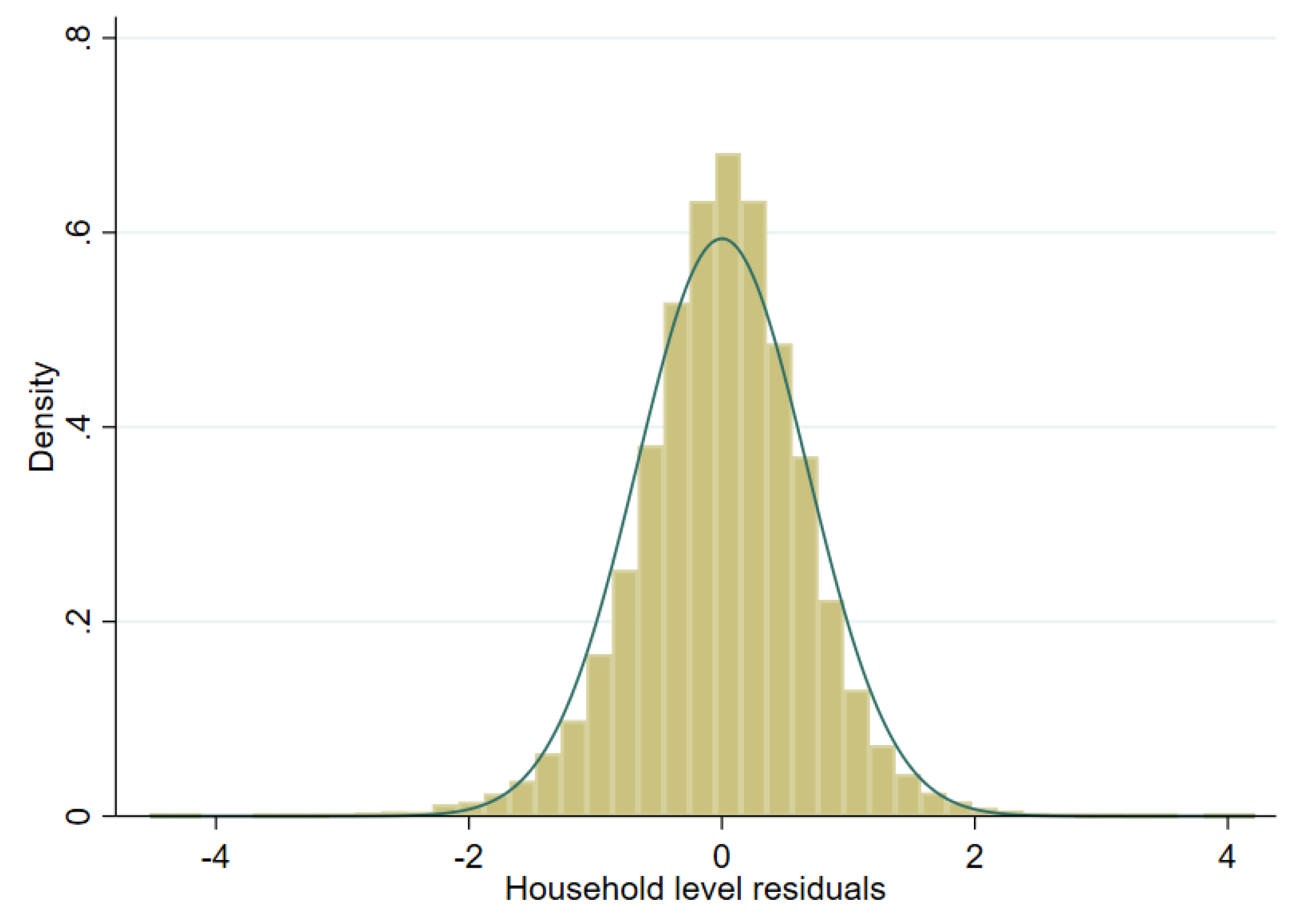
Model selection is conducted using the first sample drawn from the scenario detailed in the previous section. The target variable is household per capita income. However, this variable is highly skewed and to achieve an approximately normal distribution we test three transformations: (i) natural logarithm (in any given sample, roughly 11 observations have an income of 0, these are assigned an income of 1 prior to transformation), (ii) log-shift transformation, and (iii) Box-Cox transformation of the natural logarithm (for further details on transformations, see Tzavidis et al. [7]). As one can see in Figure 6, Figure 7 and Figure 8 for a single sample (from a two-stage clustered design), the Box-Cox transformation, as well as the log shift, fix the skewness in the distribution of model residuals that appears after taking the natural logarithm of per capita income.
The goal of the model selection process is to arrive at a model that only includes stable covariates. Under each transformation, model selection is done using a least absolute shrinkage and selection operator, commonly known as lasso, where the candidates for covariates include household characteristics and characteristics at the PSU, municipal and state level. The model is selected using 20 fold cross validation and shrinkage parameter λ that is within 1 standard error of the one that minimizes the cross validated MSE. Two models are selected: (i) a model that includes household characteristics and characteristics at the PSU, municipal, and state levels and (ii) another model that only includes characteristics at the PSU, municipal and state levels. The second model is used for the unit-context approach. All household level characteristics that are also included as aggregates at the PSU, municipality, and state levels have been previously standardized to ensure that these have mean 0 and standard deviation 1 for each PSU, municipality and state, respectively. Note that aggregated covariates have been obtained from the “census”, thus, the aggregated covariates will be the same within the sample and the census. The lasso model selection process applied here ignores the error structure presented in (1) and (2) and does not ensure that selected covariates will be significant under the assumed models. Consequently, after the initial lasso model selection, model (1) is fit using Henderson’s Method III (with sampling weights) and random effects specified at the municipality level. Because the resulting model may still include covariates that are not significant under the fitted model, all non-significant (at the 1% level) covariates are removed sequentially, starting with the least significant covariate, then the model is fit again without the covariate, and the process is repeated until all covariates in the model are significant at the 1% level. Finally, we check for multicollinearity and remove covariates with a variance inflation factor (VIF) above 3.
Fitted models using the first sample and the described model selection are presented in Table A1 and Table A2 in the Appendix A. Since in small area estimation models are used for prediction, assessing the predictive power of the model is important. This may be measured using the coefficient of determination, R 2 [7]. For the household level model used in this exercise, the R 2 is close to 0.45 while that of the unit-context model centers around 0.25.
Figure 9, Figure 10 and Figure 11 represent checks on the normality assumptions using normal Q-Q-plots of household level residuals and estimated area effects for the onefold unit level model with random municipality location effects. The resulting plots for the unit-context models can be seen in the Appendix A Figure A1, Figure A2 and Figure A3. The natural logarithm transformation (Figure 9) presents evidence of deviation from normality. Marhuenda et al. [8] notes in applications that use real data the exact fit to a distribution is barely met; however, the Box-Cox and log-shift transformations provide considerably better normal approximations, see Figure 10 and Figure 11. Box-Cox and log-shift transformations are available under R’s sae package as well as under Stata’s sae package. In the World Bank’s PovMap software, the only available transformation was natural logarithm. However, PovMap does allow for drawing residuals from the empirical distribution as well as from a Student’s t distribution.

4.3. Results

Once the models to be used have been selected and L = 500 samples under two-stage sampling described in Section 4.1 have been taken from the “census” created using the Mexican Intra Censal Survey of 2015, we obtain estimates using the different considered models. The target parameters for this simulation are mean welfare and the FGT class of decomposable poverty measures defined by Foster et al. [29] for α = 0 , 1 , 2 , for the municipalities present in the census. The true values of the target parameters at the municipal level are based on the census data.
As a first step, we compare results using the three transformations discussed in the previous section. Figure 12 and Figure 13 show box plots of empirical absolute relative bias and MSE of CensusEB estimates of poverty rates based on model (1) under each transformation. The Box-Cox and log-shift transformation yield estimates that are not only less biased, but also result with a lower empirical design MSE. As can be seen in the results from the first 3 columns in Table 2, the log-shift transformation yields aggregate results somewhat preferable to the Box-Cox. Additionally, in Table 2, it is quite clear that the natural logarithm may actually result in aggregate results that present considerably smaller gains over direct ones and thus model and residual checks should always be done to ensure adequate transformations are used to avoid such an outcome. The rest of the discussion will focus on estimates obtained from the log-shift transformation applied to the two-stage samples (Figures under other transformations are available upon request).
We consider estimators based on one-fold and twofold nested error models, including unit-context (UC) models with only aggregated covariates (all models include a constant term), and direct estimators. Concretely, we consider the following (a table summarizing each method can be found in the Appendix A):
Direct Estimates:
  • Direct estimates from the survey samples for each municipality. These are calculated with weights from the considered design. Specifically, the calculation of FGT indicators under the two-stage design detailed in Section 4.1 using the inclusion probabilities is obtained as:
    τ ^ a d i r e c t = c h p a c h p a c h F a c h ;
    where, p a c h is the inclusion probability for household h in cluster c and in municipality a, and F a c h is the FGT or welfare measure of interest for household h in cluster c and in municipality a. Note that, depending on the sampling strategy, some areas might have zero sample size, and hence no direct estimates can be obtained for those areas.
Unit-level models:
  • C E B a : Model fit is done using Henderson’s Method III (with sampling weights) and estimates are obtained using CensusEB as noted in CMN Corral et al. [16]. The fitted model reads:
    y a c h = x a c h β + z a c α + t a ω + g s λ + η a + ε a c h ;
    where x a c h is a vector of household specific characteristics, z a c contains cluster level characteristics, t a includes municipality level characteristics and g s is composed of state level characteristics. The random effects, η a , are specified at the municipal level.
  • C E B c : Model fit is done using Henderson’s Method III (with sampling weights) and estimates are obtained using Census EB as noted in Corral et al. [16]. The difference with model (1) is that random effects are specified at the PSU level. That is, the fitted model is:
    y a c h = x a c h β + z a c α + t a ω + g s λ + η a c + ε a c h ;
    where, η a c , is a random effect for cluster c within municipality a.
  • C E B a c : Model fit is done using REML and estimates are obtained using CensusEB as in Marhuenda et al. [8]. Fitted model follows:
    (a)
    y a c h = x a c h β + z a c α + t a ω + g s λ + η a + η a c + ε a c h ; random effects are specified at the municipality and PSU level.
    Note that CensusEB estimators based on twofold nested error models are obtained without the use of probability sampling weights and are thus not comparable to those estimators that use survey weights.
  • C E B s a : Similar to C E B a c , however random effects are specified at the municipal and state level. The goal here is to borrow strength from the state for municipalities that are not in the sample which takes a cue from Marhuenda et al. [8].
  • E L L c : under the same model as in 2. In cases where we use a transformation different from the natural logarithm, random location effects and household residuals are drawn from their empirical distribution.
Unit-context models:
  • U C C E B a : Unit-context model originally proposed by Nguyen [9] but with EB, similar to Masaki et al. [12]. Model fit is done using Henderson’s Method III (with sampling weights) and estimates are obtained using CensusEB as noted in Corral et al. [16]. The fitted model follows:
    y a c h = z a c α + t a ω + g s λ + η a + ε a c h .
  • U C C E B a c : Unit-context model fit is done using REML and estimates are obtained using CensusEB as in Marhuenda et al. [8]. The fitted model is:
    y a c h = z a c α + t a ω + g s λ + η a + η a c + ε a c h ;
  • U C C E B s a : Similar to model U C C E B a c ; however, random effects are specified at the municipal and state levels. Just like 5, the goal here is to borrow strength from the state for municipalities that are not in the sample.
  • U C E L L c : ELL estimates under model in U C C E B a , but random effects are specified at the PSU level, as was originally proposed by Nguyen [9] and then by Lange et al. [11]. In cases where we use a transformation different from the natural logarithm, random location effects and household residuals are drawn from their empirical distribution.
    y a c h = z a c α + t a ω + g s λ + η a c + ε a c h .
The chosen measures to evaluate performance of the considered predictors are bias, MSE, and root MSE obtained as:
B i a s τ ^ a j = 1 L l = 1 L ( τ ^ a j ( l ) τ a )
M S E τ ^ a j = 1 L l = 1 L ( τ ^ a j ( l ) τ a ) 2
R M S E τ ^ a j = 1 L l = 1 L ( τ ^ a j ( l ) τ a ) 2
where j stands for one of the methods: C E B a , C E B c , d i r e c t , C E B a c , C E B s a , E L L c , U C C E B a , U C C E B a c , U C C E B s a , and U C E L L c ; τ a denotes the true population parameter for municipality a. Note that, in design-based simulations, there is only one true population parameter because our census is fixed. In model-based simulations, the target parameters are random. Formal evaluation of the MSE estimators is not undertaken here since it is beyond the scope of the exercise and computationally intensive as it would require obtaining a bootstrap MSE for each of the 500 samples.
In Section 3.1, like Marhuenda et al. [8], we noticed how the relative size of the random effects affected the precision of the different methods. The first sample from the simulation experiment under two-stage sampling is used to assess the magnitude of the random effects under the unit level model. The values of σ ^ a c 2 and σ ^ a 2 under the twofold nested error model with a log shift transformation for this sample are equal to 0.021 and 0.013, respectively. The value of σ ^ a c 2 when specifying random effects only at the cluster level is equal to 0.072, and σ ^ a c 2 / σ ^ e 2 is equal to 0.054. When specifying random effects only at the municipality level, σ ^ a 2 is equal to 0.022, and the σ ^ a c 2 / σ ^ e 2 ratio is equal to 0.045.
In Figure 14, we can clearly see that, in general, all SAE methods outperform the direct estimates in terms of design MSE (see Figure A6 in the Appendix A for the untrimmed version of the figure). In terms of design bias (Figure 15), direct estimators are very close to being unbiased under the design and would likely converge to the true estimate as the number of simulations increase. On the other hand, model-based estimators are all biased under the design. The result is similar to the one presented by Marhuenda et al. [8], where gains in MSE for model-based estimators are achieved at the expense of design bias. As an additional check, we add simulations where L = 500 samples are taken, each consisting of a 1% SRS without replacement in every PSU within the fixed census population. Aggregate results for this scenario are presented in column 4 of Table 2 and box plots for MSE and bias are presented in Appendix A Figure A4 and Figure A5, respectively. The first thing to note in these figures is there are fewer extreme outliers when compared to results from the two-stage sample scenario in Figure A6 in the Appendix A. Despite fewer outliers, the results under the additional sampling scenario mimic those from two-stage samples. However, under the two-stage sampling used here, direct estimates for most municipalities are not available across all 500 samples (see Section 4.1). Consequently, direct estimates are not included under the remaining figures that discuss results from the two-stage samples.
Under the simulation experiment with two-stage sampling, the empirical MSE of E L L c estimates, where the location effect has been specified at the PSU level, appear to have a tighter spread than direct estimates (Figure 14). Consequently, though ELL appears to perform relatively well, relative to direct estimates, the number of ELL outliers with a high MSE is considerable and E L L c performs worse than all other small area approaches. This result was not expected, as the FGT0 results for U C E L L c appear to perform better than the traditional E L L c , which has a considerably better model fit (note that, under the MI inspired bootstrap of ELL, a very poor model fit will be heavily penalized and will likely yield noise estimates for U C E L L c that are fare worse than direct estimates in most applications). Nevertheless, U C E L L c does very poorly in terms of true MSE for the estimation of mean welfare, with an MSE that is as large as that of direct estimates, and it is also considerably biased, see Appendix A Table A5. These results also hold under the simulation experiment with the 1% SRS by PSU samples.
As expected, C E B a estimates show a considerably tighter MSE spread than direct estimates, but still with outliers. Another interesting finding is that under CensusEB, but with random effects specified at the PSU level ( C E B c ), the empirical MSE is tighter than that of the direct estimates and also displays better properties than E L L c as seen in Table 2. However, given the discussion in the model-based validation and the results shown here, the results with the random effects at the municipality level are preferred over the ones where the effect is specified at the PSU level.
Perhaps the most surprising result is the low MSE of the U C C E B a method with only contextual variables and the other U C C E B variants, as proposed by Masaki et al. [12]. The results display a tight spread and the results from Table 2 corroborate the finding. Nevertheless, beyond UC models being an alternative if contemporaneous census data is not available, the method presents a couple of advantages over traditional Fay–Herriot (FH) area level models under sampling scenarios that follow a two-stage design like the one considered here. First, as noted toward the end of Section 4.1, the majority of municipalities are represented by 1 PSU and thus have quite small sample sizes which makes the likelihood of direct FGT0 estimates being equal to 0 or 1 much higher. Under these cases, the method from Nguyen [9] is a valid alternative to FH because FH is not applicable in these municipalities with a sampling variance of 0. An additional advantage is that the model can be used for multiple indicators, whereas the FH requires a model for each indicator considered.
Table 2. Aggregate results for 1865 municipalities in “Census” (FGT0)—results from 500 samples.
1234
TransformationBox-CoxNat. log.Log. ShiftLog. Shift
Direct
AAB ( × 100 )11.31411.31411.3149.722
ARMSE ( × 100 )14.05114.05114.05111.997
C E B a c
AAB ( × 100 )6.2778.6426.2735.393
ARMSE ( × 100 )6.5809.1696.5745.964
C E B s a
AAB ( × 100 )6.3828.9536.3805.740
ARMSE ( × 100 )6.6959.4146.6875.997
C E B a
AAB ( × 100 )6.0808.8006.0925.395
ARMSE ( × 100 )6.5849.5256.5896.034
C E B c
AAB ( × 100 )6.2538.6906.2776.054
ARMSE ( × 100 )6.3638.8476.3846.181
E L L c
AAB ( × 100 )6.6858.7816.6856.961
ARMSE ( × 100 )6.8208.8546.8207.087
U C C E B a
AAB ( × 100 )6.1717.5316.0165.982
ARMSE ( × 100 )6.6078.2746.4616.672
U C C E B a c
AAB ( × 100 )6.1217.5965.9985.926
ARMSE ( × 100 )6.4468.1866.3326.652
U C E L L c
AAB ( × 100 )6.2508.0196.2507.581
ARMSE ( × 100 )6.4218.1006.4217.758
U C C E B s a
AAB ( × 100 )6.0027.5395.8755.937
ARMSE ( × 100 )6.4148.2846.2946.570
AAB: Average absolute bias; ARMSE: Average root MSE. ELL under Box-Cox and log shift, model is still for Nat. log., but errors are drawn from the empirical distribution. Columns 1, 2, and 3 under two-stage samples (Section 4.1); Column 4 results are under 1% SRS by PSU, all PSUs are included.
A possible explanation for the good performance of unit-context models under the considered experiments could be due to estimated random effects, where σ ^ a c 2 > σ ^ a 2 , which coincides with the better performing scenario in Section 3.1. However, this observation is likely a coincidence, since the performance of unit-context models depends on the particular covariates included in the model and on the shape of the target indicator. Under the Mexican data with the covariates used, the unit-context model performs rather well. However, the method considerably lags behind all others for estimation of the welfare mean by area. A similar result is observed in the results presented in Section 3.1, see also Table A5 in the Appendix A).
Under the simulations of column 3 of Table 2, the gains in MSE for the unit-context methods appear to come in municipalities with larger populations (similar findings are obtained under the simulations for column 1). This is expected because in our sampling scenarios, municipalities with a larger population are more likely to be included in all the samples. For example, in the census there are 16,293 PSUs spread over 1865 municipalities. The median municipality in the created census has 7 PSUs, and the median municipality in a given two-stage sample is only represented by one PSU. Consequently, it is not surprising the unit-context variants under-perform relative to unit models in terms of bias and MSE in municipalities with smaller populations, as can be observed in Figure 16. For municipalities with larger populations, and hence those likely to consist of more PSUs and more of these PSUs in the sample, direct estimates for FGT0 are more precise and unit-context models begin to catch up to unit models (see Figure A7 in the Appendix A).
Under the simulations from a 1% SRS by PSU, shown in Table 2, column 4 and in the Appendix A Figure A4 and Figure A5, we notice the unit models ( C E B a ) present a slight upward bias that seems to become more pronounced in more populous municipalities (Figure 17). Notice that some bias is acceptable since gains in MSE are achieved at the expense of bias, however in this case the presence of outliers seems to lead to increased upward bias that affects more municipalities as we move to more populous deciles (box-plots for C E B a in Figure 17). Unit-context ( U C C E B a ) models on the other hand, appear to have a downward bias. In the box-plots in Figure 17 for U C C E B a , the bias in lower deciles is downward and as we move to upper deciles the downward bias is considerably reduced.
As noted in Section 3.1, the problem faced by unit-context models is an effect that is somehow similar to omitted variable bias, which is manifested as a lack of linearity (see Figure 18). The true model includes household size at the household level. Consequently, this variable is a determinant of the dependent variable. Household size x a c h can be broken down into z a c h x ¯ a c , thus the omitted component, z a c h , is also a determinant of the dependent variable. The unit-context model only includes the PSU average household size x ¯ a c obtained from the census as a covariate. Figure 19 further presents the issue. Under C E B a , residuals appear to follow a random pattern; however, under U C C E B a households in municipalities represented by only one PSU in the sample will all have the same linear fit. This manifests itself in the figures for U C C E B a as a column of vertical dots. The problem can also be observed in Figure 20 where the households within municipalities with just one PSU in the sample will have the same linear fit. More specifically, all the points corresponding to different households from the same PSU become superposed in Figure 20 right, and for those municipalities with just one PSU, there is a single point representing the same predicted value for all the households in that municipality.
To check whether the upward bias of estimators based on unit-level models is due to deviations from model assumptions, specifically deviation from normality, we apply a normalization transformation called ordered quantile normalization [31] (employed also by Masaki et al. [12]). In the absence of tied values the transformation is guaranteed to produce a normally distributed transformed data. The transformation is of use only for FGT0 because it cannot be fully reversed 1 to 1 without the original data and thus one has to extrapolate values not observed in the original data (ibid) (the original functional transformation is only defined when a given value is in the observed original data [31]). The result for this transformation can be seen in Figure 21, and it shows that the deviation from normality may be an issue in our models. The previously observed upward bias in the C E B a models is less evident in these results. However, now that the deviation from normality is less of an issue, the U C C E B a models show a clear downward bias. The figure adds further evidence of a possible bias inherent in the U C C E B a model offsetting the bias due to the deviation from the model’s assumptions—in this case normality. Offsetting of biases is not guaranteed to always occur.
As an additional check, we also performed a hybrid experiment that consists in using the census data created in Section 4.1 and a 5% SRS from each PSU to construct a synthetic census based on a twofold model. The 5% SRS sample is used to select a model with all eligible covariates (household and aggregate) following the same process described in Section 4.2. Using the model’s resulting parameter estimates from a twofold model as in (2), we create a new welfare vector in the census for all households. Then a unit-context model and a new unit model are selected, once again following the process described in Section 4.2 using the first out of 500 samples where 1% SRS by PSU is selected. This is done to remove the issue of outliers from the data and to ensure that the data generating process follows the one assumed in Equation (2). The simulation removes the potential misspecification due to deviations from normality in the data and allows us to isolate the problem present in the unit-context model ( U C C E B a ).
Results for the new hybrid simulations are presented in Figure 22 and Figure 23. Note that in this simulation, where we have removed the normality issue, the upward bias that was present in the unit level model ( C E B a ) is no longer evident. On the other hand, the previously suspected downward bias of the unit context models ( U C C E B a ) is salient, as can be seen in Figure 22 and by municipality deciles sorted by population in Figure 24. Note that under the U C C E B a model more than 75% of the municipalities present a downward bias (Figure 22). This finding is aligned to what we observed in Figure 17. However, because there is no deviation from normality in the hybrid simulation, the downward bias of the unit-context models ( U C C E B a ) is never offset, and is quite considerable and leading to substantially larger empirical MSEs for the unit context models (Figure 25). Simulations were repeated, where, instead of performing model selection, the selected model for CEB estimators contains exactly the same covariates as those used to generate the welfare, and considering only the area aggregates for UC models. This was done just to check whether the observed biases could be due to model misspecification, in the sense that the selected covariates are different from those in the true model. Results were very similar to those observed in the previous hybrid simulation with a model selection step. Hence, the results suggest deviations from the assumed model are an issue and the countering of biases is what is driving the seemingly good results for unit-context models in the two-stage sampling scenario, highlighting the importance of proper data transformations and model selection to ensure that model assumptions hold when using Census EB methods.
Given the direction of the bias of unit-context models is not known a priori (see how under the simulations presented in Figure 1 and Figure 2, the method appears to be upward biased)—and that these might present high bias—unit-context models are unlikely to be preferred over traditional FH models when the census auxiliary data are not aligned to survey microdata, unless the calculation of variances of direct estimators, to be used in the FH model, is not possible for various locations, as noted before. This bias appears also for other measures of welfare, and particularly for ELL variants of the unit-context models. In this case, benchmarking is not a recommended procedure for correcting the bias, since it may not help. EB estimators are approximately model unbiased and optimal in terms of minimizing the MSE for a given area, thus when adjusted afterwards for benchmarking, that is, so that these match usual estimates at higher aggregation levels, the optimal properties are lost and estimators usually become worse in terms of bias and MSE under the model. When benchmarking adjustments are large, as those likely required by UC variants, it is an indication that the model does not really hold for the data. In the case of UC models, we have shown that the model will not hold due to omitted variable bias.
Furthermore, note bias can lead to considerable re-ranking of locations and thus a limit on the acceptable bias should usually be determined according to need. This is of particular importance when determining priorities across areas based on small area estimates. If an area’s true poverty rate is 50% and the method yields an estimator of 10% due to a biased model, there is a real risk that this area may not be given assistance when needed. Molina [10] suggests 5 or 10 percent of absolute relative bias as an acceptable threshold. An additional problem for unit-context models in many applications is it is not possible to match census and survey PSUs; in some cases it is due to confidentiality reasons and in others it is due to different sampling frames used for the survey. The latter is something that is likely to affect applications where census and surveys correspond to different years. Under these scenarios, unit-context models are unlikely to be superior to FH and alternative area models.

5. Conclusions

In this paper, we have illustrated that one of the most important aspects of SAE applications with Census EB methods under unit models is selecting a proper model; especially the issue of data transformation. Such a finding is not new, and has been quite often echoed by others in the area (see Tzavidis et al. [7], Marhuenda et al. [8], Molina and Marhuenda [26]). Here we show how data transformations can lead to improved results. For example, under onefold nested error models, the aggregate gains from moving to a log-shift transformation as opposed to just taking the natural logarithm are close to 30 percent in terms of MSE. Nevertheless, as Marhuenda et al. [8] note, finding an appropriate transformation is not always straightforward and the resulting data could stray from normality which would lead to biased estimates as we also find here. Consequently, model checks and residual analysis are something that every SAE application should include in order to test if the model’s assumptions are not completely invalidated. In case of data deviating from model assumptions, the model should be changed accordingly. For instance, in case of area outliers, fixed effects could be included for those outlying areas in the model to reduce the design bias. If their sample sizes are not too small, the efficiency of the resulting model-based estimates might be acceptable in this case, even if specific model parameters are specific to these areas.
Second, we have validated SAE applications under model-based simulation and design-based simulation methods. Under model-based validation, where the data generating process follows a twofold nested error model, we note the ELL method still performs poorly in terms of MSE even with contextual level variables. The result is most evident in scenarios where area random effects are larger than cluster random effects, since contextual variables do not explain a sufficient amount of the area’s variability. Issues regarding the underestimation of this noise under ELL are not evaluated here, but should be considered by future practitioners, particularly when the noise is estimated under the MI inspired bootstrap method (see Marhuenda et al. [8], Das and Chambers [14], Corral et al. [16] ). On the other hand, model-based simulations conducted here provide further evidence to the finding from Marhuenda et al. [8] that misspecification of the model under the onefold CensusEB, i.e., modeling random effects at the area level only, when the true model has cluster and area level random effects, with clusters nested within areas, entails virtually no loss of efficiency when estimating area level welfare-based indicators.
Under design-based validation, where the sampling strategy mimics real world scenarios such as those implemented under LSMS surveys, SAE methods present improvements over direct estimators. We have also investigated estimators based on unit-context models, originally proposed by Nguyen [9], which can be applied when census auxiliary data at the household level is not valid. Given that under the two-stage samples used, many municipalities, which are the target areas, are represented by a small number of observations (or even zero), these data are not always suitable for FH area level models. Despite model-based simulations yielding poor results in terms of bias for unit-context models, the CensusEB variant does considerably better than the ELL variant under the design-based simulations. The reason for the positive results is shown to be due to the bias that is inherent in the unit-context model, which was being offset by bias due to deviations from normality. This offset is something that is not guaranteed to occur in all scenarios because the direction of the bias of unit-context models is not known a priori. In simulations where deviations from normality are not an issue, the bias of the unit-context method becomes quite clear. Additionally, the method’s performance is contingent upon the number of subdomains present in the domain. Moreover, PSUs or subdomains must be matched across census and survey for unit-context models, something that is not always feasible. Finally, since the direction and size of the bias of the unit-context model are not known beforehand, the models may be considered an alternative to FH and other area level models only when area level models are not applicable, like in our design-based experiment with the more realistic two-stage sampling.

Author Contributions

Writing (original draft), P.C., K.H. and K.M.; Writing (review and editing), I.M. All authors have read and agreed to the published version of the manuscript.

Funding

This research was funded by Ministry of Economy, Industry and Competitiveness grant numbers MTM2015-69638-R (MINECO/FEDER, UE) and MTM2015-72907-EXP.

Institutional Review Board Statement

Not applicable.

Informed Consent Statement

Not applicable.

Data Availability Statement

Not applicable.

Acknowledgments

The authors acknowledge financial support from the World Bank. We thank Sandra Carolina Segovia for research assistance. We thank J.N.K. Rao for comments and suggestions. We also thank Roy van der Weide, Alexandru Cojocaru, David Newhouse, and Samuel Freije-Rodriguez for comments. Additionally, we thank Carolina Sanchez and Roberta Gatti for providing support and space to pursue this work. Finally, we thank the Global Solutions Group on Data for Policy, as well as all attendants of the Summer University courses on Small Area Estimation. Any error or omission is the authors’ responsibility alone.

Conflicts of Interest

The authors declare no conflict of interest.

Abbreviations

The following abbreviations are used in this manuscript:
ModelDescription
LSMSLiving Standards Measurement Study
MSEMean Squared Error
MDGsMillennium Development Goals
SDGsSustainable Development Goals
SAESmall Area Estimation
ELLElbers, Lanjouw and Lanjouw (2003)
MRMolina and Rao (2010)
PSUsPrimary Sampling Units
EBEmpirical Best
CMNCorral, Molina and Nguyen (2020)
MIMultiple Imputation
EBLUPEmpirical Best Linear Unbiased Predictor
REMLRestricted Maximum Likelihood
H3Henderson Method III
CBEBClustered Bootstrap EB
FHFay-Herriot
GISGeographic Information System
FGTFoster, Greer and Thorbecke (1984)
AABAverage Absolute Bias
ARMSEAverage root MSE
INEGIInstituto Nacional de Estadistica y Geografia
ICTInformation and Communication Technologies
RSERelative Standard Error
SRSSimple random sampling
ICCIntra-cluster Correlation
DEFFDesign Effect
PPSProbability Proportional to Size
VIFVariance Inflation Factor
UCUnit-Context

Appendix A

Figure A1. Normal Q-Q-plot of one-fold unit-context model and predicted subdomain effects (Nat. log. transformation).
Mathematics 09 02780 g0a1
Figure A2. Normal Q-Q-plot of one-fold unit-context model and predicted subdomain effects (log-shift transformation).
Mathematics 09 02780 g0a2
Figure A3. Normal Q-Q-plot of one-fold unit-context model and predicted subdomain effects (Box-Cox of Nat. log transformation).
Mathematics 09 02780 g0a3
Figure A4. Box plots of empirical design MSE for FGT0 under 1% SRS by PSU sampling (Nat. log. shift transformation).
Mathematics 09 02780 g0a4
Figure A5. Box plots of empirical design bias for FGT0 under 1% SRS by PSU sampling (Nat. log. shift transformation).
Mathematics 09 02780 g0a5
Figure A6. Box plots of empirical design MSE for FGT0 under two-stage sampling (Nat. log. shift transformation).
Mathematics 09 02780 g0a6
Figure A7. Average empirical MSE for FGT0 under two-stage sampling by municipality population deciles (Nat. log. shift transformation).
Mathematics 09 02780 g0a7
Table A1. Unit level model—under log shift transformation.
VariableCoefficientStd. Error
PSU HH head age−0.0726 ***(0.00700)
PSU % hh with internet0.133 ***(0.00937)
PSU % of hh with television0.141 ***(0.00864)
Head’s age−0.00127 ***(0.000406)
HH owns a cellphone0.214 ***(0.0155)
HH owns a computer0.190 ***(0.0178)
Number of hh members−0.118 ***(0.00315)
HH has access to internet0.105 ***(0.0181)
Male HH head0.0640 ***(0.0136)
Max. education is tertiary0.393 ***(0.0156)
Share of adult hh members0.688 ***(0.0247)
State % of male head hh−0.0683 ***(0.00870)
State share of elderly population−0.0514 ***(0.0120)
HH owns a washing machine0.119 ***(0.0136)
Constant6.984 ***(0.0351)
Observations23,516
Adj. R 2 0.445
σ a 2 0.0220
σ a 2 / σ e 2 0.0452
Standard errors in parentheses *** p < 0.01, ** p < 0.05, * p < 0.1.
Table A2. Unit-context model—under log shift transformation.
VariableCoefficientStd. Error
PSU avg. hh number of members−0.127 ***(0.0105)
PSU share of male headed households−0.0595 ***(0.00976)
PSU share of households with max. tertiary education0.219 ***(0.0105)
PSU avg. share of elderly−0.0760 ***(0.00783)
PSU avg. share of female members−0.0283 ***(0.00913)
Municipal share of hh owning a television0.168 ***(0.0116)
State share of hh owning a computer0.123 ***(0.0110)
Constant7.353 ***(0.0104)
Observations23,516
Adj. R 2 0.253
σ a 2 0.0234
σ a 2 / σ e 2 0.0357
Standard errors in parentheses *** p < 0.01, ** p < 0.05, * p < 0.1.
Table A3. Aggregate results for 1865 municipalities of Mexico (FGT1)—results from 500 samples.
1234
TransformationBox-CoxNat. log.Log. ShiftLog. Shift
Direct
AAB ( × 100 )5.5495.5495.5494.773
ARMSE ( × 100 )6.9756.9756.9755.943
C E B a c
AAB ( × 100 )3.5835.8433.6993.210
ARMSE ( × 100 )3.7476.2173.8673.523
C E B s a
AAB ( × 100 )3.6656.0683.7733.417
ARMSE ( × 100 )3.8306.3863.9413.553
C E B a
AAB ( × 100 )3.4275.8893.5333.205
ARMSE ( × 100 )3.6936.4063.8073.553
C E B c
AAB ( × 100 )3.5485.7793.6803.556
ARMSE ( × 100 )3.6145.9043.7463.631
E L L c
AAB ( × 100 )4.2095.7834.2094.516
ARMSE ( × 100 )4.3005.8444.3004.600
U C C E B a
AAB ( × 100 )3.3294.5893.1663.319
ARMSE ( × 100 )3.5435.0803.4003.668
U C C E B a c
AAB ( × 100 )3.2874.6063.1653.284
ARMSE ( × 100 )3.4514.9983.3443.653
U C E L L c
AAB ( × 100 )3.4634.7303.4634.522
ARMSE ( × 100 )3.5744.7973.5744.637
U C C E B s a
AAB ( × 100 )3.2654.6283.1363.319
ARMSE ( × 100 )3.4705.1223.3573.638
AAB: Average absolute bias; ARMSE: Average root MSE. ELL under Box-Cox and log shift, model is still for Nat. log., but errors are drawn from the empirical distribution. Columns 1, 2, and 3 under two-stage samples (Section 4.1); Column 4 results are under 1% SRS by PSU, all PSUs are included.
Table A4. Aggregate results for 1865 municipalities of Mexico (FGT2)—results from 500 samples.
1234
TransformationBox-CoxNat. log.Log. ShiftLog. Shift
Direct
AAB ( × 100 )3.9013.9013.9013.441
ARMSE ( × 100 )5.0175.0175.0174.361
C E B a c
AAB ( × 100 )2.4324.1352.5662.267
ARMSE ( × 100 )2.5394.4212.6822.476
C E B s a
AAB ( × 100 )2.4984.2892.6172.411
ARMSE ( × 100 )2.6054.5352.7312.501
C E B a
AAB ( × 100 )2.3274.1442.4342.259
ARMSE ( × 100 )2.4984.5402.6192.492
C E B c
AAB ( × 100 )2.4154.0732.5552.514
ARMSE ( × 100 )2.4624.1732.6022.564
E L L c
AAB ( × 100 )3.0534.0853.0533.364
ARMSE ( × 100 )3.1244.1373.1243.435
U C C E B a
AAB ( × 100 )2.3543.2002.1852.329
ARMSE ( × 100 )2.4823.5582.3352.547
U C C E B a c
AAB ( × 100 )2.3063.2042.1822.303
ARMSE ( × 100 )2.4063.4922.2992.535
U C E L L c
AAB ( × 100 )2.4783.2972.4783.312
ARMSE ( × 100 )2.5603.3522.5603.405
U C C E B s a
AAB ( × 100 )2.3073.2282.1772.334
ARMSE ( × 100 )2.4313.5912.3192.532
AAB: Average absolute bias; ARMSE: Average root MSE. ELL under Box-Cox and log shift, model is still for Nat. log. but errors are drawn from the empirical distribution. Columns 1, 2, and 3 under two-stage samples (Section 4.1); Column 4 results are under 1% SRS by PSU, all PSUs are included.
Table A5. Aggregate results for 1865 municipalities of Mexico (Mean income)—results from 500 samples.
1234
TransformationBox-CoxNat. log.Log. ShiftLog. Shift
Direct
AAB ( × 100 )38,838.4438,838.4438,838.4430,028.16
ARMSE ( × 100 )54,351.7154,351.7154,351.7141,841.21
C E B a c
AAB ( × 100 )18,374.6145,904.5318,276.2616,908.87
ARMSE ( × 100 )19,998.5648,531.7619,899.9619,569.77
C E B s a
AAB ( × 100 )19,574.3845,440.0719,452.7518,426.15
ARMSE ( × 100 )21,207.4147,861.5921,069.7419,745.09
C E B a
AAB ( × 100 )18,146.6643,445.3818,158.0917,016.17
ARMSE ( × 100 )20,596.5447,108.7020,591.8519,967.33
C E B c
AAB ( × 100 )19,048.9046,845.9119,093.2421,112.72
ARMSE ( × 100 )19,534.0647,576.3219,570.1621,653.29
E L L c
AAB ( × 100 )32,576.3048,594.3632,576.3044,808.60
ARMSE ( × 100 )33,650.5949,018.6233,650.5945,504.33
U C C E B a
AAB ( × 100 )31,330.7067,999.5930,715.1329,647.72
ARMSE ( × 100 )33,900.1472,555.9733,309.2733,513.86
U C C E B a c
AAB ( × 100 )32,718.3169,364.8331,893.1529,700.46
ARMSE ( × 100 )34,599.5472,841.4033,823.6833,765.53
U C E L L c
AAB ( × 100 )53,184.1473,673.7053,184.1471,189.32
ARMSE ( × 100 )54,672.1674,068.4254,672.1672,282.49
U C C E B s a
AAB ( × 100 )33,148.5469,355.8232,296.1529,642.77
ARMSE ( × 100 )35,502.1873,879.7334,677.9633,217.28
AAB: Average absolute bias; ARMSE: Average root MSE. ELL under Box-Cox and log shift, model is still for Nat. log. but errors are drawn from the empirical distribution. Columns 1, 2, and 3 under two-stage samples (Section 4.1); Column 4 results are under 1% SRS by PSU, all PSUs are included.
Table A6. Different models tested.
ModelDescription
C E B a One-fold CensusEB unit model with location effects specified at the municipality level
C E B c One-fold CensusEB unit model with location effects specified at the PSU level
C E B a c Two-fold CensusEB unit model with location effects specified at the municipality and PSU level
C E B s a Two-fold CensusEB unit model with location effects specified at the state and municipality level
E L L c One-fold ELL unit model with location effects specified at the PSU level
U C C E B a One-fold CensusEB unit-context model with location effects specified at the municipality level
U C C E B a c Two-fold CensusEB unit-context model with location effects specified at the municipality and PSU level
U C C E B s a Two-fold CensusEB unit-context model with location effects specified at the state and municipality level
U C E L L c One-fold ELL unit-context model with location effects specified at the PSU level

Appendix B

Appendix B.1. Omitted Variable Bias under Unit-Context Models

Consider that data are generated as:
y a h = β 0 + β 1 x a h 1 + + β p x a h p + η a + e a h ; h = 1 , , N a ; a = 1 , , A
Let us decompose x a h k as follows:
x a h k = x a h k X ¯ a k + X ¯ a k , where X ¯ a k = N a 1 h = 1 N a x a h k is the population mean of x a h k in area a. However, under unit-context model we fit:
y a h = α 0 + α 1 X ¯ a 1 + + α p X ¯ a p + η a + e a h ; h = 1 , , N a ; a = 1 , , A
Note that here we are omitting variables:
x ˜ a h k = x a h k X ¯ a k ; k = 1 , , p
Let us write model (A1) in matrix notation, for the sample data. For this we define the vectors:
y a = y a 1 y a n a , X a = 1 x a 1 1 x a 1 p 1 x a n a 1 x a n a p , β = β 0 β 1 β p , e a = e a 1 e a n a
Then, the model is given by:
y a = X a β + 1 n a η a + e a , a = 1 , , A
Finally, define:
y = y 1 y A , X = X 1 X A , Z = 1 n 1 1 n A , η = η 1 η A e a = e a 1 e a n a
where 1 n A is an n A × 1 column of ones.
Then the model in (A1) may be written as:
y = X β + Z η + e
On the other hand, for model (A2) we define:
X ¯ = 1 n 1 X ¯ 1 1 1 n 1 X ¯ 1 p 1 n 1 1 n A X ¯ A 1 1 n A X ¯ 1 p 1 n A
Then model (A2) can be written as, for α = α 0 , α 1 , , α p :
y = X ¯ α + Z η + e
the WLS estimator of α in model (A2):
α ^ U C = X ¯ V 1 X ¯ 1 X ¯ V 1 y
However, y actually follows model (A1), that is:
y = X ˜ β ( 0 ) + X ¯ β + Z η + e
where
β ( 0 ) = β 0 β p , X ˜ = X ˜ 1 X ˜ A , X ˜ a = x a 1 1 X ¯ a 1 x a 1 p X ¯ a p x a n a 1 X ¯ a 1 x a n a p X ¯ a p
replacing (A4) in to (A3), we get:
α ^ U C = X ¯ V 1 X ¯ 1 X ¯ V 1 X ¯ β + X ¯ V 1 X ¯ 1 X ¯ V 1 X ˜ β ( 0 ) + X ¯ V 1 X ¯ 1 X ¯ V 1 ( Z η + e )
Taking expectations, and since E η = 0 and E e = 0 , we get:
E α ^ U C = β + B α ^ U C
where the bias is equal to:
B α ^ U C = X ¯ V 1 X ¯ 1 X ¯ V 1 X ˜ β ( 0 )
where
X ¯ V 1 X ¯ = 1 σ η 2 a γ a a γ a X ¯ a 1 a γ a X ¯ a p a γ a X ¯ a 1 a γ a X ¯ a 1 2 a γ a X ¯ a 1 X ¯ a p a γ a X ¯ a p a γ a X ¯ a 1 X ¯ a p a γ a X ¯ a p 2
and where
γ a = σ η 2 σ η 2 + σ e 2 n a
Additionally, we obtain
X ¯ V 1 X ˜ β ( 0 ) = a 1 n a V a 1 X ˜ a β ( 0 ) a X ¯ a 1 1 n a V a 1 X ˜ a β ( 0 ) a X ¯ a p 1 n a V a 1 X ˜ a β ( 0 )
noting that:
1 n a V a 1 X ˜ a = 1 σ η 2 γ a n a 1 n a x ˜ a
where x ˜ a = x ˜ a 1 , , x ˜ a p , with
x ˜ a k = 1 n a h S a x a h k X ¯ a k = x ¯ a k X ¯ a k
and where S a is the survey sample households in area a. Therefore,
X ¯ V 1 X ˜ β ( 0 ) = 1 σ η 2 a γ a k x ˜ a k β k a γ a X ¯ a 1 k x ˜ a k β k a γ a X ¯ a p k x ˜ a k β k
Finally, the bias is given by:
B α ^ U C = a γ a a γ a X ¯ a 1 a γ a X ¯ a p a γ a X ¯ a 1 a γ a X ¯ a 1 2 a γ a X ¯ a 1 X ¯ a p a γ a X ¯ a p a γ a X ¯ a 1 X ¯ a p a γ a X ¯ a p 2 1 a γ a k x ˜ a k β k a γ a X ¯ a 1 k x ˜ a k β k a γ a X ¯ a p k x ˜ a k β k
Consequently, the bias of α ^ U C is due to the discrepancy between the sample mean of a given covariate and the population mean of that covariate, x ˜ a k = x ¯ a k X ¯ a k .

Appendix B.2. Bias of Individual Predictors under Unit-Context Models

Under model (A2),
y a h = X ¯ a α + η a + e a h
the conditional expectation under model (A2) for h S a is:
μ a h | s U C = E y a h | y s = X ¯ a α + η ˜ a , for η ˜ a = γ a y ¯ a X ¯ a α
Then, and replacing α with its estimate, α ^ U C
μ a h | s U C = X ¯ a α ^ U C + γ a y ¯ a X ¯ a α ^ U C = γ a y ¯ a + 1 γ a X ¯ a α ^ U C
and taking its expectation, we get:
E μ a h | s U C = γ a E y ¯ a + 1 γ a X ¯ a E α ^ U C ,
where E y ¯ a = x ¯ a β and E α ^ U C = β + B α ^ U C . Consequently,
E μ a h | s U C = X ¯ a β + γ a x ¯ a X ¯ a β + ( 1 γ a ) X ¯ a B α ^ U C
Note that once again, the discrepancy between the sample and population means play a role in the bias.

References

  1. Rao, J.; Molina, I. Small Area Estimation, 2nd ed.; John Wiley & Sons: Hoboken, NJ, USA, 2015. [Google Scholar]
  2. Ghosh, M.; Rao, J. Small area estimation: An appraisal. Stat. Sci. 1994, 9, 55–76. [Google Scholar] [CrossRef]
  3. Fay, R.E., III; Herriot, R.A. Estimates of income for small places: An application of James-Stein procedures to census data. J. Am. Stat. Assoc. 1979, 74, 269–277. [Google Scholar] [CrossRef]
  4. Torabi, M.; Rao, J. On small area estimation under a sub-area level model. J. Multivar. Anal. 2014, 127, 36–55. [Google Scholar] [CrossRef]
  5. Molina, I.; Rao, J. Small area estimation of poverty indicators. Can. J. Stat. 2010, 38, 369–385. [Google Scholar] [CrossRef] [Green Version]
  6. Elbers, C.; Lanjouw, J.O.; Lanjouw, P. Micro—Level estimation of poverty and inequality. Econometrica 2003, 71, 355–364. [Google Scholar] [CrossRef]
  7. Tzavidis, N.; Zhang, L.C.; Luna, A.; Schmid, T.; Rojas-Perilla, N. From start to finish: A framework for the production of small area official statistics. J. R. Stat. Soc. Ser. A Stat. Soc. 2018, 181, 927–979. [Google Scholar] [CrossRef] [Green Version]
  8. Marhuenda, Y.; Molina, I.; Morales, D.; Rao, J. Poverty mapping in small areas under a twofold nested error regression model. J. R. Stat. Soc. Ser. A Stat. Soc. 2017, 180, 1111–1136. [Google Scholar] [CrossRef]
  9. Nguyen, V.C. A Method to Update Poverty Maps. J. Dev. Stud. 2012, 48, 1844–1863. [Google Scholar] [CrossRef]
  10. Molina, I. Desagregación de datos en Encuestas de Hogares: Metodologías de Estimación En áreas Pequeñas. 2019, Series Estudios Estadísticos, No 97, (LC/TS.2018/82/Rev.1), Santiago, Comisión Económica para América Latina y el Caribe, (CEPAL). Available online: https://www.cepal.org/es/publicaciones/44214-desagregacion-datos-encuestas-hogares-metodologias-estimacion-areas-pequenas (accessed on 24 October 2021).
  11. Lange, S.; Pape, U.J.; Pütz, P. Small Area Estimation of Poverty under Structural Change. World Bank Policy Res. Work. Pap. 2018. Number 8472. Available online: https://papers.ssrn.com/sol3/papers.cfm?abstract_id=3238306 (accessed on 24 October 2021).
  12. Masaki, T.; Newhouse, D.; Silwal, A.R.; Bedada, A.; Engstrom, R. Small Area Estimation of Non-Monetary Poverty with Geospatial Data. World Bank Policy Res. Work. Pap. 2020. Number 9383. Available online: https://openknowledge.worldbank.org/handle/10986/34469 (accessed on 24 October 2021).
  13. Battese, G.E.; Harter, R.M.; Fuller, W.A. An Error-Components Model for Prediction of County Crop Areas Using Survey and Satellite Data. J. Am. Stat. Assoc. 1988, 83, 28–36. [Google Scholar] [CrossRef]
  14. Das, S.; Chambers, R. Robust mean-squared error estimation for poverty estimates based on the method of Elbers, Lanjouw and Lanjouw. J. R. Stat. Soc. Ser. A Stat. Soc. 2017, 180, 1137–1161. [Google Scholar] [CrossRef]
  15. Elbers, C.; Lanjouw, J.O.; Lanjouw, P. Micro-Level Estimation of Welfare. World Bank Policy Res. Work. Pap. 2002. Number 2911. Available online: https://elibrary.worldbank.org/doi/abs/10.1596/1813-9450-2911 (accessed on 24 October 2021).
  16. Corral, P.; Molina, I.; Nguyen, M.C. Pull Your Small Area Estimates up by the Bootstraps. J. Stat. Comput. Simul. 2021, 91, 3304–3357. [Google Scholar]
  17. Tarozzi, A.; Deaton, A. Using census and survey data to estimate poverty and inequality for small areas. Rev. Econ. Stat. 2009, 91, 773–792. [Google Scholar] [CrossRef] [Green Version]
  18. Van Buuren, S. Flexible Imputation of Missing Data; Chapman and Hall/CRC: Boca Raton, FL, USA, 2018. [Google Scholar]
  19. González-Manteiga, W.; Lombardía, M.J.; Molina, I.; Morales, D.; Santamaría, L. Bootstrap mean squared error of a small-area EBLUP. J. Stat. Comput. Simul. 2008, 78, 443–462. [Google Scholar] [CrossRef]
  20. Van der Weide, R. GLS Estimation and Empirical Bayes Prediction for Linear Mixed Models with Heteroskedasticity and Sampling Weights: A Background Study for the POVMAP Project. World Bank Policy Res. Work. Pap. 2014. Number 7028. Available online: https://papers.ssrn.com/sol3/papers.cfm?abstract_id=2495175 (accessed on 24 October 2021).
  21. Huang, R.; Hidiroglou, M. Design consistent estimators for a mixed linear model on survey data. Proc. Surv. Res. Methods Sect. Am. Stat. Assoc. 2003, 6, 1897–1904. [Google Scholar]
  22. Henderson, C.R. Estimation of variance and covariance components. Biometrics 1953, 9, 226–252. [Google Scholar] [CrossRef]
  23. You, Y.; Rao, J. A pseudo-empirical best linear unbiased prediction approach to small area estimation using survey weights. Can. J. Stat. 2002, 30, 431–439. [Google Scholar] [CrossRef]
  24. Zhao, Q. User Manual for PovMap. World Bank. 2006. Available online: http://siteresources.worldbank.org/INTPGI/Resources/342674-1092157888460/Zhao_ManualPovMap.pdf (accessed on 24 October 2021).
  25. Nguyen, M.C.; Corral, P.; Azevedo, J.P.; Zhao, Q. Sae: A Stata Package for Unit Level Small Area Estimation. World Bank Policy Res. Work. Pap. 2018. Number 8630. Available online: https://papers.ssrn.com/sol3/papers.cfm?abstract_id=3275801 (accessed on 24 October 2021).
  26. Molina, I.; Marhuenda, Y. Sae: An R package for small area estimation. R J. 2015, 7, 81–98. [Google Scholar] [CrossRef] [Green Version]
  27. Guadarrama, M.; Molina, I.; Rao, J. A comparison of small area estimation methods for poverty mapping. Stat. Transit. New Ser. 2016, 1, 41–66. [Google Scholar] [CrossRef] [Green Version]
  28. Molina, I.; Morales, D. Small area estimation of poverty indicators. Estad. E Investig. Oper. 2009, 25, 369–385. [Google Scholar] [CrossRef] [Green Version]
  29. Foster, J.; Greer, J.; Thorbecke, E. A class of decomposable poverty measures. Econom. J. Econom. Soc. 1984, 52, 761–766. [Google Scholar] [CrossRef]
  30. Grosh, M.E.; Muñoz, J. A Manual for Planning and Implementing the Living Standards Measurement Study Survey; The World Bank: Washington, DC, USA, 1996. [Google Scholar]
  31. Peterson, R.A.; Cavanaugh, J.E. Ordered quantile normalization: A semiparametric transformation built for the cross-validation era. J. Appl. Stat. 2019, 47, 2312–2327. [Google Scholar] [CrossRef]
Figure 1. Empirical model bias of FGT0 estimators for σ a c = 0.1 and σ a = 0.05 .
Mathematics 09 02780 g001
Figure 2. Empirical model bias of FGT0 estimators for σ a c = 0.05 and σ a = 0.1 .
Mathematics 09 02780 g002
Figure 3. Empirical model MSE of FGT0 estimators; σ a c = 0.1 and σ a = 0.05 .
Mathematics 09 02780 g003
Figure 4. Empirical model MSE of FGT0 estimators; σ a c = 0.05 and σ a = 0.1 .
Mathematics 09 02780 g004
Figure 5. Omitted variable bias under unit-context models.
Mathematics 09 02780 g005
Figure 6. Histogram of residuals from unit level one-fold nested error model fitted to Nat. log. of per capita income (municipal random effects).
Mathematics 09 02780 g006
Figure 7. Histogram of residuals from unit level onefold nested error model fitted to log-shift transformation of per capita income (municipal random effects).
Mathematics 09 02780 g007
Figure 8. Histogram of residuals from unit level onefold nested error model fitted to Box-Cox of Nat. log. of per capita income (municipal random effects).
Mathematics 09 02780 g008
Figure 9. Normal Q-Q-plot of unit level onefold nested error model—household level and predicted subdomain effects (Nat. log transformation).
Mathematics 09 02780 g009
Figure 10. Normal Q-Q-plot of unit level one-fold nested error model—household level and predicted subdomain effects (log-shift transformation).
Mathematics 09 02780 g010
Figure 11. Normal Q-Q-plot of unit level one-fold nested error model—household level and predicted subdomain effects (Box-Cox of nat. log transformation).
Mathematics 09 02780 g011
Figure 12. Box plots of Census EB FGT0 design bias for unit level one-fold nested error model estimates for fitted model 1 and two-stage samples (Municipal level).
Mathematics 09 02780 g012
Figure 13. Box plots of empirical MSE of unit level onefold nested error model CensusEB FGT0 estimates for fitted model 1 and two-stage samples (Municipal level).
Mathematics 09 02780 g013
Figure 14. Box plots of empirical design MSE for FGT0 under two-stage sampling (Nat. log. shift transformation).
Mathematics 09 02780 g014
Figure 15. Boxplot of empirical design bias for FGT0 under two-stage sampling (Nat. log. shift transformation).
Mathematics 09 02780 g015
Figure 16. Average empirical MSE for FGT0 under two-stage sampling by municipality population deciles (Nat. log. shift transformation).
Mathematics 09 02780 g016
Figure 17. Box plots of design bias under 1% SRS by PSU sampling, by municipality population deciles (Nat. log. shift transformation).
Mathematics 09 02780 g017
Figure 18. Omitted variable bias under unit-context models.
Mathematics 09 02780 g018
Figure 19. Household residuals plotted against linear fit under two-stage sampling (Nat. log. shift transformation).
Mathematics 09 02780 g019
Figure 20. Linear fit plotted against municipalities under two-stage sampling (Nat. log. shift transformation).
Mathematics 09 02780 g020
Figure 21. Box plots of design bias under ordered quantile normalization by municipality population deciles (Two-stage sampling).
Mathematics 09 02780 g021
Figure 22. Box plots of design bias under 1% SRS by PSU sampling (Hybrid simulation).
Mathematics 09 02780 g022
Figure 23. Box plots of empirical MSE under 1% SRS by PSU sampling by municipality population deciles (Hybrid simulation).
Mathematics 09 02780 g023
Figure 24. Box plots of design bias under 1% SRS by PSU sampling, by municipality population deciles (Hybrid simulation).
Mathematics 09 02780 g024
Figure 25. Box-plot of empirical MSE for FGT0 under 1% SRS by PSU sampling by municipality population deciles (Hybrid simulation).
Mathematics 09 02780 g025
Table 1. Aggregate results across areas (FGT0).
1234
Model R 2 ~0.42~0.42~0.42~0.42
σ a 0.050.10.050.1
σ a c 0.10.050.10.05
σ e 0.50.50.50.5
Sample per cluster10 per all clusters10 per all clusters10 per 20% clusters10 per 20% clusters
Population20,00020,000100,000100,000
Direct
AAB ( × 100 )1.7801.7831.8021.795
ARMSE ( × 100 )4.0394.0414.3964.563
C E B a c
AAB ( × 100 )0.0200.0230.0180.023
ARMSE ( × 100 )2.6302.8592.4932.191
C E B a
AAB ( × 100 )0.0200.0240.0210.017
ARMSE ( × 100 )2.6422.8762.5152.237
C E B c
AAB ( × 100 )0.0240.0290.0450.020
ARMSE ( × 100 )2.7933.8854.7312.614
E L L c
AAB ( × 100 )0.2380.2360.1440.139
ARMSE ( × 100 )3.4335.2695.0482.768
U C C E B a
AAB ( × 100 )1.1151.3621.2960.986
ARMSE ( × 100 )3.0743.4043.0682.584
U C C E B a c
AAB ( × 100 )1.1061.3701.2720.929
ARMSE ( × 100 )3.0593.3833.0462.591
AAB: Average absolute bias; ARMSE: Average root MSE.
Publisher’s Note: MDPI stays neutral with regard to jurisdictional claims in published maps and institutional affiliations.

