Combination Synchronization of Fractional Systems Involving the Caputo–Hadamard Derivative

Abstract

The main aim of this paper is to investigate the combination synchronization phenomena of various fractional-order systems using the scaling matrix. For this purpose, the combination synchronization is performed by considering two drive systems and one response system. We show that the combination synchronization phenomenon is achieved theoretically. Moreover, numerical simulations are carried out to confirm and validate the obtained theoretical results.

1. Introduction

Fractional calculus is an old topic, going back to Riemann–Liouville, Leibniz, and Grünwald–Letnikov, where derivatives and integrals are considered of a real or complex order [1,2]. In the last three decades, fractional calculus has gained a lot of interest due to its application in various scientific fields [3,4,5,6]. The fractional derivative is considered an excellent tool for explaining different processes with memory and anomalous diffusion problems compared to the classical derivative [7]. In the literature, there are many famous definitions of fractional derivatives, such as Caputo, Riemann–Liouville, Katugampola, and Hadamard, that have been described and used in many scientific applications [2,8,9]. Nowadays, other fractional definitions have become valuable because of their applications and background. For instance, the Caputo–Hadamard fractional-order derivative is a modified version of the Hadamard fractional-order derivative. More details, including the analysis and application of the Caputo–Hadamard fractional derivative, can be found in [10,11,12]. Furthermore, new results for complicated fractional Caputo–Hadamard systems using various theoretical techniques are presented in [13,14].

Synchronization is a procedure in which two or more systems react with each other, leading to a joint development in some of their dynamic characteristics. These systems are able to adjust their pace and exhibit the same behavior over time. The concept of synchronization in chaotic systems was proposed by Pekora and Carol [15]. Thereafter, the phenomena of synchronization gained a lot of attention from numerous researchers. Due to the growing interest in studying the synchronization phenomena for chaotic dynamical systems, many types of synchronization have been discovered in the literature [16,17,18,19,20].

Recently, Runzi et al. [21] presented a new type of synchronization called combination synchronization. This type of synchronization consists of one response system and two drive systems. Combination synchronization has been applied to widespread applications, especially for various chaotic systems [7,22,23]. Moreover, the combination synchronization phenomenon has also been studied for fractional dynamical systems [24,25,26].

This paper is structured in the following manner: In Section 2, we provide some preliminaries for fractional calculus. Section 3 introduces the main idea of the combination synchronization of fractional-order systems given in this paper and shows that the combination synchronization phenomena are theoretically achieved. To validate the theoretical analysis, numerical simulations are provided in Section 4. Finally, some conclusions are presented in Section 5.

2. Preliminaries

In this section, we reviewed some useful definitions that served as the basis for our present work.

The Caputo fractional derivative of h of order $\varsigma$ was provided by:

$${}^C{\mathcal{D}}_{t_0,t}^{\varsigma }h\left(t\right)={\mathcal{D}}_{t_0,t}^{\varsigma }[h\left(t\right)-h\left(t_0\right)],$$

where ${\mathcal{D}}_{t_0,t}^{\varsigma }$ denotes the Riemann–Liouville fractional derivative:

$${\mathcal{D}}_{t_0,t}^{\varsigma }h\left(t\right)=\frac{1}{\Gamma (1-\varsigma )}\frac{d}{dt}{\int }_{t_0}^t{(t-\nu )}^{-\varsigma }h\left(\nu \right)d\nu .$$

If h was absolutely continuous, then the Caputo fractional derivative could be written in an equivalent form as follows:

$${}^C{\mathcal{D}}_{t_0,t}^{\varsigma }h\left(t\right)=\frac{1}{\Gamma (1-\varsigma )}{\int }_{t_0}^t{(t-\nu )}^{-\varsigma }{h}^{\prime }\left(\nu \right)d\nu .$$

The Hadamard fractional derivative was defined by:

$${}^H{\mathcal{D}}_{t_0,t}^{\varsigma }h\left(t\right)=\frac{t}{\Gamma (1-\varsigma )}\frac{d}{dt}{\int }_{t_0}^t{\left(log\frac{t}{\nu }\right)}^{-\varsigma }\frac{h\left(\nu \right)}{\nu }d\nu .$$

Let $\varsigma >0$, and if we considered $h\left(t\right)={(t-t_0)}^{\xi }$ and $g\left(t\right)={\left(log\frac{t}{t_0}\right)}^{\xi },$ then:

$${}^C{\mathcal{D}}_{t_0,t}^{\varsigma }h\left(t\right)=\frac{\Gamma (\xi +1)}{\Gamma (\xi +1-\varsigma )}{(t-t_0)}^{\xi -\varsigma }\mathrm{and}{}^H{\mathcal{D}}_{t_0,t}^{\varsigma }g\left(t\right)=\frac{\Gamma (\xi +1)}{\Gamma (\xi +1-\varsigma )}{\left(log\frac{t}{t_0}\right)}^{\xi -\varsigma }.$$

The Caputo–Hadamard fractional derivative of order $\varsigma$ is one natural consequence of these concepts.

Definition 1

([8]). The Caputo–Hadamard derivative of fractional-order $\varsigma \in (0,1)$ for a function $h:[t_0,\infty )\to \mathbb{R}$ was defined as:

$${}^{CH}{\mathcal{D}}_{t_0,t}^{\varsigma }h\left(t\right)=\frac{1}{\Gamma (1-\varsigma )}\left(t\frac{d}{dt}\right){\int }_{t_0}^t{\left(log\frac{t}{\nu }\right)}^{-\varsigma }\frac{\left(h\left(\nu \right)-h\left(t_0\right)\right)}{\nu }d\nu ,t>t_0>0.$$

This definition could be given in an equivalent way:

$${}^{CH}{\mathcal{D}}_{t_0,t}^{\varsigma }h\left(t\right)=\frac{1}{\Gamma (1-\varsigma )}{\int }_{t_0}^t{\left(log\frac{t}{\nu }\right)}^{-\varsigma }{h}^{\prime }\left(\nu \right)d\nu ,t>t_0>0.$$

More details about the Caputo–Hadamard derivative can be found in [11,27].

Definition 2.

The generalized Mittag–Leffler function was represented as follows:

$${\displaystyle E_{\varsigma ,\varrho }\left(z\right)=\sum _{k=0}^{+\infty }\frac{z^k}{\Gamma (k\varsigma +\varrho )},}$$

where $\varsigma >0$, $\varrho >0$, $z\in \mathbb{C}$.

When $\varrho =1$, one has $E_{\varsigma }\left(z\right)=E_{\varsigma ,1}\left(z\right)$.

Theorem 1

([28]). Assume that $A\in {\mathbb{R}}^{d\times d}$ and the spectrum of A satisfies:

$$\rho \left(A\right)\subset \{\mu \in \mathbb{C}\backslash \left\{0\right\}:|arg\mu |>\frac{\varsigma \pi }{2}\}.$$

Then, the following statements are true:

(i)

${\displaystyle \underset{t\to +\infty }{lim}∥E_{\varsigma }\left(A{t}^{\varsigma }\right)∥=0}$.

(ii)

${\displaystyle \underset{0}{\overset{+\infty }{\int }}{t}^{\varsigma -1}∥E_{\varsigma ,\varsigma }\left(A{t}^{\varsigma }\right)∥dt<\infty }$.

3. Combination Synchronization of Fractional-Order Systems

In what follows, we provided the combination synchronization criterion of the fractional system in the sense of the Caputo–Hadamard derivatives. We considered the first time-varying fractional system of the following form:

$${}^{CH}{\mathcal{D}}_{t_0,t}^{\varsigma }\mathbf{p}\left(t\right)=R\left(t\right)\mathbf{p}\left(t\right)+\mathbf{f}\left(\mathbf{p}\left(t\right)\right),$$

(1)

where $0<\varsigma \le 1,R\left(t\right)\in {\mathbb{R}}^{n\times n},t>t_0>0,$ and $\mathbf{f}\left(\mathbf{p}\right)\in {\mathbb{R}}^n.$ The second time-varying fractional system could be given as:

$${}^{CH}{\mathcal{D}}_{t_0,t}^{\varsigma }\mathbf{q}\left(t\right)=S\left(t\right)\mathbf{q}\left(t\right)+\mathbf{g}\left(\mathbf{q}\left(t\right)\right),$$

(2)

where $0<\varsigma \le 1,S\left(t\right)\in {\mathbb{R}}^{n\times n},$ and $\mathbf{g}\left(\mathbf{q}\right)\in {\mathbb{R}}^n.$ Systems (1) and (2) could be considered as the drive system. Thereafter, we defined the response system as follows:

$${}^{CH}{\mathcal{D}}_{t_0,t}^{\varsigma }\mathbf{r}\left(t\right)=T\left(t\right)\mathbf{r}\left(t\right)+\mathbf{h}\left(\mathbf{r}\left(t\right)\right),$$

(3)

where $0<\varsigma \le 1,T\left(t\right)\in {\mathbb{R}}^{m\times m},$ and $\mathbf{h}\left(\mathbf{z}\right)\in {\mathbb{R}}^m.$ To recognize the combination synchronization of systems (1)–(3), we added a feedback control, $\mathbf{v}\left(t\right)\in {\mathbb{R}}^m,$ to system (3). Consequently, system (3) with feedback control was given as:

$${}^{CH}{\mathcal{D}}_{t_0,t}^{\varsigma }\mathbf{r}\left(t\right)=T\left(t\right)\mathbf{r}\left(t\right)+\mathbf{h}\left(\mathbf{r}\left(t\right)\right)+\mathbf{v}\left(t\right).$$

(4)

Now, we defined the combination synchronization error by:

$$\mathbf{e}=\mathbf{r}-M(\mathbf{p}+\mathbf{q}),$$

(5)

where $M$ is a scaling matrix. Using Equations (1), (2) and (4), we could obtain the error system by:

$$\begin{array}{c}\hfill {}^{CH}{\mathcal{D}}_{t_0,t}^{\varsigma }\mathbf{e}\left(t\right)=T\left(t\right)\mathbf{e}\left(t\right)+T\left(t\right)M(\mathbf{q}\left(t\right)+\mathbf{p}\left(t\right))+\mathbf{h}\left(\mathbf{r}\left(t\right)\right)\\ \hfill -M\left[S\right(t\left)\mathbf{q}\right(t)+\mathbf{g}(\mathbf{q}\left(t\right))+R(t\left)\mathbf{p}\right(t)+\mathbf{f}(\mathbf{p}\left(t\right)\left)\right]+\mathbf{v}\left(t\right).\end{array}$$

(6)

Finally, the feedback control $\mathbf{v}\left(t\right)$ was suggested as follows:

$$\begin{array}{c}\hfill \mathbf{v}\left(t\right)=M\left[S\right(t\left)\mathbf{q}\right(t)+\mathbf{g}(\mathbf{q}\left(t\right))+R(t\left)\mathbf{p}\right(t)+\mathbf{f}(\mathbf{p}\left(t\right)\left)\right]\\ \hfill -T\left(t\right)M\left(\mathbf{q}\right(t)+\mathbf{p}(t\left)\right)-\mathbf{h}\left(\mathbf{r}\right(t\left)\right)+N\left(t\right)\mathbf{e}\left(t\right),\end{array}$$

(7)

where $N\left(t\right)\in {\mathbb{R}}^{m\times m}$ is a feedback gain matrix which should be determined.

Substituting Equation (7) into Equation (6), we obtained:

$${}^{CH}{\mathcal{D}}_{t_0,t}^{\varsigma }\mathbf{e}\left(t\right)=(T\left(t\right)+N\left(t\right))\mathbf{e}\left(t\right).$$

(8)

Equation (7) could be written as follows:

$${}^{CH}{\mathcal{D}}_{t_0,t}^{\varsigma }\mathbf{e}\left(t\right)=(T+N)\mathbf{e}\left(t\right)+(T\left(t\right)+N\left(t\right)-(T+N))\mathbf{e}\left(t\right),$$

(9)

where $T$ and $N$ are real matrices of the same size. If we assumed that $A=T+N$ and $B\left(t\right)=T\left(t\right)+N\left(t\right)-(T+N),$ then we had:

$${}^{CH}{\mathcal{D}}_{t_0,t}^{\varsigma }\mathbf{e}\left(t\right)=A\mathbf{e}\left(t\right)+B\left(t\right)\mathbf{e}\left(t\right).$$

(10)

In the following theorem, we showed that ${\displaystyle \underset{t\to +\infty }{lim}\parallel \mathbf{e}\left(t\right)\parallel =0.}$ This meant that the combination synchronization would occur and be attained. It is worth noting that the following proof was based on the work conducted in [28].

Theorem 2.

Assume that $A$ satisfies:

$$\rho \left(A\right)\subset \left\{\mu \in \mathbb{C}\backslash \left\{0\right\}:\left|arg\mu \right|>\frac{\varsigma \pi }{2}\right\},$$

and $N$ satisfies:

$$\underset{t\to +\infty }{lim}B\left(t\right)=0,$$

(11)

then, ${\displaystyle \underset{t\to +\infty }{lim}\parallel \mathbf{e}\left(t\right)\parallel =0.}$

Proof. 

According to Theorem 1, there was a constant $\mathcal{Q}>1,$ such that:

$$\underset{t\ge 0}{sup}∥E_{\varsigma ,\varsigma }\left(t^{\varsigma }A\right)∥\underset{t\ge t_0}{sup}\parallel B\left(t\right)\parallel \le \frac{\mathcal{Q}}{\Gamma \left(\varsigma \right)},$$

(12)

$$\underset{t\ge 0}{sup}\underset{0}{\overset{t}{\int }}{t}^{\varsigma -1}∥E_{\varsigma ,\varsigma }\left(A{t}^{\varsigma }\right)∥dt\le \mathcal{Q}.$$

(13)

By (11), there existed $T>t_0$, such that:

$$\underset{t\ge T}{sup}\parallel B\left(t\right)\parallel \le \frac{1}{5\mathcal{Q}}.$$

(14)

We considered the function $\beta :\left[t_0,+\infty \right)\to \left[t_0,+\infty \right)$, such that:

$$\beta \left(t\right)=\left\{\begin{array}{cc}{E}_{\varsigma }\left(5\mathcal{Q}{\left(log\left(t\right)-log\left(t_0\right)\right)}^{\varsigma }\right)\hfill & \mathrm{if}{t}_0\le t\le T,\hfill \\ E_{\varsigma }\left(5\mathcal{Q}{\left(log\left(T\right)-log\left(t_0\right)\right)}^{\varsigma }\right)\hfill & \mathrm{if}t\ge T.\hfill \end{array}\right.$$

We considered the norm ${∥.∥}_{\beta }$ in the space $E=C_{\infty }\left(\left[t_0,+\infty \right),{\mathbb{R}}^d\right)$ by ${\displaystyle {∥\mathbf{z}∥}_{\beta }=\underset{t\ge t_0}{sup}\frac{∥\mathbf{z}\left(t\right)∥}{\beta \left(t\right)}}$ for any $\mathbf{z}\in C_{\infty }\left(\left[t_0,+\infty \right),{\mathbb{R}}^d\right)$. Note that, ${∥.∥}_{\beta }$ is a Banach space.

Consider the operator ${\mathcal{R}}_x:C_{\infty }\left(\left[t_0,+\infty \right),{\mathbb{R}}^d\right)\to C_{\infty }\left(\left[t_0,+\infty \right),{\mathbb{R}}^d\right)$, with:

$$\begin{array}{ccc}\hfill {\mathcal{R}}_x\left(\kappa \right)\left(t\right)& =& E_{\varsigma }\left({\left(log\left(t\right)-log\left(t_0\right)\right)}^{\varsigma }A\right)x\hfill \\ & & +\underset{t_0}{\overset{t}{\int }}{\left(log\left(t\right)-log\left(s\right)\right)}^{\varsigma -1}{E}_{\varsigma ,\varsigma }\left({\left(log\left(t\right)-log\left(s\right)\right)}^{\varsigma }A\right)\frac{B\left(s\right)}{s}\kappa \left(s\right)ds.\hfill \end{array}$$

It followed from Theorem 1 that ${\mathcal{R}}_x\left(E\right)\subset E$.

Let $x\in {\mathbb{R}}^d$ and $\kappa ,\tilde{\kappa }\in C_{\infty }\left(\left[t_0,+\infty \right),{\mathbb{R}}^d\right)$, we had:

$$\begin{array}{ccc}& & ∥{\mathcal{R}}_x\left(\kappa \right)\left(t\right)-{\mathcal{R}}_x\left(\tilde{\kappa }\right)\left(t\right)∥\hfill \\ & \le & \underset{t_0}{\overset{t}{\int }}{\left(log\left(t\right)-log\left(s\right)\right)}^{\varsigma -1}∥E_{\varsigma ,\varsigma }\left({\left(log\left(t\right)-log\left(s\right)\right)}^{\varsigma }A\right)∥∥B\left(s\right)∥∥\kappa \left(s\right)-\tilde{\kappa }\left(s\right)∥\frac{ds}{s}.\hfill \end{array}$$

For $t_0\le t\le T$ we had:

$$\begin{array}{ccc}& & \frac{∥{\mathcal{R}}_x\left(\kappa \right)\left(t\right)-{\mathcal{R}}_x\left(\tilde{\kappa }\right)\left(t\right)∥}{\beta \left(t\right)}\hfill \\ & \le & \frac{{∥\kappa -\tilde{\kappa }∥}_{\beta }}{\beta \left(t\right)}\underset{t_0}{\overset{t}{\int }}{\left(log\left(t\right)-log\left(s\right)\right)}^{\varsigma -1}∥E_{\varsigma ,\varsigma }\left({\left(log\left(t\right)-log\left(s\right)\right)}^{\varsigma }A\right)∥\beta \left(s\right)\parallel B\left(s\right)\parallel \frac{ds}{s}\hfill \\ & \le & \frac{{∥\kappa -\tilde{\kappa }∥}_{\beta }}{\beta \left(t\right)}\frac{\mathcal{Q}}{\Gamma \left(\varsigma \right)}\underset{t_0}{\overset{t}{\int }}{\left(log\left(t\right)-log\left(s\right)\right)}^{\varsigma -1}\beta \left(s\right)\frac{ds}{s}.\hfill \end{array}$$

In addition, we had:

$$\begin{array}{ccc}& & \frac{1}{\Gamma \left(\varsigma \right)}\underset{t_0}{\overset{t}{\int }}{\left(log\left(t\right)-log\left(s\right)\right)}^{\varsigma -1}{E}_{\varsigma }\left(5\mathcal{Q}{\left(log\left(t\right)-log\left(s\right)\right)}^{\varsigma }\right)\frac{ds}{s}\hfill \\ & =& \frac{1}{5\mathcal{Q}}\left(E_{\varsigma }\left(5\mathcal{Q}{\left(log\left(t\right)-log\left(t_0\right)\right)}^{\varsigma }\right)-1\right)\hfill \\ & \le & \frac{1}{5\mathcal{Q}}\left(E_{\varsigma }\left(5\mathcal{Q}{\left(log\left(t\right)-log\left(t_0\right)\right)}^{\varsigma }\right)\right).\hfill \end{array}$$

Then, for $t_0\le t\le T$, we had:

$$\frac{∥{\mathcal{R}}_x\left(\kappa \right)\left(t\right)-{\mathcal{R}}_x\left(\tilde{\kappa }\right)\left(t\right)∥}{\beta \left(t\right)}\le \frac{1}{5}{∥\kappa -\tilde{\kappa }∥}_{\beta }.$$

(15)

For $t\ge T$ we had:

$$\begin{array}{ccc}& & \frac{∥{\mathcal{R}}_x\left(\kappa \right)\left(t\right)-{\mathcal{R}}_x\left(\tilde{\kappa }\right)\left(t\right)∥}{\beta \left(t\right)}\hfill \\ & \le & \frac{∥{\displaystyle \underset{t_0}{\overset{T}{\int }}{\left(log\left(t\right)-log\left(s\right)\right)}^{\varsigma -1}{E}_{\varsigma ,\varsigma }\left({\left(log\left(t\right)-log\left(s\right)\right)}^{\varsigma }A\right)s^{-1}B\left(s\right)\left(\kappa \left(s\right)-\tilde{\kappa }\left(s\right)\right)ds}∥}{\beta \left(t\right)}\hfill \\ & & +\frac{∥{\displaystyle \underset{T}{\overset{t}{\int }}{\left(log\left(t\right)-log\left(s\right)\right)}^{\varsigma -1}{E}_{\varsigma ,\varsigma }\left({\left(log\left(t\right)-log\left(s\right)\right)}^{\varsigma }A\right)s^{-1}B\left(s\right)\left(\kappa \left(s\right)-\tilde{\kappa }\left(s\right)\right)ds}∥}{\beta \left(t\right)}\hfill \\ & \le & {\displaystyle \frac{\mathcal{Q}}{\Gamma \left(\varsigma \right)\beta \left(t\right)}\underset{t_0}{\overset{T}{\int }}{\left(log\left(t\right)-log\left(s\right)\right)}^{\varsigma -1}\left(\kappa \left(s\right)-\tilde{\kappa }\left(s\right)\right)\frac{ds}{s}}\hfill \\ & & {\displaystyle +\frac{{∥\kappa -\tilde{\kappa }∥}_{\beta }}{5\mathcal{Q}}\underset{T}{\overset{t}{\int }}{\left(log\left(t\right)-log\left(s\right)\right)}^{\varsigma -1}\parallel E_{\varsigma ,\varsigma }\left({\left(log\left(t\right)-log\left(s\right)\right)}^{\varsigma }A\right)\parallel \frac{ds}{s}}\hfill \\ & \le & {\displaystyle \frac{\mathcal{Q}{∥\kappa -\tilde{\kappa }∥}_{\beta }}{\Gamma \left(\varsigma \right)\beta \left(t\right)}\underset{t_0}{\overset{T}{\int }}{\left(log\left(T\right)-log\left(s\right)\right)}^{\varsigma -1}{E}_{\varsigma ,\varsigma }\left(5\mathcal{Q}{\left(log\left(s\right)-log\left(t_0\right)\right)}^{\varsigma }\right)\frac{ds}{s}}\hfill \\ & & {\displaystyle +\frac{{∥\kappa -\tilde{\kappa }∥}_{\beta }}{5\mathcal{Q}}\underset{T}{\overset{t}{\int }}{\left(log\left(t\right)-log\left(s\right)\right)}^{\varsigma -1}\parallel E_{\varsigma ,\varsigma }\left({\left(log\left(t\right)-log\left(s\right)\right)}^{\varsigma }A\right)\parallel \frac{ds}{s}}\hfill \end{array}$$

Using the change of variable $u=log\left(t\right)-log\left(s\right)$, we obtained: -4.6cm0cm

$${\displaystyle \underset{T}{\overset{t}{\int }}{\left(log\left(t\right)-log\left(s\right)\right)}^{\varsigma -1}\parallel E_{\varsigma ,\varsigma }\left({\left(log\left(t\right)-log\left(s\right)\right)}^{\varsigma }A\right)\parallel \frac{ds}{s}=\underset{0}{\overset{log\left(t\right)-log\left(T\right)}{\int }}{u}^{\varsigma -1}\parallel E_{\varsigma ,\varsigma }\left(u^{\varsigma }A\right)\parallel du\le M.}$$

Therefore, for $t\ge T$ we had:

$$\frac{∥{\mathcal{R}}_x\left(\kappa \right)\left(t\right)-{\mathcal{R}}_x\left(\tilde{\kappa }\right)\left(t\right)∥}{\beta \left(t\right)}\le \frac{1}{2}{∥\kappa -\tilde{\kappa }∥}_{\beta }.$$

(16)

Hence,

$${∥{\mathcal{R}}_x\left(\kappa \right)-{\mathcal{R}}_x(\widetilde{\kappa )}∥}_{\beta }\le \frac{1}{2}{∥\kappa -\tilde{\kappa }∥}_{\beta }.$$

(17)

Then, ${\mathcal{R}}_x$ was contractive on $\left(C_{\infty }\left(\left[t_0,+\infty \right),{\mathbb{R}}^d\right),{∥.∥}_{\beta }\right).$

Therefore, there existed a unique solution $\mathbf{e}$ of (10), which was bounded and satisfied $\mathbf{e}\left(t_0\right)=\mathbf{x}$.

We had:

$$\begin{array}{ccc}\hfill \mathbf{e}\left(t\right)& =& E_{\varsigma }\left({\left(log\left(t\right)-log\left(t_0\right)\right)}^{\varsigma }A\right)\mathbf{x}\hfill \\ & +& {\displaystyle \underset{t_0}{\overset{t}{\int }}{\left(log\left(t\right)-log\left(s\right)\right)}^{\varsigma -1}{E}_{\varsigma ,\varsigma }\left({\left(log\left(t\right)-log\left(s\right)\right)}^{\varsigma }A\right)\frac{B\left(s\right)}{s}\mathbf{e}\left(s\right)ds.}\hfill \end{array}$$

Let $c={lim}_{t⟶+\infty }\parallel \mathbf{e}\left(t\right)\parallel$. Assume that $c>0.$

Then, there existed $T_1>0$ such that $\parallel \mathbf{e}\left(t\right)\parallel <2a$, $\forall t\ge T_1.$

Let $T_2=max(T,T_1)$. For any $t\ge T_2,$ we had:

$$\begin{array}{ccc}\hfill \mathbf{e}\left(t\right)& \le & \parallel E_{\varsigma }\left({\left(log\left(t\right)-log\left(t_0\right)\right)}^{\varsigma }A\right)\mathbf{x}\parallel \hfill \\ & +& {\displaystyle \underset{t_0}{\overset{T_2}{\int }}{\left(log\left(t\right)-log\left(s\right)\right)}^{\varsigma -1}\parallel E_{\varsigma ,\varsigma }\left({\left(log\left(t\right)-log\left(s\right)\right)}^{\varsigma }A\right)\parallel \frac{\parallel B\left(s\right)\parallel }{s}\parallel \mathbf{e}\left(s\right)\parallel ds}\hfill \\ & +& {\displaystyle \underset{T_2}{\overset{t}{\int }}{\left(log\left(t\right)-log\left(s\right)\right)}^{\varsigma -1}\parallel E_{\varsigma ,\varsigma }\left({\left(log\left(t\right)-log\left(s\right)\right)}^{\varsigma }A\right)\parallel \frac{\parallel B\left(s\right)\parallel }{s}\parallel \mathbf{e}\left(s\right)\parallel ds}\hfill \\ & \le & \parallel E_{\varsigma }\left({\left(log\left(t\right)-log\left(t_0\right)\right)}^{\varsigma }A\right)\mathbf{x}\parallel \hfill \\ & +& {\displaystyle \underset{t\ge t_0}{sup}\parallel \mathbf{e}\left(t\right)\parallel \underset{t\ge t_0}{sup}\parallel B\left(t\right)\parallel \underset{t_0}{\overset{T_2}{\int }}{\left(log\left(t\right)-log\left(s\right)\right)}^{\varsigma -1}\parallel E_{\varsigma ,\varsigma }\left({\left(log\left(t\right)-log\left(s\right)\right)}^{\varsigma }A\right)\parallel \frac{ds}{s}}\hfill \\ & +& {\displaystyle \underset{t\ge T_2}{sup}\parallel \mathbf{e}\left(t\right)\parallel \underset{t\ge T_2}{sup}\parallel B\left(t\right)\parallel \underset{T_2}{\overset{t}{\int }}{\left(log\left(t\right)-log\left(s\right)\right)}^{\varsigma -1}\parallel E_{\varsigma ,\varsigma }\left({\left(log\left(t\right)-log\left(s\right)\right)}^{\varsigma }A\right)\parallel \frac{ds}{s}.}\hfill \end{array}$$

We had:

$${\displaystyle \underset{t_0}{\overset{T_2}{\int }}{\left(log\left(t\right)-log\left(s\right)\right)}^{\varsigma -1}\parallel E_{\varsigma ,\varsigma }\left({\left(log\left(t\right)-log\left(s\right)\right)}^{\varsigma }A\right)\parallel \frac{ds}{s}=\underset{log\left(t\right)-log\left(T_2\right)}{\overset{log\left(t\right)-log\left(t_0\right)}{\int }}\parallel E_{\varsigma ,\varsigma }\left(u^{\varsigma }A\right)\parallel du.}$$

Then, using Theorem 1, we obtained:

$${\displaystyle \underset{t_0}{\overset{T_2}{\int }}{\left(log\left(t\right)-log\left(s\right)\right)}^{\varsigma -1}\parallel E_{\varsigma ,\varsigma }\left({\left(log\left(t\right)-log\left(s\right)\right)}^{\varsigma }A\right)\parallel \frac{ds}{s}⟶0,\mathrm{as}t⟶\infty .}$$

We had:

$$\begin{array}{ccc}\hfill {\displaystyle \underset{T_2}{\overset{t}{\int }}{\left(log\left(t\right)-log\left(s\right)\right)}^{\varsigma -1}\parallel E_{\varsigma ,\varsigma }\left({\left(log\left(t\right)-log\left(s\right)\right)}^{\varsigma }A\right)\parallel \frac{ds}{s}}& =& {\displaystyle \underset{0}{\overset{log\left(t\right)-log\left(T_2\right)}{\int }}{u}^{\varsigma -1}\parallel E_{\varsigma ,\varsigma }\left(u^{\varsigma }A\right)\parallel du}\hfill \\ & \le & {\displaystyle \underset{0}{\overset{+\infty }{\int }}{u}^{\varsigma -1}\parallel E_{\varsigma ,\varsigma }\left(u^{\varsigma }A\right)\parallel du}\hfill \end{array}$$

Then,

$$\begin{array}{ccc}\hfill c& \le & {\displaystyle \frac{2c}{5\mathcal{Q}}\underset{0}{\overset{+\infty }{\int }}{u}^{\varsigma -1}\parallel E_{\varsigma ,\varsigma }\left(u^{\varsigma }A\right)\parallel du}\hfill \\ & \le & \frac{2c}{5},\hfill \end{array}$$

which was a contradiction. Thus, ${\displaystyle \underset{t\to +\infty }{lim}\parallel \mathbf{e}\left(t\right)\parallel =0.}$  □

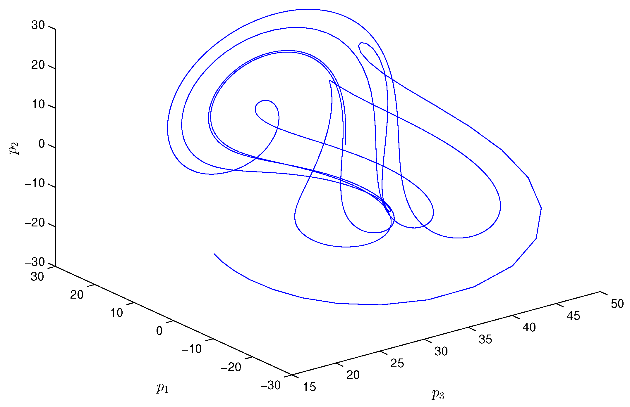
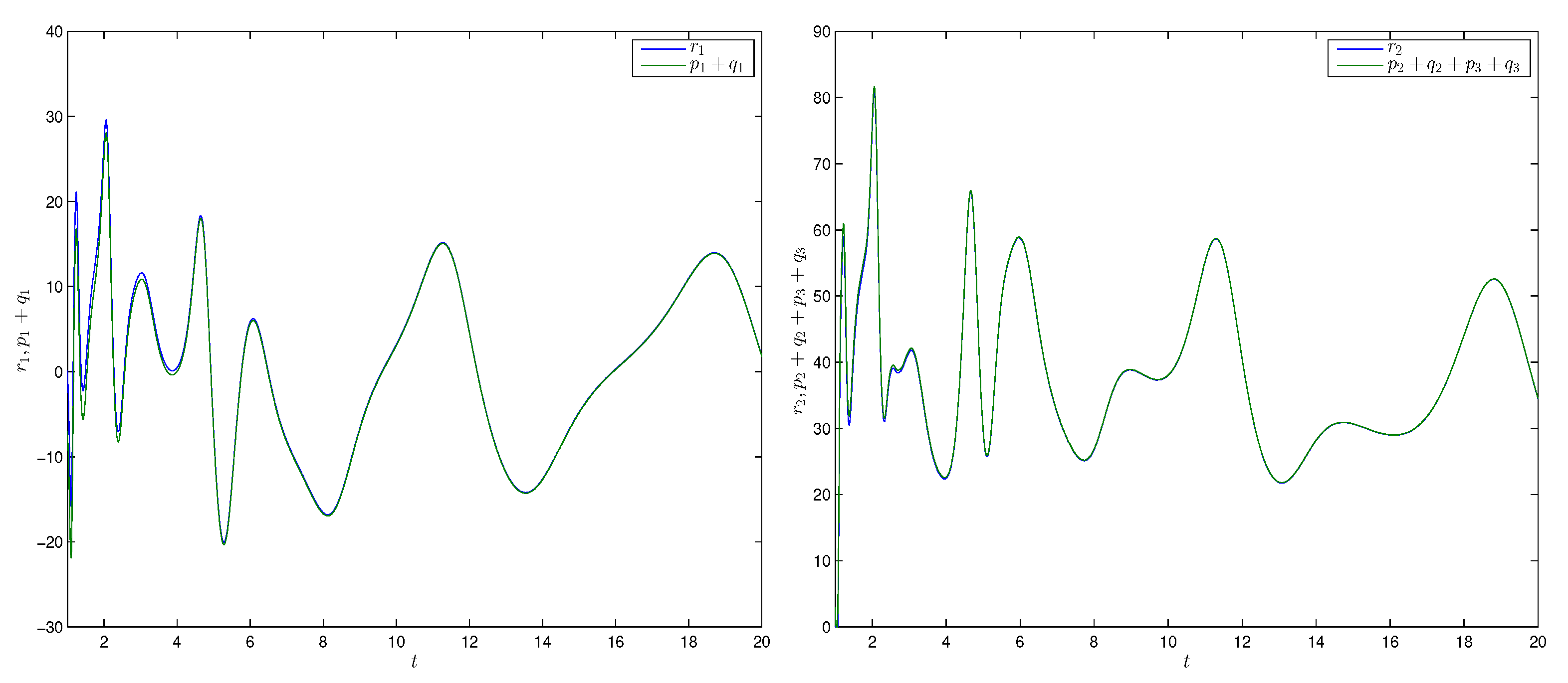
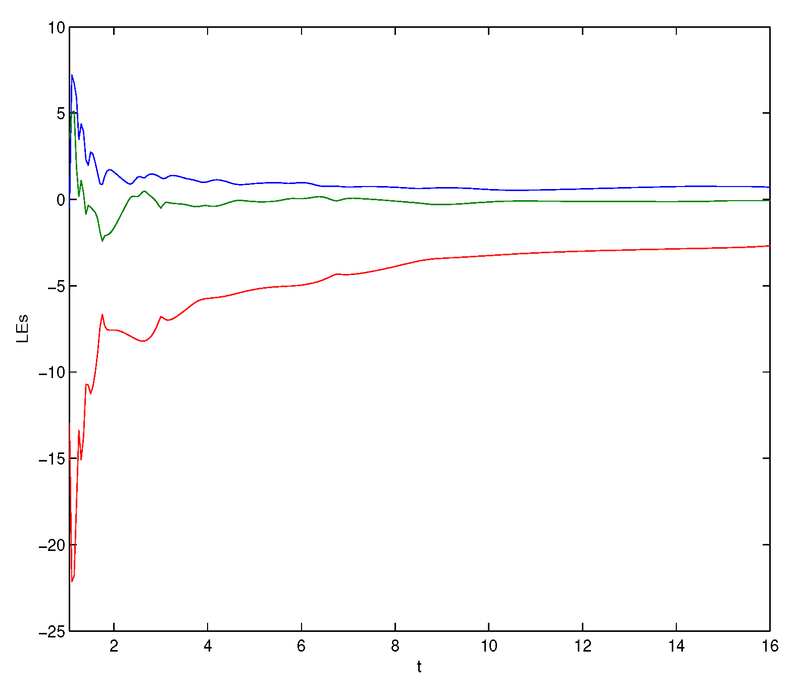
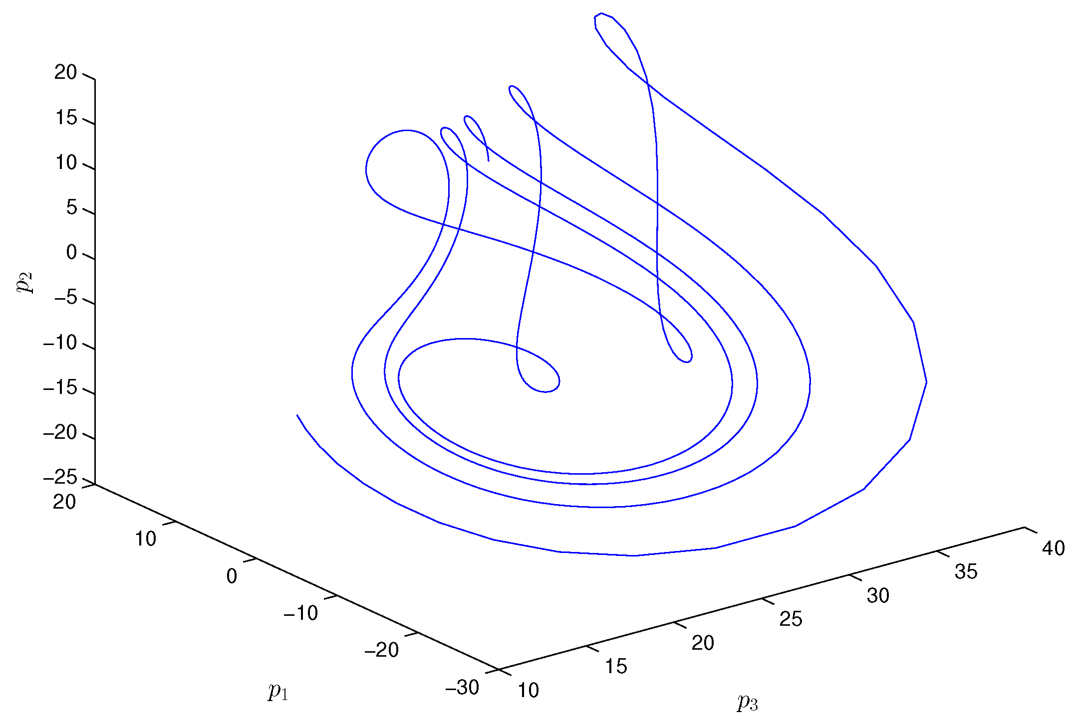
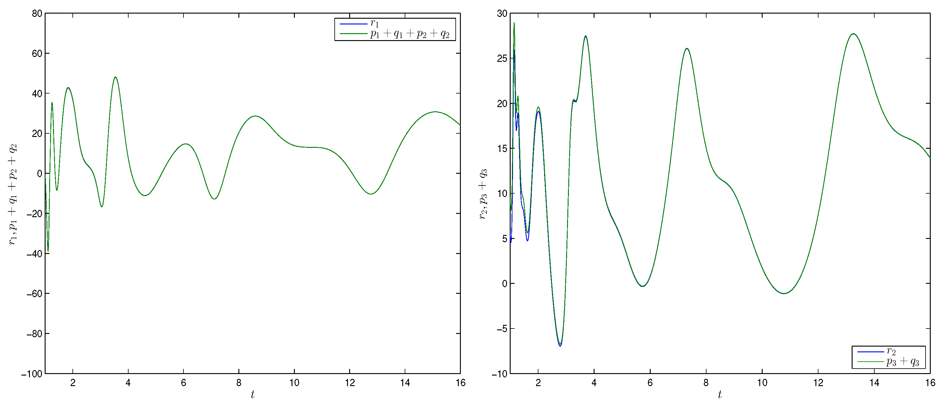
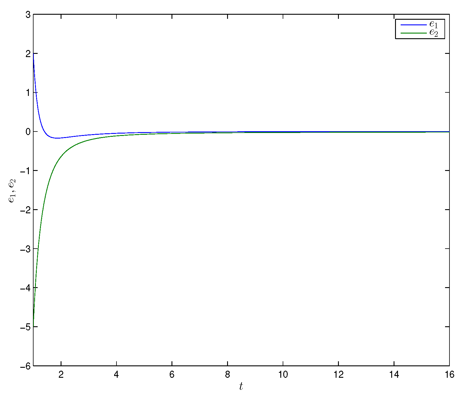
4. Numerical Simulations

In this section, numerical simulations for famous systems with Caputo–Hadamard derivatives were provided to clarify and verify the theoretical results obtained for the phenomenon of combination synchronization.

Example 1.

Let the first drive system be the non-autonomous Chen system with the Caputo–Hadamard derivative [29] as shown:

$$\begin{array}{ccc}{}^{CH}{\mathcal{D}}_{1,t}^{\varsigma }{p}_1\left(t\right)& =& (35+sin\left(t\right))(p_2-p_1)\\ {}^{CH}{\mathcal{D}}_{1,t}^{\varsigma }{p}_2\left(t\right)& =& 28p_2-p_1{p}_3\\ {}^{CH}{\mathcal{D}}_{1,t}^{\varsigma }{p}_3\left(t\right)& =& -3p_3+p_1{p}_2\end{array}.$$

(18)

According to Equation (1), we had:

$$R\left(t\right)=\left[\begin{array}{ccc}-(35+sin(t\left)\right)& 35+sin\left(t\right)& 0\\ 0& 28& 0\\ 0& 0& -3\end{array}\right],\mathbf{f}\left(\mathbf{p}\left(t\right)\right)=\left[\begin{array}{c}0\\ -p_1{p}_3\\ p_1{p}_2\end{array}\right].$$

The second drive system was taken as the non-autonomous fractional-order Lorenz system [30]:

$$\begin{array}{ccc}{}^{CH}{\mathcal{D}}_{1,t}^{\varsigma }{q}_1\left(t\right)& =& -2(q_1-q_2)\\ {}^{CH}{\mathcal{D}}_{1,t}^{\varsigma }{q}_2\left(t\right)& =& 10q_1-{sin}^2\left(2\pi t\right)q_2-q_1{q}_3\\ {}^{CH}{\mathcal{D}}_{1,t}^{\varsigma }{q}_3\left(t\right)& =& -{sin}^2\left(2{\pi }^{2}t\right)q_3+q_1{q}_2-10\end{array}.$$

(19)

System (19) could be expressed as system (2), where:

$$S\left(t\right)=\left[\begin{array}{ccc}-2& 2& 0\\ 10& -{sin}^2\left(2\pi t\right)& 0\\ 0& 0& -{sin}^2\left(2{\pi }^{2}t\right)\end{array}\right],\mathbf{g}\left(\mathbf{q}\left(t\right)\right)=\left[\begin{array}{c}0\\ -q_1{q}_3\\ q_1{q}_2-10\end{array}\right].$$

Now, we considered the response system as a nonlinear fractional-order Duffing system [31]:

$$\begin{array}{ccc}{}^{CH}{\mathcal{D}}_{1,t}^{\varsigma }{r}_1\left(t\right)& =& r_2+v_1\\ {}^{CH}{\mathcal{D}}_{1,t}^{\varsigma }{r}_2\left(t\right)& =& (0.5sin\left(t\right)+1)r_1-1.2r_2-r_1^3+v_2\end{array}.$$

(20)

System (20) could be written in equivalent form (3), by defining $T\left(t\right)$ and $\mathbf{h}\left(\mathbf{r}\right(t\left)\right)$, respectively, as:

$$T\left(t\right)=\left[\begin{array}{cc}0& 1\\ 0.5sin\left(t\right)+1& -1.2\end{array}\right],\mathbf{h}\left(\mathbf{r}\left(t\right)\right)=\left[\begin{array}{c}0\\ -r_1^3\end{array}\right].$$

If we chose the scaling matrix $M$ and the feedback gain matrix $N\left(t\right)$ as follows:

$$M=\left[\begin{array}{ccc}1& 0& 0\\ 0& 1& 1\end{array}\right],N\left(t\right)=\left[\begin{array}{cc}-2& -1+exp(-t)\\ -0.5sin\left(t\right)-1& -0.8\end{array}\right],$$

(21)

then, according to Equations (5) and (7), the components of the feedback control $\mathbf{v}\left(t\right)$ were given by:

$$\begin{array}{c}\hfill \begin{array}{cc}\hfill v_1\left(t\right)& =-2(q_1-q_2)+(35+sin\left(t\right))(p_2-p_1)-(q_2+p_2)-(q_3+p_3)\hfill \\ \hfill & -2(r_1-(q_1+p_1))+(-1+exp(-t))(r_2-(q_2+p_2+q_3+p_3)),\hfill \\ \hfill v_2\left(t\right)& =-q_1{q}_3+10q_1-{sin}^2\left(2\pi t\right)q_2-p_1{p}_3+28p_2+q_1{q}_2-{sin}^2\left(2{\pi }^{2}t\right)q_3\hfill \\ \hfill & -10+p_1{p}_2-3p_3-(0.5sin\left(t\right)+1)(q_1+p_1)+1.2(q_2+p_2+q_3+p_3)\hfill \\ \hfill & +r_1^3+(-0.5sin\left(t\right)-1)(r_1-(q_1+p_1))-0.8(r_2-(q_2+p_2+q_3+p_3)).\hfill \end{array}\end{array}$$

Based on the knowledge of the matrices $T\left(t\right)$ and $N\left(t\right)$, the combination synchronization error system became:

$${}^{CH}{\mathcal{D}}_{1,t}^{\varsigma }\mathbf{e}\left(t\right)=(T\left(t\right)+N\left(t\right))\mathbf{e}\left(t\right)=\left[\begin{array}{cc}-2& exp(-t)\\ 0& -2\end{array}\right]\mathbf{e}\left(t\right),$$

(22)

and

$$\underset{t\to \infty }{lim}(T\left(t\right)+N\left(t\right))=\left[\begin{array}{cc}-2& 0\\ 0& -2\end{array}\right]=T+N,$$

(23)

and this led to ${\displaystyle \underset{t\to +\infty }{lim}B\left(t\right)=0.}$ Moreover, since the eigenvalues of $A=T+N,$ were ${\mu }_1=-2$ and ${\mu }_2=-2,$ this implied that the condition of the spectrum of matrix $A$ satisfied. Thus, all hypotheses of Theorem 2 were achieved, and we could deduce that the combination synchronization phenomena were satisfied.

To obtain the numerical simulations, we used the modified predictor–corrector method [32]. Moreover, to investigate the chaos phenomenon of the system (18), we modified the MATLAB code proposed by Danca et al. [33], and this phenomenon could be identified by calculating the Lyapunov exponents (LEs). The corresponding Lyapunov exponents of system (18) were $0.3640,-0.0773,$ and $-2.0712.$ Figure 1 depicts the dynamics Lyapunov exponents, which showed that the first Lyapunov exponent was positive. This implied that the Chen system (18) was a chaotic system. Figure 2 displays the chaos of system (18) at $\varsigma =0.98$ and the initial condition $(-8,-10,16).$ The initial conditions of drive system (18) and the response system (20) were taken as $(1,2,-5)$, and $(0.1,0.2),$ respectively. In addition, the corresponding initial condition of the error system was given by $(-2.5,-5.5).$

Figure 3 shows the time trajectories of states $r_1\left(t\right),p_1\left(t\right)+q_1\left(t\right)$ and $r_2\left(t\right),p_2\left(t\right)+q_2\left(t\right)+p_3\left(t\right)+q_3\left(t\right),$ of the two derive systems (18) (19) and a response system (20), respectively, which implied that the two derive systems (18), (19) would attain combination synchronization with response system (20). The combination synchronization error is shown in Figure 4. From the numerical simulations given in Figure 3 and Figure 4, it was remarkable that the theoretical results were satisfied.

Example 2.

In this example, the Chen system [34] and the Lorenz system [35] with Caputo–Hadamard derivatives were used as the drive systems, while we considered the modified Van der Pol equation [36] with the Caputo–Hadamard derivative as the response system. The Chen and Lorenz systems with Caputo–Hadamard derivatives were given, respectively, by:

$${}^{CH}{\mathcal{D}}_{1,t}^{\varsigma }\mathbf{p}\left(t\right)=\underset{R\left(t\right)}{\underbrace{\left[\begin{array}{ccc}-\alpha & \alpha & 0\\ \gamma -\alpha & \gamma & 0\\ 0& 0& -\beta \end{array}\right]}}\mathbf{p}\left(t\right)+\underset{\mathbf{f}\left(\mathbf{p}\right(t\left)\right)}{\underbrace{\left[\begin{array}{c}0\\ -p_1{p}_3\\ p_1{p}_2\end{array}\right]}},$$

(24)

$${}^{CH}{\mathcal{D}}_{1,t}^{\varsigma }\mathbf{q}\left(t\right)=\underset{S\left(t\right)}{\underbrace{\left[\begin{array}{ccc}-\zeta & \zeta & 0\\ -\zeta & -1& 0\\ 0& 0& -\eta \end{array}\right]}}\mathbf{q}\left(t\right)+\underset{\mathbf{g}\left(\mathbf{q}\right(t\left)\right)}{\underbrace{\left[\begin{array}{c}0\\ -q_1{q}_3\\ q_1{q}_2-\eta (\zeta +\rho )\end{array}\right]}},$$

(25)

where $\mathbf{p}\left(t\right)={[p_1\left(t\right),p_2\left(t\right),p_3\left(t\right)]}^T$, $\mathbf{q}\left(t\right)={[q_1\left(t\right),q_2\left(t\right),q_3\left(t\right)]}^T,$$t>t_0>0,0<\varsigma \le 1$ and $\alpha ,\beta ,\gamma ,\zeta ,\eta ,$ and ρ are real parameters. The modified Van der Pol equation with the Caputo–Hadamard derivative was presented as:

$${}^{CH}{\mathcal{D}}_{1,t}^{\varsigma }\mathbf{r}\left(t\right)=\underset{T\left(t\right)}{\underbrace{\left[\begin{array}{cc}0& 1\\ 0& \sigma \end{array}\right]}}\mathbf{r}\left(t\right)+\underset{\mathbf{h}\left(\mathbf{r}\right(t\left)\right)}{\underbrace{\left[\begin{array}{c}0\\ -\sigma r_1^2{r}_2-r_1^3+bcos\left(t\right)\end{array}\right]}}+\mathbf{v}\left(t\right),$$

(26)

where $\mathbf{r}\left(t\right)={[r_1\left(t\right),r_2\left(t\right)]}^T$, $\mathbf{v}\left(t\right)={[v_1\left(t\right),v_2\left(t\right)]}^T,$σ and b were positive constants.

Now, if we chose matrices $M$ and $N\left(t\right)$ as:

$$M=\left[\begin{array}{ccc}1& 1& 0\\ 0& 0& 1\end{array}\right],N\left(t\right)=\left[\begin{array}{cc}-4& 0\\ 0& \mu -3\end{array}\right],$$

then the components of the feedback control were provided by:

$$\begin{array}{c}\hfill \begin{array}{cc}\hfill v_1\left(t\right)& =-\zeta q_1+\zeta q_2-\alpha p_1+\alpha p_2-\zeta q_1-q_2-q_1{q}_3+(\gamma -\alpha )p_1\hfill \\ \hfill & +\gamma p_2-p_1{p}_3-(p_3+p_3)-4(r_1-(p_1+q_1+p_2+q_2)),\hfill \\ \hfill v_2\left(t\right)& =-\eta q_3+q_1{q}_2-\eta (\zeta +\rho )-\beta p_3+p_1{p}_2-\mu (p_3+q_3)+\mu r_1^2{r}_2\hfill \\ \hfill & +r_1^3-bcos\left(t\right)-(\sigma +3)(r_2-(p_3+q_3)),\hfill \end{array}\end{array}$$

and we could obtain the combination synchronization error system by:

$${}^{CH}{\mathcal{D}}_{1,t}^{\varsigma }\mathbf{e}\left(t\right)=(T\left(t\right)+N\left(t\right))\mathbf{e}\left(t\right)=\left[\begin{array}{cc}-4& 1\\ 0& -3\end{array}\right]\mathbf{e}\left(t\right).$$

To verify Theorem 2, one could compute that:

$$\underset{t\to \infty }{lim}(T\left(t\right)+N\left(t\right))=\left[\begin{array}{cc}-4& 1\\ 0& -3\end{array}\right]=T+N,$$

and this led to ${\displaystyle \underset{t\to +\infty }{lim}B\left(t\right)=0.}$ Furthermore, the corresponding eigenvalues of $A=T+N,$ were given by ${\mu }_1=-4$ and ${\mu }_2=-3,$ which implied that $|arg\mu |>\frac{\varsigma \pi }{2}$ satisfied. Therefore, the combination synchronization phenomena were achieved.

In the numerical simulations, the parameter values of the fractional-order Chen system, Lorenz system, and modified Van der Pol system were given as $(\alpha ,\beta ,\gamma )=(35,3,28)$, $(\zeta ,\eta ,\rho )=(10,8/3,28)$ and $(\sigma ,b)=(1,1)$, respectively. The initial states of the two drive systems and response system were arbitrarily chosen as $(-5,-7,10)$, $(5.5,5.5,-0.5)$, and $(0,5.5)$, respectively. Moreover, the initial state of the error vector was $(2,-5).$ The dynamics of Lyapunov exponents of system (24) are shown in Figure 5, where the corresponding LEs were $0.7113-0.0675,$ and $-2.6904.$ Accordingly, it was obvious that the Chen system (24) was chaotic.

Figure 6 elucidates the chaotic behavior of system (24) at the given chosen parameters and $\varsigma =0.98.$ Figure 7 exhibits the identicality of the time trajectories of the states $r_1\left(t\right),p_1\left(t\right)+q_1\left(t\right)+p_2\left(t\right)+q_2\left(t\right)$ and $r_2\left(t\right),p_3\left(t\right)+q_3\left(t\right)$. Furthermore, Figure 8 displays the error dynamics for the systems presented in Example 2. It was clear that the numerical results shown in all Figures confirmed the theoretical results.

5. Conclusions

In this paper, combination synchronization phenomena of several fractional-order systems employing the scaling matrix were discussed. To the best of our knowledge, the proposed synchronization for fractional-order systems involving the Caputo–Hadamard derivative has not been previously investigated. Combination synchronization was accomplished by taking into account two drive systems and one response system. We demonstrated that the phenomenon of combination synchronization could be achieved theoretically. In addition, numerical simulations were performed to demonstrate the feasibility and validity of the given theoretical analysis. Finally, the presented results pave the way for future research not only into various types of combination synchronization, such as using linear control, adaptive control, and active control, but also into investigating the possibility of extending the proposed synchronization to other fractional-order derivatives. Furthermore, in future work, we will investigate whether the proposed synchronization technique can be applied to a class of different fractional-order systems with unequal orders.

References

1. Hilfer, R. Applications of Fractional Calculus in Physics; World Scientific: Singapore, 2000. [Google Scholar]
2. Podlubny, I. Fractional Differential Equations; Academic Press: New York, NY, USA, 1999. [Google Scholar]
3. Ahmadova, A.; Mahmudov, N.I. Langevin differential equations with general fractional orders and their applications to electric circuit theory. J. Comput. Appl. Math. 2021, 388, 113299. [Google Scholar] [CrossRef]
4. Patel, V.K.; Bahuguna, D. An efficient matrix approach for the numerical solutions of electromagnetic wave model based on fractional partial derivative. Appl. Numer. Math. 2021, 169, 1–20. [Google Scholar] [CrossRef]
5. Sunarto, A.; Agarwal, P.; Sulaiman, J.; Chew, J.V.L.; Aruchunan, E. Iterative method for solving one-dimensional fractional mathematical physics model via quarter-sweep and PAOR. Adv. Differ. Equ. 2021, 2021, 147. [Google Scholar] [CrossRef]
6. Tassaddiq, A.; Khan, I.; Nisar, K.S.; Singh, J. MHD flow of a generalized Casson fluid with Newtonian heating: A fractional model with Mittag–Leffler memory. Alex. Eng. J. 2020, 59, 3049–3059. [Google Scholar] [CrossRef]
7. Xi, H.; Lia, Y.; Huanga, X. Adaptive function projective combination synchronization of three different fractional-order chaotic systems. Optik 2015, 126, 5346–5349. [Google Scholar] [CrossRef]
8. Kilbas, A.A.; Srivastava, H.M.; Trujillo, J.J. Theory and Applications of Fractional Differential Equations; Elsevier: Amsterdam, Switzerland, 2006. [Google Scholar]
9. Katugampola, U.N. A new approach to generalized fractional derivative. Bull. Math. Anal. Appl. 2014, 6, 1–15. [Google Scholar]
10. Adjabi, Y.; Jarad, F.; Baleanu, D.; Abdeljawad, T. On Cauchy problems with Caputo Hadamard fractional derivatives. J. Comput. Anal. Appl. 2016, 21, 661–681. [Google Scholar]
11. Jarad, F.; Abdeljawad, T.; Baleanu, D. Caputo-type modification of the Hadamard fractional derivatives. Adv. Differ. Equ. 2012, 2012, 142. [Google Scholar] [CrossRef] [Green Version]
12. Nain, A.; Vats, R.; Kumar, A. Coupled fractional differential equations involving Caputo-Hadamard derivative with nonlocal boundary conditions. Math. Meth. Appl. Sci. 2021, 44, 4192–4204. [Google Scholar] [CrossRef]
13. Amara, A.; Etemad, S.; Rezapour, S. Topological degree theory and Caputo–Hadamard fractional boundary value problems. Adv. Differ. Equ. 2020, 2020, 369. [Google Scholar] [CrossRef]
14. Etemad, S.; Rezapour, S.; Samei, M.E. On a fractional Caputo–Hadamard inclusion problem with sum boundary value conditions by using approximate endpoint property. Math Meth Appl Sci. 2020, 43, 9719–9734. [Google Scholar] [CrossRef]
15. Pecora, L.M.; Carroll, T.L. Synchronization in chaotic systems. Phys. Rev. Lett. 1990, 64, 821–824. [Google Scholar] [CrossRef] [PubMed]
16. Chen, J.; Jiao, L.; Wu, J.; Wang, X. Projective synchronization with different scale factors in driven-response complex network and its application to image encryption. Nonlinear Anal. 2010, 11, 3045–3058. [Google Scholar] [CrossRef]
17. Hong-Yan, Z.; Le-Quan, M.; Geng, Z.; Guan-Rong, C. Generalized chaos synchronization of bidirectional arrays of discrete systems. Chin. Phys. Lett. 2013, 30, 040502. [Google Scholar]
18. Kareem, S.O.; Ojo, K.S.; Njah, A.N. Function projective synchronization of identical and non-identical modified finance and Shimizu-Morioka systems. Pramana 2012, 79, 71–79. [Google Scholar] [CrossRef]
19. Li, G.H. Modified projective synchronization of chaotic system. Chaos Solitons Fractals 2007, 32, 1786–1790. [Google Scholar] [CrossRef]
20. Runiz, L.; Zhengmin, W. Adaptive function projective synchronization of unified chaotic systems with uncertain parameters. Chaos Solitons Fractals 2009, 42, 1266–1272. [Google Scholar] [CrossRef]
21. Runzi, L.; Yinglan, W.; Shucheng, D. Combination synchronization of three classic chaotic systems using active backstepping design. Chaos Interdiscip. J. Nonlinear Sci. 2011, 21, 043114. [Google Scholar] [CrossRef]
22. Vincent, U.E.; Saseyi, A.O.; McClintock, P.V. Multiswitching combination synchronization of chaotic systems. Nonlinear Dyn. 2015, 80, 845–854. [Google Scholar] [CrossRef] [Green Version]
23. Wang, S.B.; Wang, X.Y.; Wang, X.Y.; Zhou, Y.F. Adaptive generalized combination complex synchronization of uncertain real and complex nonlinear systems. AIP Adv. 2016, 6, 045011. [Google Scholar] [CrossRef] [Green Version]
24. Singh, A.K.; Vijay, K.Y.; Das, S. Dual combination synchronization of the fractional order complex chaotic systems. J. Comput. Nonlinear Dyn. 2017, 12, 011017. [Google Scholar] [CrossRef]
25. Vijay, K.Y.; Prasad, G.; Srivastava, M.; Das, S. Combinationcombination phase synchronization among non-identical fractional order complex chaotic systems via nonlinear control. Int. J. Dynam. Control 2018, 7, 330–340. [Google Scholar]
26. Zerimeche, H.; Houmor, T.; Berkane, A. Combination synchronization of different dimensions fractional-order non-autonomous chaotic systems using scaling matrix. Int. J. Dyn. Control 2021, 9, 788–796. [Google Scholar] [CrossRef]
27. Almeida, R. Caputo–Hadamard fractional derivatives of variable order. Numer. Funct. Anal. Optim. 2017, 38, 1–19. [Google Scholar] [CrossRef] [Green Version]
28. Cong, N.D.; Doan, T.S.; Tuan, H.T. Asymptotic stability of linear fractional systems with constant coefficients and small time dependent perturbations. Vietnam. J. Math. 2018, 46, 665–680. [Google Scholar] [CrossRef] [Green Version]
29. Huang, S.; Zhang, R.; Chen, D. Stability of nonlinear fractionalorder time varying systems. ASME J. Comput. Nonlinear Dyn. 2016, 11, 031007. [Google Scholar] [CrossRef]
30. Xu, Z. Dynamics of a class of fractional-order nonautonomous Lorenz-type systems. Chaos 2017, 27, 041104. [Google Scholar]
31. Lei, Y.; Xu, W.; Xu, Y.; Fang, T. Chaos control by harmonic excitation with propoer random phase. Chaos Solitons Fractals 2004, 21, 1175–1181. [Google Scholar] [CrossRef]
32. Gohar, M.; Li, C.; Li, Z. Finite difference methods for caputo–hadamard fractional differential equations. Mediterr. J. Math. 2020, 17, 194. [Google Scholar] [CrossRef]
33. Danca, M.F.; Kuznetsov, N. Matlab Code for Lyapunov Exponents of Fractional-Order Systems. Int. J. Bifurc. Chaos 2018, 25, 1850067. [Google Scholar] [CrossRef] [Green Version]
34. Chen, G.R.; Ueta, T. Yet another chaotic attractor. Int. J. Bifurc. Chaos 1999, 9, 1465–1466. [Google Scholar] [CrossRef]
35. Hayden, K.; Olson, E.; Titi, E.S. Discrete data assimilation in the Lorenz and 2D Navier–Stokes equations. Phys. D 2011, 240, 1416–1425. [Google Scholar] [CrossRef] [Green Version]
36. Ku, Y.H.; Sun, X. Chaos in Van der Pol’s equation. J. Franklin Inst. 1990, 327, 197–207. [Google Scholar] [CrossRef]
Figure 1. Lyapunov exponent dynamics from a Chen system (18).
Mathematics 09 02781 g001
Figure 2. A 3D phase portrait of the non-autonomous Chen system (18).
Mathematics 09 02781 g002
Figure 3. Time trajectories of states r 1 ( t ) , p 1 ( t ) + q 1 ( t ) and r 2 ( t ) , p 2 ( t ) + q 2 ( t ) + p 3 ( t ) + q 3 ( t ) , for Example 1.
Mathematics 09 02781 g003
Figure 4. Error dynamics between the drive systems and the response system for Example 1.
Mathematics 09 02781 g004
Figure 5. Lyapunov exponent dynamics from a Chen system (24).
Mathematics 09 02781 g005
Figure 6. A 3D phase portrait of the Chen system (24).
Mathematics 09 02781 g006
Figure 7. Time trajectories of states r 1 ( t ) , p 1 ( t ) + q 1 ( t ) + p 2 ( t ) + q 2 ( t ) and r 2 ( t ) , p 3 ( t ) + q 3 ( t ) , for Example 2.
Mathematics 09 02781 g007
Figure 8. Error dynamics between the drive systems and the response system for Example 2.
Mathematics 09 02781 g008
Publisher’s Note: MDPI stays neutral with regard to jurisdictional claims in published maps and institutional affiliations.