Observation of a Change in Human Attitude in a Decision Making Process Equipped with an Interference of a Third Party

Abstract

In this paper, the attitudes of experts are observed for the possible changes after taking a certain decision. The decision is taken by two persons with different fields of expertise. There is also an annotation of such changes due to the interference of a third person, which is main idea of this paper. These observations are done by developing fuzzy soft differential equations with the help of optimum fuzzy soft constants (OFSCs), which are obtained through the ranking coefficients. The ranking of alternatives is based on the coefficients, which are obtained through a decision-making process. Technique for Order of Preference by Similarity to Ideal Solution (TOPSIS) is exploited to rank the alternatives, and the attitudes of resource persons are examined through phase portraits and line graphs of the respective system of differential equations. The utilization of TOPSIS is a practice of multi-criteria decision-making in the analysis of human behaviours. Dual hesitant fuzzy soft sets are taken to represent the initial data.

1. Introduction

A concept of a hesitant fuzzy set (HFS) [1] plays a vital role to handle the situations where assigning a single value from [0, 1] to an element becomes difficult. HFS theory can be viewed as an extension of a fuzzy set theory and has attracted the attention of many researchers due to its applications in social sciences and artificial intelligence. Torra [2] studied some basic operations on such sets. To rank the hesitant fuzzy elements (HFEs), score functions are defined. Wang et al. [3] studied a special characteristic of score functions. Some useful information measures for HFSs were studied by Farhadinia [4]. A variety of distance and similarity measures were investigated by Xu and Xia (2011). They also presented ordered distance and ordered similarity measures. Distance and similarity measures have considerable importance in many scientific fields such as decision making, pattern recognition, machine learning and market prediction. Wang et al. [5] studied HFSs in the framework of a soft set theory and introduced the concept of hesitant fuzzy soft sets (HFSSs). In this way, they extended the notion of a classical soft set to hesitant fuzzy soft set. They first defined the operations of complement, “AND”, “OR”, union and intersection on HFSS, then proved De-Morgan Laws. Peng and Yang [6] proposed the concept of interval-valued hesitant fuzzy soft set (IVHFSS) which is the combination of the interval-valued hesitant fuzzy set and soft set. They also defined the basic operations and geometric operations on the IVHFSS. Intuitionistic fuzzy set theory [7] is used to describe the degree of membership as well as non-membership simultaneously. Grzegorzewski [8] defined the distances between intuitionistic fuzzy sets. Dual hesitant fuzzy set (DHFS) [9] encircles intuitionistic fuzzy set and hesitant fuzzy set. Zhu et al. [9] defined some basic operations on DHFS and then score function and accuracy function for dual hesitant fuzzy elements. Singh [10] presented the distance and similarity measures for DHFS. Dual hesitant fuzzy soft set (DHFSS) was defined by Zhang and Shu [11]. Garg and Arora [12] defined the distance and similarity measures for DHFSS. They also presented some relations satisfied by different distance measures and found an application of such measures in pattern recognition.

Decision making is one of the unavoidable human needs in the daily life of business. Different decision making techniques are applied when some criteria/attributes or limitations are given. In such techniques, different weights are obtained from the group of experts for different criteria. Aruldoss et al. [13] proposed the methods for multi-criteria decision making (MCDM). They presented a comparison of contributions of MCDM methods. It can be seen that TOPSIS (Technique for Order of Preference by Similarity to Ideal Solution) has a remarkable contribution in multi-criteria decision making. Many researchers [6,14,15,16,17,18] used TOPSIS to solve problems arising in various decision making processes based on fuzzy soft set, intuitionistic fuzzy soft set and hesitant fuzzy soft set theories. This method has an aspect that the solution should be close to the perfect situation and far from the poor situation. Wang et al. [19] employed TOPSIS in the setup of dual hesitant fuzzy set theory. Recently, some MCDM methods have been presented with different applications [20,21].

Uncertainty in dynamic systems is modelled by using fuzzy differential equations (FDEs) [22]. Puri and Ralescu [23] defined differentials of a fuzzy function. Kaleva ([24]) studied differentiability and integrability properties of fuzzy set-valued mappings and gave an existence and uniqueness theorem for a solution to a FDE. Buckley and Feuring [25] presented a solution to the fuzzy first order initial value problem. A lot of practical problems can be modelled as FDEs [26] and can be solved by replacing with system of differential equations [27]. Beg et al. [28] developed a system of differential equations to study the behaviour of some individual over the time depending on their companion’s attitude under some particular situation. They used optimum fuzzy soft constant (OFSC) to model the system of differential equations. Strogatz [29] discussed the stability of such types of systems. This system of differential equations was also constructed by Sprott [30] to investigate the future behaviour of Romeo and Juliet in their love affair. He also extended that system when there is an interference of a third person in their affair. This interference may change their initial opinions or their interpersonal influences. Interpersonal influences are represented in matrix form and play a key role in influence models [31,32].

This paper is motivated by the dynamic model presented by Sprott [30]. After that, there has been a gap of the study related to the interferences in the field of decision making except [33,34]. This paper consists of the observation of the influence of a third person after a decision had been taken by two persons. For this purpose, a system of differential equations is developed with fuzzy initial conditions (FICs) and OFSCs are obtained from the coefficients of relative closeness. These coefficients are calculated by using TOPSIS due to its suitability while initial data is taken as dual hesitant fuzzy soft set since it includes multi-values for both membership and non-membership degrees. An illustrative example is given to understand the proposed idea.

2. Preliminaries

Throughout this paper, X denotes a non-empty set of objects.

Definition 1

([2]). Hesitant fuzzy set (HFS) M on X can be characterized as: $M=\left\{〈x,h_M\left(x\right)〉\mid x\in X\right\}$ where $h_M\left(x\right)$ is a subset of $\left[0,1\right]$, representing the possible membership degrees of an element $x\in X$ to the set M.

In the sequel, by hesitant fuzzy set, we mean a discrete hesitant fuzzy set where each $h_A\left(x\right)$ is a finite set in $\left[0,1\right]$.

Definition 2

([7]). An intuitionistic fuzzy set (IFS) I on X is an object having the form $I=\left\{〈x,{\mu }_I\left(x\right),{\nu }_I\left(x\right)〉\mid x\in X\right\}$, that is, an intuitionistic fuzzy set (IFS) I on X is characterized by a membership function ${\mu }_I$ and a non-membership function ${\nu }_I$, where ${\mu }_I:X⟶\left[0,1\right]$ and ${\nu }_I:X⟶\left[0,1\right]$, satisfying the condition $0\le$${\mu }_I\left(x\right) + {\nu }_I\left(x\right)\le 1,$ $\forall x\in X.$

Definition 3

([9]). A dual hesitant fuzzy set (DHFS) D on X is represented by the set $D=\left\{〈x,h_D\left(x\right),g_D\left(x\right)〉\mid x\in X\right\}$, where $h_D\left(x\right)$ and $g_D\left(x\right)$ are two sets having some values in $\left[0,1\right]$ representing the possible membership degrees and non-membership degrees of the element $x\in X$, respectively, satisfying the conditions: $0\le \mu , \nu \le 1,$$0\le {\mu }^{+}+{\nu }^{+}\le 1$ where $\mu \in h_D\left(x\right),$$\nu \in g_D\left(x\right),$${\mu }^{+}\in h_D^{+}\left(x\right)={\cup }_{\mu \in h_D\left(x\right)}max\left\{\mu \right\},$${\nu }^{+}\in g_D^{+}\left(x\right)={\cup }_{\nu \in g_D\left(x\right)}max\left\{\nu \right\}$ for all $x\in X.$

If each $h_D\left(x\right)$ and $g_D\left(x\right)$ are finite sets, then D is known as a discrete dual hesitant fuzzy set (DDHFS).

Definition 4

([11]). Let $(X,E)$ be a soft universe and $P\subseteq E$. A pair $\left(\tilde{F},P\right)$ is called a dual hesitant fuzzy soft set (DHFSS) over X provided that $\tilde{F}$ is a mapping from P to the set of all DHF sets on X.

$\left(\tilde{F},P\right)$ is called a discrete dual hesitant fuzzy soft set (DDHFSS) over U if $\tilde{F}$ is a mapping from P to the set of all DDHF sets on U.

Definition 5

([19]). Let A and B be two $DHFSs$ on $X=\left\{x_1,x_2,\dots ,x_n\right\}$. Then, the distance between A and B is denoted by $d(A,B)$ and satisfies the following properties:

(1) 

$0\le d(A,B)\le 1;$

(2) 

$d(A,B)=0$ if and only if $A=B;$

(3) 

$d(A,B)=d(B,A).$

Definition 6

([19]). Let M and N be two $DHFSs$ on $X=\left\{x_1,x_2,\dots ,x_n\right\}$, then generalized dual hesitant normalized distance between the sets M and N is defined as:

$${\displaystyle d(M,N)=\sum _{i=1}^n{\left[\frac{1}{n}\left[\frac{1}{l_{x_i}}\left[\begin{array}{c}{\displaystyle \sum _{j=1}^{\#h_{x_i}}{\left|{\mu }_M^{\sigma \left(j\right)}\left(x_i\right)-{\mu }_N^{\sigma \left(j\right)}\left(x_i\right)\right|}^{\lambda }}\\ {\displaystyle +\sum _{k=1}^{\#g_{x_i}}{\left|{\nu }_M^{\sigma \left(k\right)}\left(x_i\right)-{\nu }_N^{\sigma \left(k\right)}\left(x_i\right)\right|}^{\lambda }}\end{array}\right]\right]\right]}^{\frac{1}{\lambda }},}$$

where $\lambda >0$, $l_{x_i}=\left(\#h_{x_i}\right)+\left(\#g_{x_i}\right)$, where $\#h$ and $\#g$ are the numbers of the elements in the sets given by h and g, respectively.

The above distance measure is the generalization of the distances given by Grzegorzewski [8] and Xu and Xia [35]. If $\lambda =1$, then the generalized dual hesitant normal distance becomes the dual hesitant normalized Hamming distance; if $\lambda =2$, then it reduces to the dual hesitant normalized Euclidean distance.

2.1. Fuzzy Numbers and Fuzzy Functions

Definition 7

([27]). A fuzzy number x is defined by a pair $x=(\underline{x},\overline{x})$ of functions $\underline{x},\overline{x}:[0,1]⟶R$, satisfying the three conditions:

1. 

$\underline{x}\left(\alpha \right)$ is a bounded, monotonically increasing left-continuous function for all $\alpha \in (0,1]$ and right-continuous for $\alpha =0$,

2. 

$\overline{x}\left(\alpha \right)$ is a bounded, monotonically decreasing left-continuous function for all $\alpha \in (0,1]$ and right-continuous for $\alpha =0$,

3. 

For all $\alpha \in (0,1]$ we have: $\underline{x}\le \overline{x}$.

Definition 8

([27]). Let $x=(\underline{x},\overline{x})$ and $y=(\underline{y},\overline{y})$ be two arbitrary numbers, then the distance between x and y is defined as follows:

$$d(x,y)=\underset{\alpha \in [0,1]}{sup}\{max[\mid \underline{x\left(\alpha \right)}-\underline{y\left(\alpha \right)}\mid ,\mid \overline{x\left(\alpha \right)}-\overline{y\left(\alpha \right)}\mid ]\}.$$

It can be proved that $(E^1,d)$ is a complete metric space [23].

Definition 9

([27]). A fuzzy function $g:R^1\to E^1$ is said to be continuous if for an arbitrary fixed $t_{\circ }\in R^1$ and $\epsilon >0$ there exists a $\delta >0$ such that:

$$|t-t_{\circ }|<\delta \Rightarrow d(g\left(t\right),g\left(\widehat{t}\right))<\epsilon ,$$

then g is said to be continuous.

Definition 10

([27]). Let $x,y\in E^1$. If there exists $z\in E^1$ such that $x=y+z$, then z is called the H-difference of $x,y$ and it is denoted by $x-y$.

Definition 11

([27]). A function $g:(c,d)\to E^1$ is said to be H-differentiable at $t_{\circ }\in (c,d)$ if for a small $h>0$, there exist the H-differences $g\left(t_{\circ }\right)-g(t_{\circ }-h)$, $g(t_{\circ }+h)-g\left(t_{\circ }\right)$ and the element $g^{\prime }\left(t_{\circ }\right)\in E^1$ such that:

$$0=\underset{h\to 0^{+}}{lim}d\left(\frac{g\left(t_{\circ }\right)-g(t_{\circ }-h)}{h},g^{\prime }\left(t_{\circ }\right)\right)=\underset{h\to 0^{+}}{lim}d\left(\frac{g(t_{\circ }+h)-g\left(t_{\circ }\right)}{h},g^{\prime }\left(t_{\circ }\right)\right),$$

then $g^{\prime }\left(t_{\circ }\right)$ is called the fuzzy derivative of g at $t_{\circ }$.

Definition 12

([36]). The triangular fuzzy numbers are common and are denoted by $x=(\alpha ,c,\beta )$ and defined by:

$$x=\left\{\begin{array}{cc}\frac{u-\alpha }{c-\alpha },\hfill & \mathit{if}\alpha \le u\le c,\hfill \\ \frac{\beta -u}{\beta -c},\hfill & \mathit{if}c\le u\le \beta ,\hfill \\ 0,\hfill & \mathit{otherwise}.\hfill \end{array}\right.$$

2.2. First Order Fuzzy Differential Equation

A first order fuzzy differential equation is written in the following form:

$$x^{\prime }\left(t\right)=f(t,x\left(t\right))$$

where x is a fuzzy function of t and $f(t,x)$ is a fuzzy function of the crisp variable t and the fuzzy variable x. Here, $x^{\prime }$ is the fuzzy derivative of x. Consider the initial value problem

$$\begin{array}{ccc}{x}^{\prime }\left(t\right)=f(t,x\left(t\right)),& & x\left(t_{\circ }\right)=x_{\circ }\end{array}$$

(1)

A mapping $x:R^1\to E^1$ is a solution to the problem (1) if and only if it is continuous and satisfies the integral equation

$$x\left(t\right)=x_{\circ }+{\int }_{t_{\circ }}^{t}f(s,x\left(s\right))ds$$

for all $t\in R^1$ [24].

To obtain the solution of Equation (1), it can be replaced by the following equivalent system:

$$\begin{array}{ccc}{\underline{x}}^{\prime }\left(t\right)=\underline{f}(t,x\left(t\right)),& & \underline{x}\left(t_{\circ }\right)=\underline{x_{\circ }},\\ {\overline{x}}^{\prime }\left(t\right)=\overline{f}(t,x\left(t\right)),& & \overline{x}\left(t_{\circ }\right)=\overline{x_{\circ }}.\end{array}$$

For example, to solve

$$\begin{array}{ccc}\frac{dx}{dt}=t^{2}x& ,& x\left(0\right)=(0,\frac{1}{2},1),\end{array}$$

(initial condition is represented in Figure 1).

It is replaced by

$$\begin{array}{cc}\frac{d\underline{x}}{dt}=t^2\underline{x},& \underline{x}\left(0\right)=(0,\frac{1}{2}),\\ \frac{d\overline{x}}{dt}=t^2\overline{x},& \overline{x}\left(0\right)=(\frac{1}{2},1),\end{array}$$

$\underline{x}\left(0\right)=(0,\frac{1}{2})$ and $\overline{x}\left(0\right)=(\frac{1}{2},1)$ are replaced by parametric forms $\underline{x}\left(0\right)=2r$ and $\overline{x}\left(0\right)=2(1-r)$, respectively, where $r\in [0,1]$. Furthermore, the solution is:

$$\begin{array}{c}x=(2r{e}^{\frac{t^3}{3}},2(1-r)e^{\frac{t^3}{3}}),\&r\in [0,1],\end{array}$$

which is represented in Figure 2.

2.3. Fuzzy Soft Differential Equations

To analyse the human attitude: a system of linear fuzzy soft differential equations is designed in two variables, namely P₁ and P₂ which represent the attitude of two persons at the time t of decision making, whereas $\frac{d{P}_1}{dt}$ and $\frac{d{P}_2}{dt}$ denote the change in persons’ attitudes after some time due to the decision they made (Beg et al., 2018).

$$\begin{array}{c}\frac{d{P}_1}{dt}=a_{P_1}^1{P}_1+a_{P_2}^1{P}_2\\ \frac{d{P}_2}{dt}=a_{P_1}^2{P}_1+a_{P_2}^2{P}_2\end{array}$$

(2)

where $a_{P_j}^i$$(i,j=1,2)$ are signed fuzzy numbers called optimum soft fuzzy constants. We may interpret $a_{P_i}^i$ as the influence on $ith$ person of their internal feelings and $a_{P_j}^i$ the influence on $ith$ person of $jth$ person’s feelings. Positive and negative sign is assigned to $a_{P_j}^i$ based on encouragement or discouragement of a person about a decision. Stability of system (1) depends on eigen values of the matrix $\left[\begin{array}{cc}{a}_{P_1}^1& a_{P_2}^1\\ a_{P_1}^2& a_{P_2}^2\end{array}\right]$.

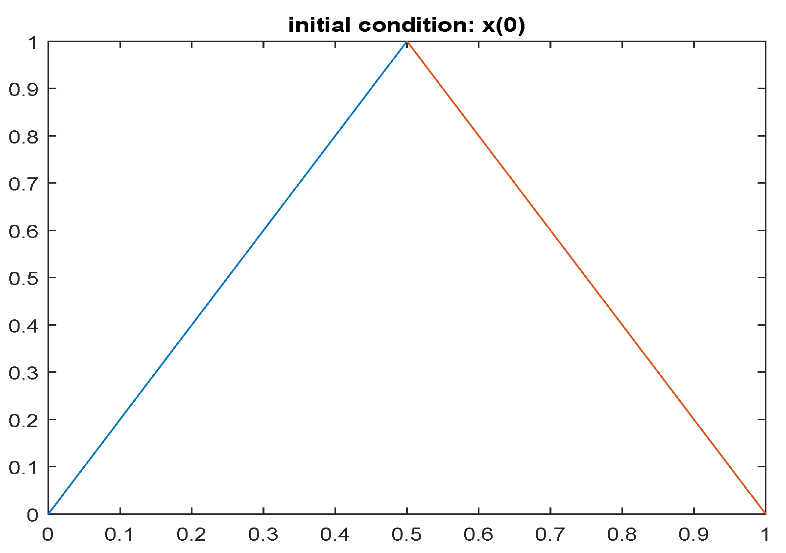
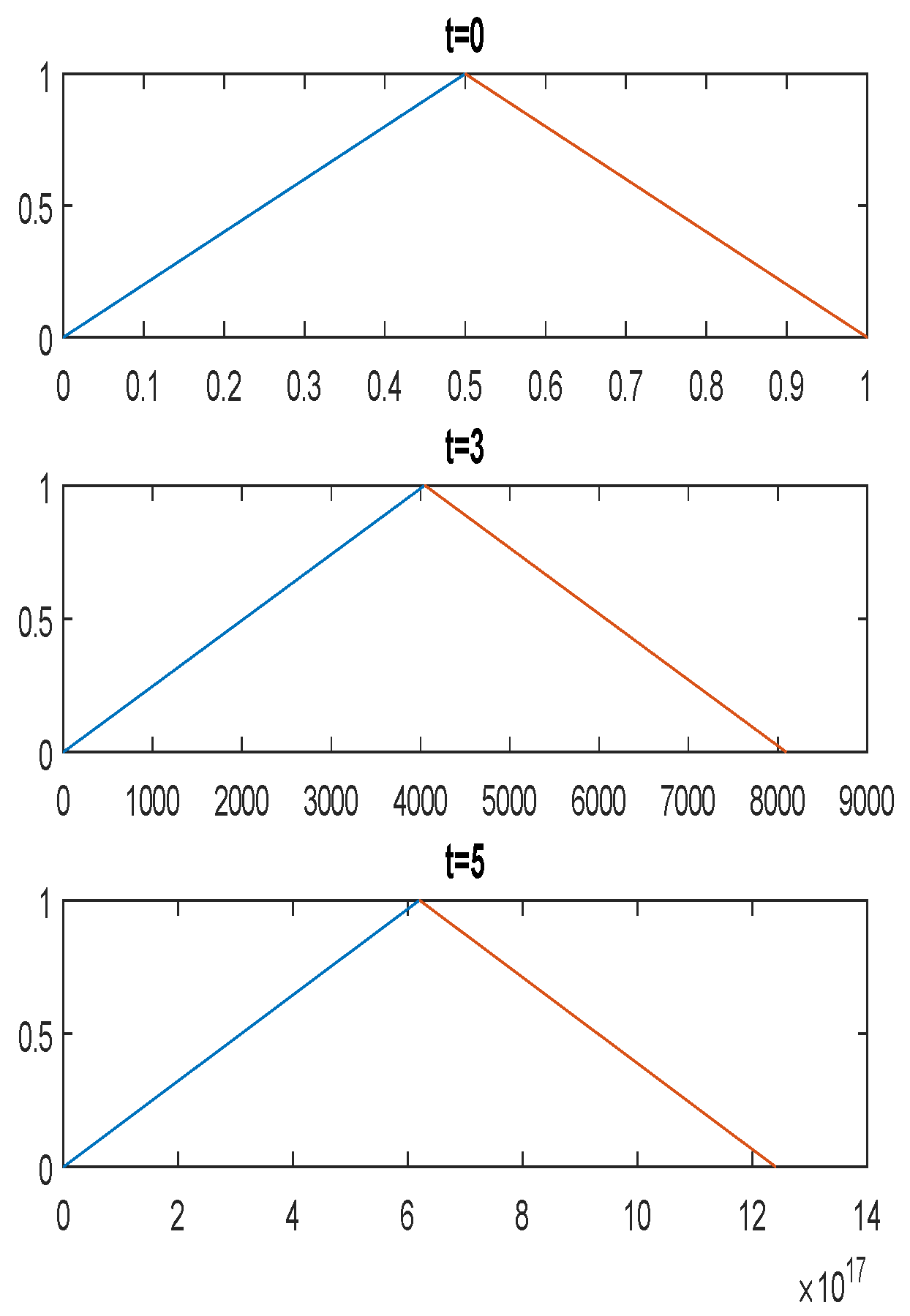
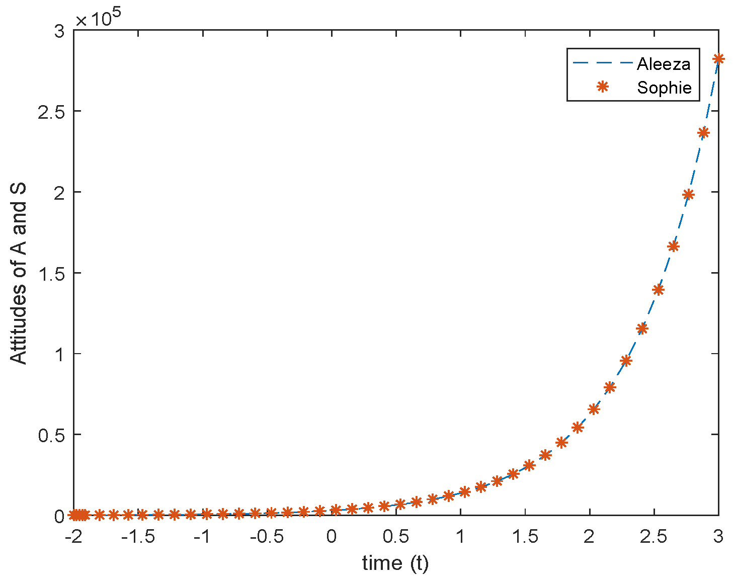
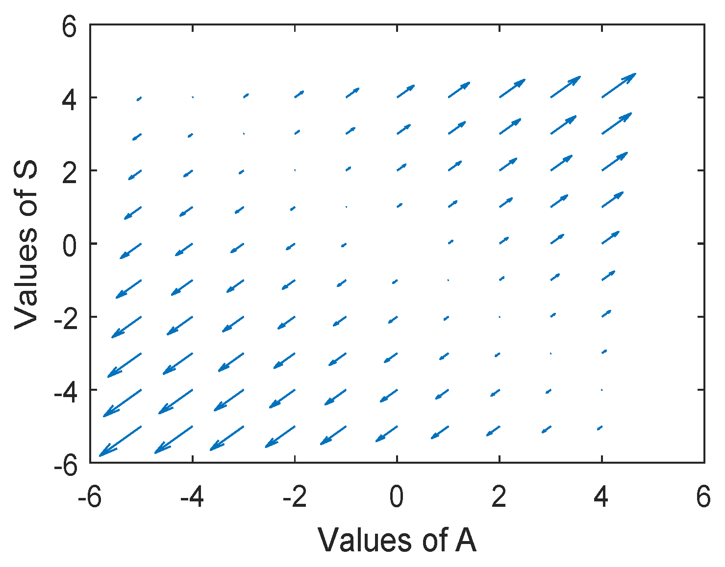
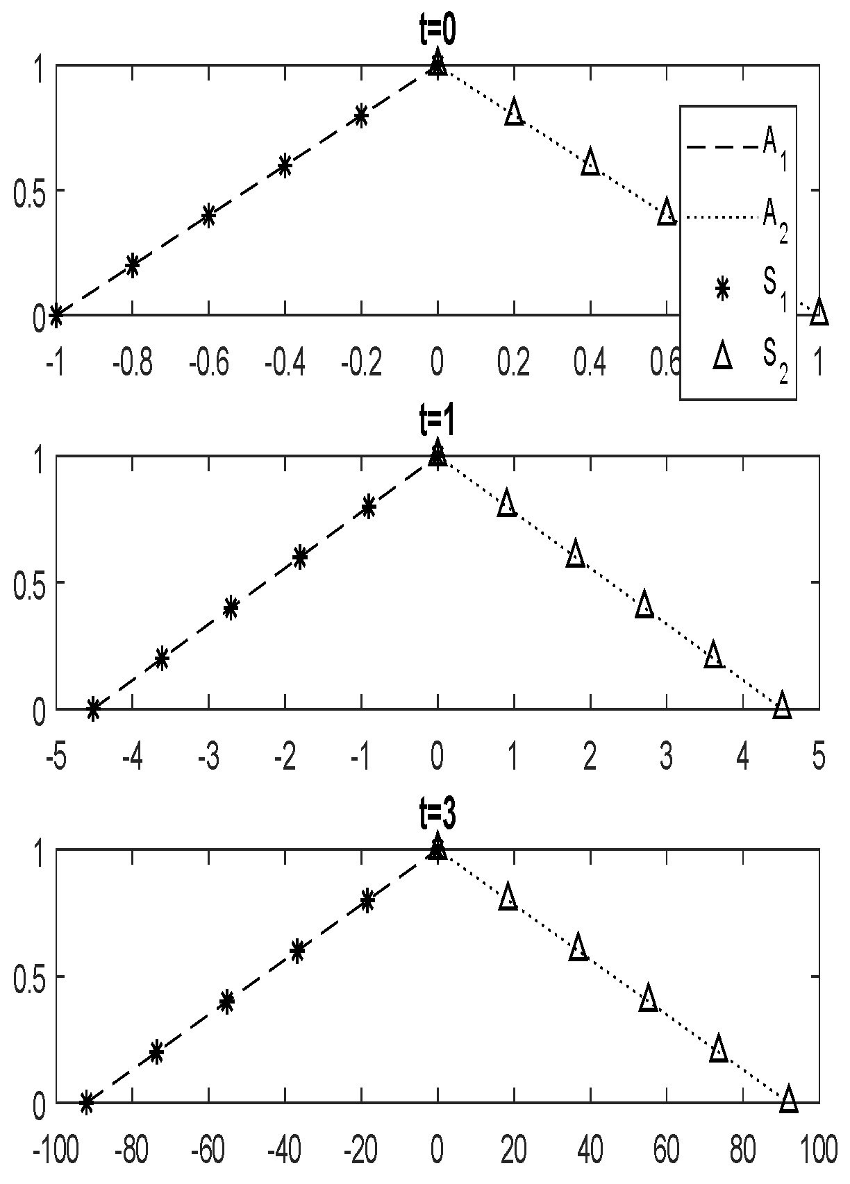
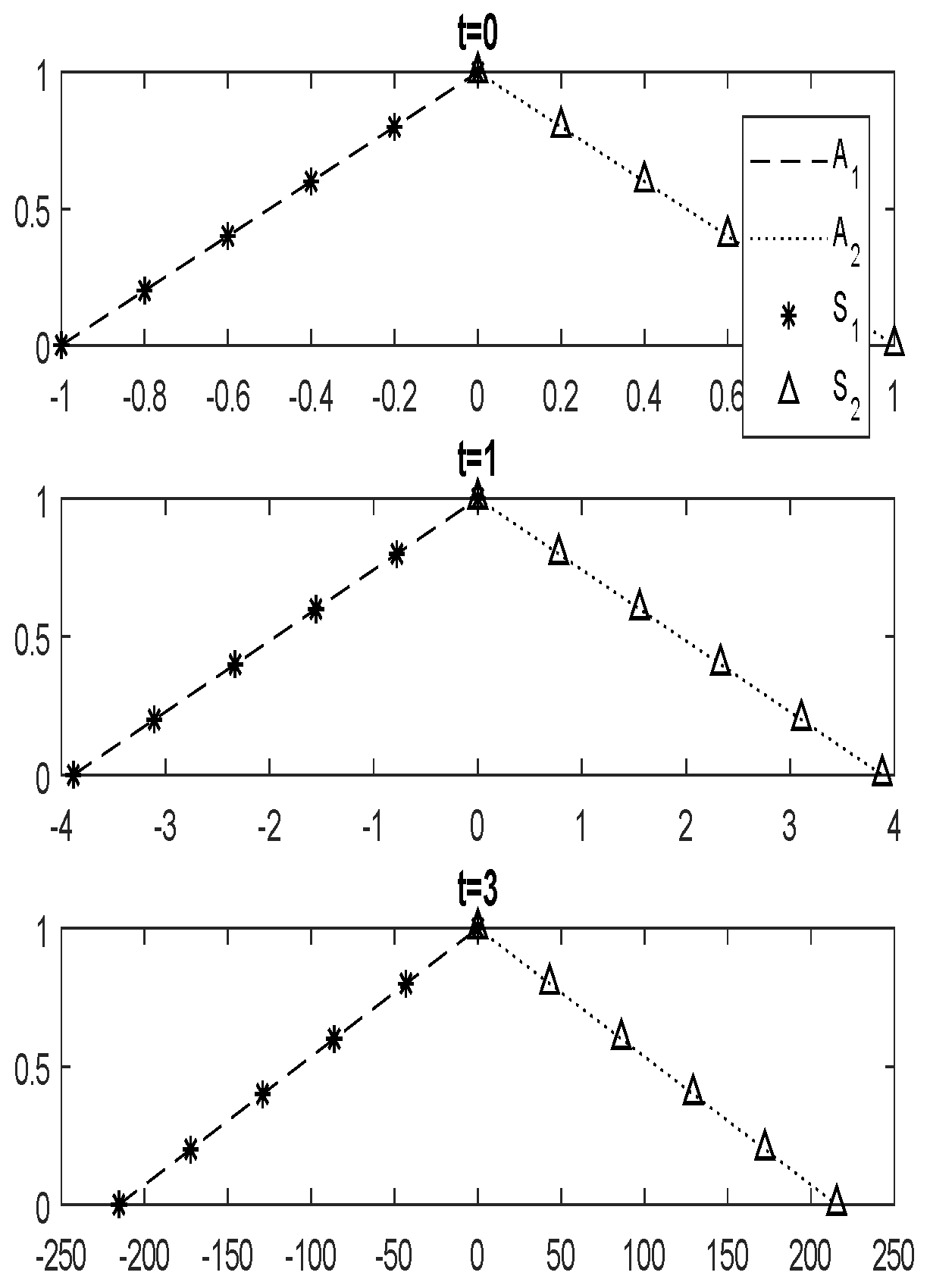
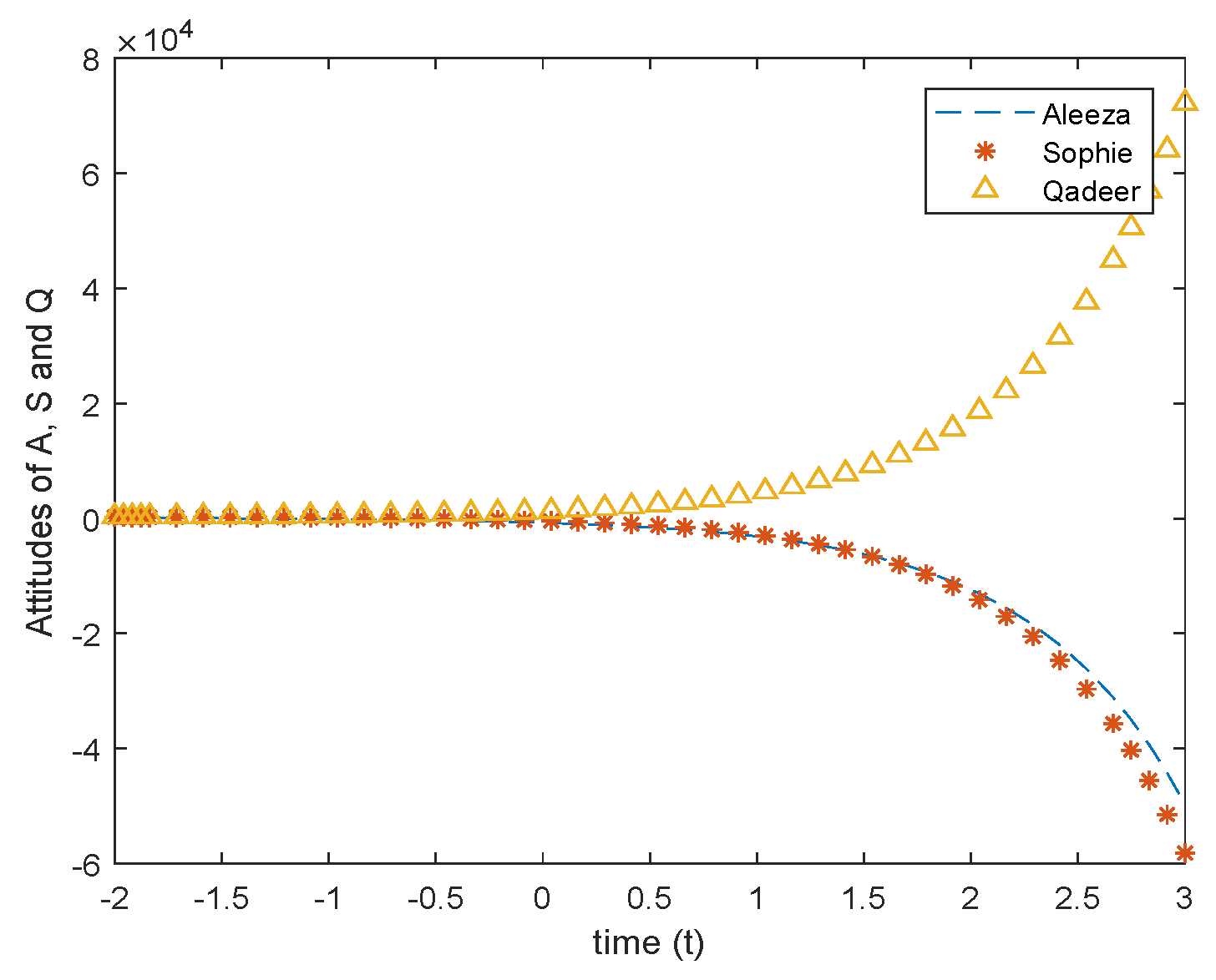
3. An Attitude Analyzer Method Based on Fuzzy Soft Differential Equations

In the process of decision making, the study of a change in attitude of two or three persons after a decision is an interesting area of a research. Indeed, the attitude of two persons when they take same decision may be different to the case when they take the different decisions. This process of investigation contains the following steps:

Step 1: Initial data is taken as DDHFSS under the consideration of m alternatives given by $A_1,A_2,\dots ,A_m$ and n attributes given by $B_1,B_2,\dots ,B_n.$

Step 2: Weight vector $W=\left(w_1,w_2,\dots ,w_n\right)$ with ${\displaystyle \sum _{i=1}^n{w}_i=1}$ is considered for each person. Different weight vectors are considered for different persons.

Step 3: TOPSIS is used as described by Eraslan and Karaaslan [16] to obtain the co-efficients of relative closeness $RC\left(A_j\right)=c_j$ where the distance measure given in Definition 6 is used with $\lambda =1$ to calculate the distances of the values from positive and negative ideal solutions.

Step 4: Optimal fuzzy soft constants $a_{P_j}^i$$(i,j=1,2)$ are chosen from $RC\left(A_j\right)=c_j,$$j=1,2,\dots ,m$ while constructing a dynamical system (2). If two persons select same alternative, then we have

$$a_{P_j}^i=\left\{\begin{array}{c}max\left(c_j\right)if\hfill \\ max\left(max\left(c_j\right),max\left(1-c_j\right)\right)=max\left(c_j\right)\hfill \\ -max\left(1-c_j\right)if\hfill \\ max\left(max\left(c_j\right),max\left(1-c_j\right)\right)=max\left(1-c_j\right)\hfill \end{array}\right.$$

If two persons select different alternatives, then we have

$$a_{P_j}^i=\left\{\begin{array}{cc}max\left(c_j\right)\hfill & ifi=j\hfill \\ -max\left(1-c_j\right)\hfill & ifi\ne j\hfill \end{array}\right.$$

In the case of a third person interference, the following system is considered which is an extension of the system (2) and inspiration of the model presented by Sprott [30].

$$\begin{array}{c}\frac{d{P}_1}{dt}=a_{P_1}^1{P}_1+a_{P_2}^1{P}_2+a_{P_3}^1{P}_3\\ \frac{d{P}_2}{dt}=a_{P_1}^2{P}_1+a_{P_2}^2{P}_2+a_{P_3}^2{P}_3\\ \frac{d{P}_3}{dt}=a_{P_1}^3{P}_1+a_{P_2}^3{P}_2+a_{P_3}^3{P}_3\end{array}$$

(3)

where $a_{P_i}^i$ and $a_{P_j}^i$ denote the effect on $ith$ person of their internal feelings and $jth$ person’s feelings, respectively, and each $\frac{d{P}_i}{dt}$ represent the future attitude of three persons over a time. Note that the state-space is 9 dimensional in this case. Each person has feelings of two types (positive and negative) and hence there are 18 parameters if each person adopts different attitudes towards the others. Some out of the several cases are as under:

(1)

if $a_{P_1}^1>0$, $a_{P_2}^1>0$, $a_{P_3}^1<0$ ($P_1,$$P_2$ both agree for particular decision, but $P_3$ do not agree).

(2)

if $a_{P_1}^1<0$, $a_{P_2}^1<0$, $a_{P_3}^1>0$ ($P_1,$$P_2$ disagree with $P_3$, but $P_3$ encourage them for a particular decision).

(3)

$a_{P2}^1=0$ ($P_2$ has no feeling for $P_1$).

Step 5: Future attitude of two or three persons is observed through the line graphs and phase portraits. A phase portrait is a graphical tool to visualize how the solutions of a given system of differential equations would behave in the long run.

The following example shows the attitude of two persons after a decision and effect of the third person’s interference on their attitudes.

Example 1.

Aleeza and Sophie want to get admission into a senior school. They have five different choices $A_1$, $A_2$, $A_3$, $A_4$ and $A_5$ for the school. They will make the decision under the consideration of four attributes, $B_1$: monthly fee, $B_2$: distance from the residence, $B_3$: reputation and $B_4$: curriculum. They will consider the weight vectors $\left[\begin{array}{cccc}0.2& 0.3& 0.2& 0.3\end{array}\right]$ and $\left[\begin{array}{cccc}0.1& 0.2& 0.3& 0.4\end{array}\right]$, respectively, for the attributes. Analysis of their future attitude is based on the following steps.

Step 1: A dual hesitant fuzzy soft set representing expert opinion is constructed, which is given by

Table 1. Decision set.

	${\mathit{B}}_1$	${\mathit{B}}_2$	${\mathit{B}}_3$	${\mathit{B}}_4$
$A_1$	$\left(\left\{0.6\right\},\left\{0.2\right\}\right)$	$\left(\left\{0.5\right\},\left\{0.4\right\}\right)$	$\left(\left\{0.1,0.4\right\},\left\{0.3,0.4\right\}\right)$	$\left(\left\{0.5,0.6\right\},\left\{0.2,0.3\right\}\right)$
$A_2$	$\left(\left\{0.5\right\},\left\{0.3\right\}\right)$	$\left(\left\{0.7\right\},\left\{0.2\right\}\right)$	$\left(\left\{0.2,0.3,0.5\right\},\left\{0.3,0.5\right\}\right)$	$\left(\left\{0.4,0.5,0.6\right\},\left\{0.1,0.2\right\}\right)$
$A_3$	$\left(\left\{0.4\right\},\left\{0.4\right\}\right)$	$\left(\left\{0.8\right\},\left\{0.1\right\}\right)$	$\left(\left\{0.6,0.7\right\},\left\{0.2,0.3\right\}\right)$	$\left(\left\{0.5,0.6\right\},\left\{0.3,0.4\right\}\right)$
$A_4$	$\left(\left\{0.5,\right\},\left\{0.3\right\}\right)$	$\left(\left\{0.6\right\},\left\{0.3\right\}\right)$	$\left(\left\{0.5,0.6,0.9\right\},\left\{0.1\right\}\right)$	$\left(\left\{0.8,0.9\right\},\left\{0.1\right\}\right)$
$A_5$	$\left(\left\{0.6\right\},\left\{0.3\right\}\right)$	$\left(\left\{0.5\right\},\left\{0.4\right\}\right)$	$\left(\left\{0.3,0.5\right\},\left\{0.3,0.4\right\}\right)$	$\left(\left\{0.7,0.8\right\},\left\{0.1,0.2\right\}\right)$

.

Step 2: Weighted decision sets for $\left[\begin{array}{cccc}0.2& 0.3& 0.2& 0.3\end{array}\right]$ and $\left[\begin{array}{cccc}0.1& 0.2& 0.3& 0.4\end{array}\right]$ are formed, which are shown in

Table 2. Weighted decision set for Aleeza.

	${\mathit{B}}_1$	${\mathit{B}}_2$	${\mathit{B}}_3$	${\mathit{B}}_4$
$A_1$	$\left(\left\{0.1674\right\},\left\{0.7247\right\}\right)$	$\left(\left\{0.1877\right\},\left\{0.7596\right\}\right)$	$\left(\left\{0.0208,0.0971\right\},\left\{0.7860,0.9028\right\}\right)$	$\left(\left\{0.1877,0.2403\right\},\left\{0.6170,0.6968\right\}\right)$
$A_2$	$\left(\left\{0.1294\right\},\left\{0.7860\right\}\right)$	$\left(\left\{0.3031\right\},\left\{0.6170\right\}\right)$	$\left(\left\{0.0436,0.0688,0.1294\right\},\left\{0.7860,0.8705\right\}\right)$	$\left(\left\{0.1420,0.1877,0.2403\right\},\left\{0.5011,0.6170\right\}\right)$
$A_3$	$\left(\left\{0.0971\right\},\left\{0.9028\right\}\right)$	$\left(\left\{0.3829\right\},\left\{0.5011\right\}\right)$	$\left(\left\{0.1674,0.2139\right\},\left\{0.7247,0.7860\right\}\right)$	$\left(\left\{0.1877,0.2403\right\},\left\{0.6968,0.7596\right\}\right)$
$A_4$	$\left(\left\{0.1294\right\},\left\{0.7860\right\}\right)$	$\left(\left\{0.2403\right\},\left\{0.6968\right\}\right)$	$\left(\left\{0.1294,0.1674,0.3690\right\},\left\{0.6309\right\}\right)$	$\left(\left\{0.3829,0.4988\right\},\left\{0.5011\right\}\right)$
$A_5$	$\left(\left\{0.1674\right\},\left\{0.7860\right\}\right)$	$\left(\left\{0.1877\right\},\left\{0.7596\right\}\right)$	$\left(\left\{0.0688,0.1294\right\},\left\{0.7860,0.9028\right\}\right)$	$\left(\left\{0.3031,0.3829\right\},\left\{0.5011,0.6170\right\}\right)$

and

Table 3. Weighted decision set for Sophie.

	${\mathit{B}}_1$	${\mathit{B}}_2$	${\mathit{B}}_3$	${\mathit{B}}_4$
$A_1$	$\left(\left\{0.0875\right\},\left\{0.8513\right\}\right)$	$\left(\left\{0.1294\right\},\left\{0.8325\right\}\right)$	$\left(\left\{0.0311,0.1420\right\},\left\{0.6968,0.7596\right\}\right)$	$\left(\left\{0.2421,0.3068\right\},\left\{0.5253,0.6178\right\}\right)$
$A_2$	$\left(\left\{0.0669\right\},\left\{0.8865\right\}\right)$	$\left(\left\{0.2139\right\},\left\{0.7247\right\}\right)$	$\left(\left\{0.0647,0.1014,0.1877\right\},\left\{0.6968,0.8122\right\}\right)$	$\left(\left\{0.1848,0.2421,0.3068\right\},\left\{0.3981,0.5253\right\}\right)$
$A_3$	$\left(\left\{0.0497\right\},\left\{0.9124\right\}\right)$	$\left(\left\{0.2752\right\},\left\{0.6309\right\}\right)$	$\left(\left\{0.2403,0.3031\right\},\left\{0.6170,0.6968\right\}\right)$	$\left(\left\{0.2421,0.3068\right\},\left\{0.6178,0.6931\right\}\right)$
$A_4$	$\left(\left\{0.0669\right\},\left\{0.8865\right\}\right)$	$\left(\left\{0.1674\right\},\left\{0.7860\right\}\right)$	$\left(\left\{0.1877,0.2403,0.4988\right\},\left\{0.5011\right\}\right)$	$\left(\left\{0.4746,0.6018\right\},\left\{0.3981\right\}\right)$
$A_5$	$\left(\left\{0.0875\right\},\left\{0.8865\right\}\right)$	$\left(\left\{0.1294\right\},\left\{0.8325\right\}\right)$	$\left(\left\{0.1014,0.1877\right\},\left\{0.6968,0.7596\right\}\right)$	$\left(\left\{0.3821,0.4746\right\},\left\{0.3981,0.5253\right\}\right)$

, respectively.

Step 3: Positive ideal solutions and negative ideal solutions from Table 2 and Table 3 are represented in

Table 4. Positive and negative ideal solutions for Aleeza.

	${\mathit{B}}_1$	${\mathit{B}}_2$	${\mathit{B}}_3$	${\mathit{B}}_4$
$A^{+}$	$\left(0.0971,0.9028\right)$	$\left(0.1877,0.7596\right)$	$\left(0.2139,0.6309\right)$	$\left(0.4988,0.5011\right)$
$A^{-}$	$\left(0.1674,0.7247\right)$	$\left(0.3829,0.5011\right)$	$\left(0.0208,0.9028\right)$	$\left(0.1420,0.7596\right)$

and

Table 5. Positive and negative ideal solutions for Sophie.

	${\mathit{B}}_1$	${\mathit{B}}_2$	${\mathit{B}}_3$	${\mathit{B}}_4$
$A_1$	$\left(0.0497,0.9124\right)$	$\left(0.1294,0.8325\right)$	$\left(0.4988,0.5011\right)$	$\left(0.6018,0.3981\right)$
$A_2$	$\left(0.0875,0.8513\right)$	$\left(0.2752,0.6309\right)$	$\left(0.0311,0.8122\right)$	$\left(0.1848,0.6931\right)$

, respectively.

The following are the distances $d(A_i,A^{+})$ and $d(A_i,A^{-})$ calculated from Tablse Table 2 and Table 4 using Definition 6.

$$\begin{array}{c}d(A_1,A^{+})=0.1321\\ d(A_2,A^{+})=0.1426\\ d(A_3,A^{+})=0.1391\\ d(A_4,A^{+})=0.0604\\ d(A_5,A^{+})=0.0910\end{array}$$

$$\begin{array}{c}d(A_1,A^{-})=0.0906\\ d(A_2,A^{-})=0.0804\\ d(A_3,A^{-})=0.1143\\ d(A_4,A^{-})=0.1807\\ d(A_5,A^{-})=0.1315\end{array}.$$

Co-efficients of relative closeness are given as:

$RC\left(A_1\right)=0.4068,$$RC\left(A_2\right)=0.3605,$$RC\left(A_3\right)=0.4510,$$RC\left(A_4\right)=0.7494,$$RC\left(A_5\right)=0.5910$.

We now rank the four alternatives for Aleeza as follows:

$$A_2<A_1<A_3<A_5<A_4.$$

Now, the distances $d(A_i,A^{+})$ and $d(A_i,A^{-})$ are calculated from Table 3 and Table 5:

$$\begin{array}{c}d(A_1,A^{+})=0.1549\\ d(A_2,A^{+})=0.1718\\ d(A_3,A^{+})=0.1643\\ d(A_4,A^{+})=0.0621\\ d(A_5,A^{+})=0.1276\end{array}$$

$$\begin{array}{c}d(A_1,A^{-})=0.1418\\ d(A_2,A^{-})=0.0772\\ d(A_3,A^{-})=0.1\\ d(A_4,A^{-})=0.1947\\ d(A_5,A^{-})=0.1318.\end{array}$$

Note that $RC\left(A_1\right)=0.4779,$$RC\left(A_2\right)=0.3100,$$RC\left(A_3\right)=0.3783,$$RC\left(A_4\right)=0.7581,$$RC\left(A_5\right)=0.5080$. Ranking the four alternatives, we have

$$A_2<A_3<A_1<A_5<A_4.$$

Step 4: A system of fuzzy soft differential equations constructed as (2) using the co-efficients of relative closeness is given by

$$\begin{array}{c}\frac{dA}{dt}=aA+bS\\ \frac{dS}{dt}=cA+dS,\end{array}$$

where A and S are the variables used for Aleeza and Sophie, respectively. Since they choose the same alternative $A_4$, so we take $a=c=0.7494$ and $b=d=0.7581$

$$\begin{array}{c}\frac{dA}{dt}=0.7494A+0.7581S\\ \frac{dS}{dt}=0.7494A+0.7581S\end{array}$$

(4)

Line graphs for Aleeza and Sophie in Figure 3 overlap, which is an indication of the same behaviour in the future, and Figure 4 shows that the system is unstable.

The same result is obtained when the following fuzzy initial conditions (FICs) are applied (Figure 5).

$$\begin{array}{ccc}{P}_1\left(0\right)=(-1+r,1-r)& & r\in [0,1]\\ P_2\left(0\right)=(-1+r,1-r)& & r\in [0,1]\end{array}$$

Then

$$\begin{array}{ccc}{P}_1=((-1+r)e^{1.5075t},(1-r)e^{1.5075t}),& & r\in [0,1]\\ P_2=((-1+r)e^{1.5075t},(1-r)e^{1.5075t}),& & r\in [0,1]\end{array}$$

$A_1$ and $S_1$ represent the increasing parts of the solution and can also be denoted as $\underset{\sim }{A}$ and $\underset{\sim }{S}$, respectively. $A_2$ and $S_2$ represent the decreasing part of the solution and can also be denoted as $\stackrel{\sim }{A}$ and $\stackrel{\sim }{S}$, respectively.

If there is a third person named “Qadeer” who talks with Aleeza and Sophie about their decisions and informs them about the same kind of decision that he had taken one year back. Then, the changes in their future attitudes are also proportional to Qadeer’s decision.

Case 1: Suppose that Qadeer had the values of relative closeness given by:

$RC\left(A_1\right)=0.4468,$$RC\left(A_2\right)=0.3570,$$RC\left(A_3\right)=0.5620,$$RC\left(A_4\right)=0.6020,$$RC\left(A_5\right)=0.6224$.

Since Aleeza and Sophie do not agree with Qadeer’s decision and Qadeer does not satisfy Aleeza and Sophie, so the coefficients $a_Q^A=$$a_Q^S=-\left(1-0.3570\right)=-0.643$, $a_Q^Q=0.6224$, $a_A^Q=-\left(1-0.3605\right)=-0.6495$, $a_S^Q=-\left(1-0.31\right)=-0.69$ will be used in system (4), which are obtained from (3) by replacing $P_1,P_2$ and $P_3$ with $A,S$ and Q, respectively. Thus,

$$\begin{array}{c}\frac{dA}{dt}=a_A^{A}A+a_S^{A}S+a_Q^{A}Q\\ \frac{dS}{dt}=a_A^{S}A+a_S^{S}S+a_Q^{S}Q\\ \frac{dQ}{dt}=a_A^{Q}A+a_S^{Q}S+a_Q^{Q}Q\end{array}$$

(5)

$$\begin{array}{c}\frac{dA}{dt}=0.7494A+0.7581S-0.643Q\\ \frac{dS}{dt}=0.7494A+0.7581S-0.643Q\\ \frac{dQ}{dt}=-0.6495A-0.69S+0.6224Q\end{array}$$

(6)

Line graph in Figure 6 ($A_1$ and $S_1$ stand for increasing parts of triangular fuzzy numbers, $A_2$ and $S_2$ stand for decreasing parts of triangular fuzzy numbers) shows that Aleeza and Sophie will show the same behaviour in the future. It means that there is no change due to interference of Qadeer. Furthermore, the graphs for Aleeza and Sophie are overlapping. Figure 7 is a projection of $3D$$(A,S,Q)$ on $AS$ plane and shows that the system is unstable.

Case 2: Suppose Aleeza and Sophie have the following $RC\left(A_i\right),$ for $i=1,2,3,4,5$, respectively:

$RC\left(A_1\right)=0.4007,$$RC\left(A_2\right)=0.5204,$$RC\left(A_3\right)=0.5431,$$RC\left(A_4\right)=0.4620,$$RC\left(A_5\right)=0.4413$

$RC\left(A_1\right)=0.6270,$$RC\left(A_2\right)=0.5947,$$RC\left(A_3\right)=0.6542,$$RC\left(A_4\right)=0.7214,$$RC\left(A_5\right)=0.6621$ and they choose different schools/alternatives for them.

Suppose a third person, Qadeer, had the following relative closeness coefficients for five alternatives:

$RC\left(A_1\right)=0.4207,$$RC\left(A_2\right)=0.4973,$$RC\left(A_3\right)=0.5276,$$RC\left(A_4\right)=0.6234,$$RC\left(A_5\right)=0.6750$

In this case, the following coefficients are used in system (5)

$$\begin{array}{c}{a}_A^A=0.5431\\ a_S^A=a_S^Q=-(1-0.5947)=-0.4053\\ a_Q^A=a_Q^S=-(1-0.4207)=-0.5793\\ a_A^S=a_A^Q=-(1-0.4007)=-0.5993\\ a_S^S=0.7214\\ a_Q^Q=0.6750\end{array}$$

and system (7) is obtained to check the future attitude of three persons

$$\begin{array}{c}\frac{dA}{dt}=0.5431A-0.4053S-0.5793Q\\ \frac{dS}{dt}=-0.5993A+0.7214S-0.5793Q\\ \frac{dQ}{dt}=-0.5993A-0.4053S+0.675Q\end{array}$$

(7)

Line graph in Figure 8 shows that Aleeza and Sophie will show different behaviours in the future, and Figure 9 shows that the system is stable.

Case 3: If we assume that Aleeza and Sophie have no effect on each other, i.e., $a_S^A=a_A^S=0$, then the system (7) reduces to the following system (8):

$$\begin{array}{c}\frac{dA}{dt}=-0.5893Q+0.5431A\\ \frac{dS}{dt}=-0.5893Q+0.7214S\\ \frac{dQ}{dt}=0.6750Q-0.5993A-0.4053S\end{array}$$

(8)

The line graph in Figure 10 shows that Aleeza and Sophie will exhibit almost the same behaviour in the future, but Qadeer will behave differently. Note that Figure 11 indicates that the system is of saddle type. This result can also be obtained by using FICs.

4. Conclusions

The system of linear differential equations is advantageous for the analysis of experts’ attitudes and FICs are appropriate due to the association with uncertainties. The line graph represents whether the experts agree with each other or not in the future, whereas phase portrait is essential to check the stability of the system. Interference of a third person in a decision taken by two persons affects their future attitudes. They may rethink their decisions positively or negatively. If two persons make the same decision, they also agree with each other in the future unless a third person interferes between them with a different opinion. This kind of result may also be examined by using some MCDM method other than TOPSIS. This research work is inspired by Sprott [30] and would also contribute to the post-consensus analysis, group decision processes, interpersonal influences and opinion dynamics due to some research gaps referred to the interferences.

References

1. Torra, V.; Narukawa, Y. On Hesitant Fuzzy Sets and Decision. In Proceedings of the 2009 IEEE International Conference on Fuzzy Systems, Jeju, Korea, 20–24 August 2009. [Google Scholar]
2. Torra, V. Hesitant fuzzy sets. Int. J. Intell. Syst. 2010, 25, 529–539. [Google Scholar] [CrossRef]
3. Wang, B.; Liang, J.; Pang, J. Deviation degree: A perspective on score functions in hesitant fuzzy sets. Int. J. Fuzzy Syst. 2019, 21, 2299–2317. [Google Scholar] [CrossRef]
4. Farhadinia, B. Information measures for hesitant fuzzy sets and interval-valued hesitant fuzzy sets. Inf. Sci. 2013, 240, 129–144. [Google Scholar] [CrossRef]
5. Wang, F.; Li, X.; Chen, X. Hesitant fuzzy soft set and its applications in multicriteria decision making. J. Appl. Math. 2014, 2014, 643785. [Google Scholar] [CrossRef]
6. Peng, X.; Yang, Y. Interval-valued hesitant fuzzy soft sets and their application in Decision Making. Fundam. Inform. 2015, 141, 71–93. [Google Scholar] [CrossRef]
7. Atanassov, K.T. Intutionistic fuzzy sets. Fuzzy Sets Syst. 1986, 20, 87–96. [Google Scholar] [CrossRef]
8. Grzegorzewski, P. Distances between intuitionistic fuzzy sets and/or interval-valued fuzzy sets based on the Hausdorff metric. Fuzzy Sets syst. 2004, 148, 319–328. [Google Scholar] [CrossRef]
9. Zhu, B.; Xu, Z.; Xia, M. Dual hesitant fuzzy sets. J. Appl. Math. 2012, 2012, 879629. [Google Scholar] [CrossRef]
10. Singh, P. Distance and similarity measures for multiple attribute decision making with dual hesitant fuzzy sets. Comput. Appl. Math. 2017, 36, 111–126. [Google Scholar] [CrossRef]
11. Zhang, H.; Shu, L. Dual hesitant fuzzy soft set and its properties. In Fuzzy Systems & Operations Research and Management; Cao, B.Y., Liu, Z.L., Zhong, Y.B., Mi, H.H., Eds.; Springer International Publishing: Cham, Switzerland, 2016; pp. 171–182. [Google Scholar]
12. Garg, H.; Arora, R. Distance and similarity measures for dual hesitant fuzzy soft sets and their applications in multicriteria decision making problem. Int. J. Uncertain. Quantif. 2017, 7, 229–248. [Google Scholar] [CrossRef]
13. Aruldoss, M.; Lakshmi, T.M.; Venkatesan, V.P. A survey on multicriteria decision making methods and its applications. Am. J. Inf. Syst. 2013, 1, 31–43. [Google Scholar]
14. Beg, I.; Rashid, T. Hesitant 2-tuple linguistic information in multiple attributes group decision making. J. Intell. Fuzzy Syst. 2016, 30, 109–116. [Google Scholar] [CrossRef]
15. Eraslan, S.; Cagman, N. A decision making method by combining TOPSIS and grey relation method under fuzzy soft sets. Sigma J. Eng. Nat. Sci. 2017, 8, 53–64. [Google Scholar]
16. Eraslan, S.; Karaaslan, F. A group decision making method based on TOPSIS under fuzzy soft environment. J. New Theory 2015, 3, 30–40. [Google Scholar]
17. Joshi, D.; Kumar, S. Intuitionistic fuzzy entropy and distance measure based TOPSIS method for multi-criteria decision making. Egypt. Inform. J. 2004, 15, 97–104. [Google Scholar] [CrossRef]
18. Rani, P.; Mishra, A.R.; Rezaei, G.; Liao, H.; Mardani, A. Extended pythagorean fuzzy TOPSIS method based on similarity measure for sustainable recycling partner selection. Int. J. Fuzzy Syst. 2020, 22, 735–747. [Google Scholar] [CrossRef]
19. Wang, L.; Wang, Q.; Xu, S.; Ni, M. Distance and similarity measures of dual hesitant fuzzy sets with their applications to multiple attribute decision making. In Proceedings of the 2014 IEEE International Conference on Progress in Informatics and Computing, Shanghai, China, 16–18 May 2014. [Google Scholar]
20. Perez-Benitez, V.; Gemar, G.; Hernandez, M. Multi-criteria analysis for business location decisions. Mathematics 2021, 9, 2615. [Google Scholar] [CrossRef]
21. Selvaraj, J.; Majumdar, A. A new ranking method for interval-valued intuitionistic fuzzy numbers and its application in Multi-criteria decision-making. Mathematics 2021, 9, 2647. [Google Scholar] [CrossRef]
22. Zadeh, L.A. Toward a generalized theory of uncertainty (GTU) an outline. Inf. Sci. 2005, 172, 140. [Google Scholar] [CrossRef]
23. Puri, M.L.; Ralescu, D.A. Differentials of fuzzy functions. J. Math. Anal. 1983, 91, 552–558. [Google Scholar] [CrossRef] [Green Version]
24. Kaleva, O. Fuzzy differential equations. Fuzzy Sets Syst. 1987, 24, 301–317. [Google Scholar] [CrossRef]
25. Buckley, J.J.; Feuring, T. Fuzzy differential equations. Fuzzy Sets Syst. 2000, 110, 43–54. [Google Scholar] [CrossRef]
26. Mizukoshi, M.T.; Barros, L.C.; Chalco-Cano, Y.; Roman-Flores, H.; Bassanezi, R.C. Fuzzy differential equations and the extension principle. Inf. Sci. 2007, 177, 3627–3635. [Google Scholar] [CrossRef]
27. Effati, S.; Pakdaman, M. Artificial neural network approach for solving fuzzy differential equations. Inf. Sci. 2010, 180, 1434–1457. [Google Scholar] [CrossRef]
28. Beg, I.; Rashid, T.; Jamil, R.N. Human attitude analysis based on fuzzy soft differential equations with bonferroni mean. Comput. Appl. Math. 2018, 37, 2632–2647. [Google Scholar] [CrossRef]
29. Strogatz, S.H. Linear Systems. In Nonlinear Dynamics and Chaos: With Applications to Physics, Biology, Chemistry, and Engineering; Perseus Books Publishing: New York, NY, USA, 1994; pp. 123–144. [Google Scholar]
30. Sprott, J.C. Dynamical models of love. Non-Linear Dyn. Psychol. Life Sci. 2004, 8, 303–313. [Google Scholar]
31. Friedkin, N.; Johnson, E. Social influence network and opinion change. Adv. Group Process. 1999, 16, 1–29. [Google Scholar]
32. Khalid, A.; Beg, I. Influence model of evasive decision makers. J. Intell. Fuzzy Syst. 2019, 37, 2539–2548. [Google Scholar] [CrossRef] [Green Version]
33. Heninger, W.G.; Dennis, A.R.; Hilmer, K.M.N. Individual cognition and Dual-task interference in group support systems. Inf. Syst. Res. 2006, 17, 415–424. [Google Scholar] [CrossRef]
34. Xiao, F. A complex mass function to predict interference effects. IEEE Trans. Cybern. 2021, 1–13. [Google Scholar] [CrossRef]
35. Xu, Z.; Xia, M. Distance and similarity measures for hesitant fuzzy sets. Inf. Sci. 2011, 181, 2128–2138. [Google Scholar] [CrossRef]
36. Kargar, R.; Allahviranloo, T.; Malkhalifeh, M.R.; Jahanshaloo, G.R. A proposed method for solving fuzzy system of linear equations. Sci. World J. 2014, 2014, 782093. [Google Scholar] [CrossRef] [PubMed] [Green Version]
Figure 1. Initial condition.
Mathematics 09 02788 g001
Figure 2. Line graph for the solution.
Mathematics 09 02788 g002
Figure 3. Line graph for differential Equation (4).
Mathematics 09 02788 g003
Figure 4. Phase portrait for differential Equation (4).
Mathematics 09 02788 g004
Figure 5. Line graph for differential Equation (4) with FICs.
Mathematics 09 02788 g005
Figure 6. Line graph for differential Equation (6) with FICs.
Mathematics 09 02788 g006
Figure 7. Phase portrait for differential Equation (6).
Mathematics 09 02788 g007
Figure 8. Line graph for differential Equation (7) with FICs.
Mathematics 09 02788 g008
Figure 9. Phase portrait for differential Equation (7).
Mathematics 09 02788 g009
Figure 10. Line graph for differential Equation (8).
Mathematics 09 02788 g010
Figure 11. Phase portrait for differential Equation (8).
Mathematics 09 02788 g011