Author Contributions
Conceptualization, R.A.R.B., C.C., F.J., M.E., W.A. and A.A.A.; methodology, R.A.R.B., C.C., F.J., M.E., W.A. and A.A.A.; validation, R.A.R.B., C.C., F.J., M.E., W.A. and A.A.A.; writing—review and editing, R.A.R.B., C.C., F.J., M.E., W.A. and A.A.A. All authors have read and agreed to the published version of the manuscript.
Figure 1.
Plots showing different shapes of the pdf of the MKw distribution: (a) decreasing and unimodal shapes and (b) U- and N-shapes.
Figure 1.
Plots showing different shapes of the pdf of the MKw distribution: (a) decreasing and unimodal shapes and (b) U- and N-shapes.
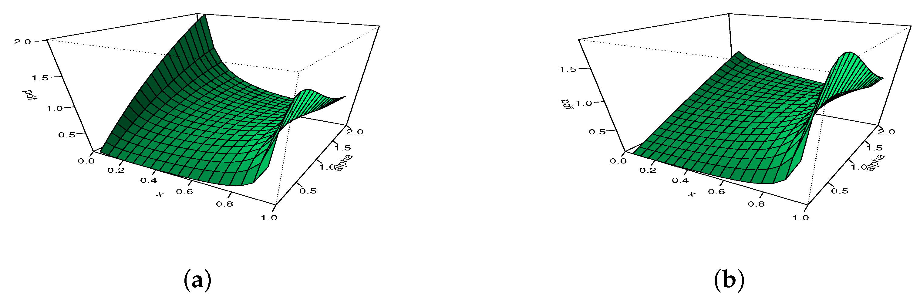
Figure 2.
The 3D plots of the pdf of the MKw distribution for with (a) , (b) , (c) , and (d) .
Figure 2.
The 3D plots of the pdf of the MKw distribution for with (a) , (b) , (c) , and (d) .
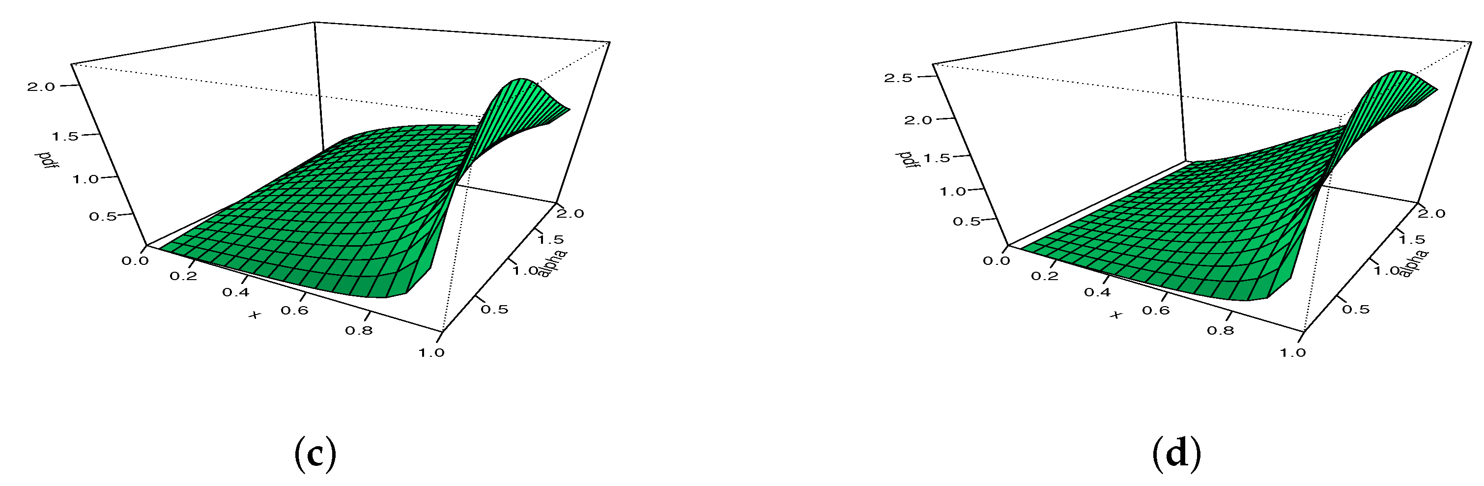
Figure 3.
The 3D plots of the pdf of the MKw distribution for with (a) , (b) , (c) , and (d) .
Figure 3.
The 3D plots of the pdf of the MKw distribution for with (a) , (b) , (c) , and (d) .
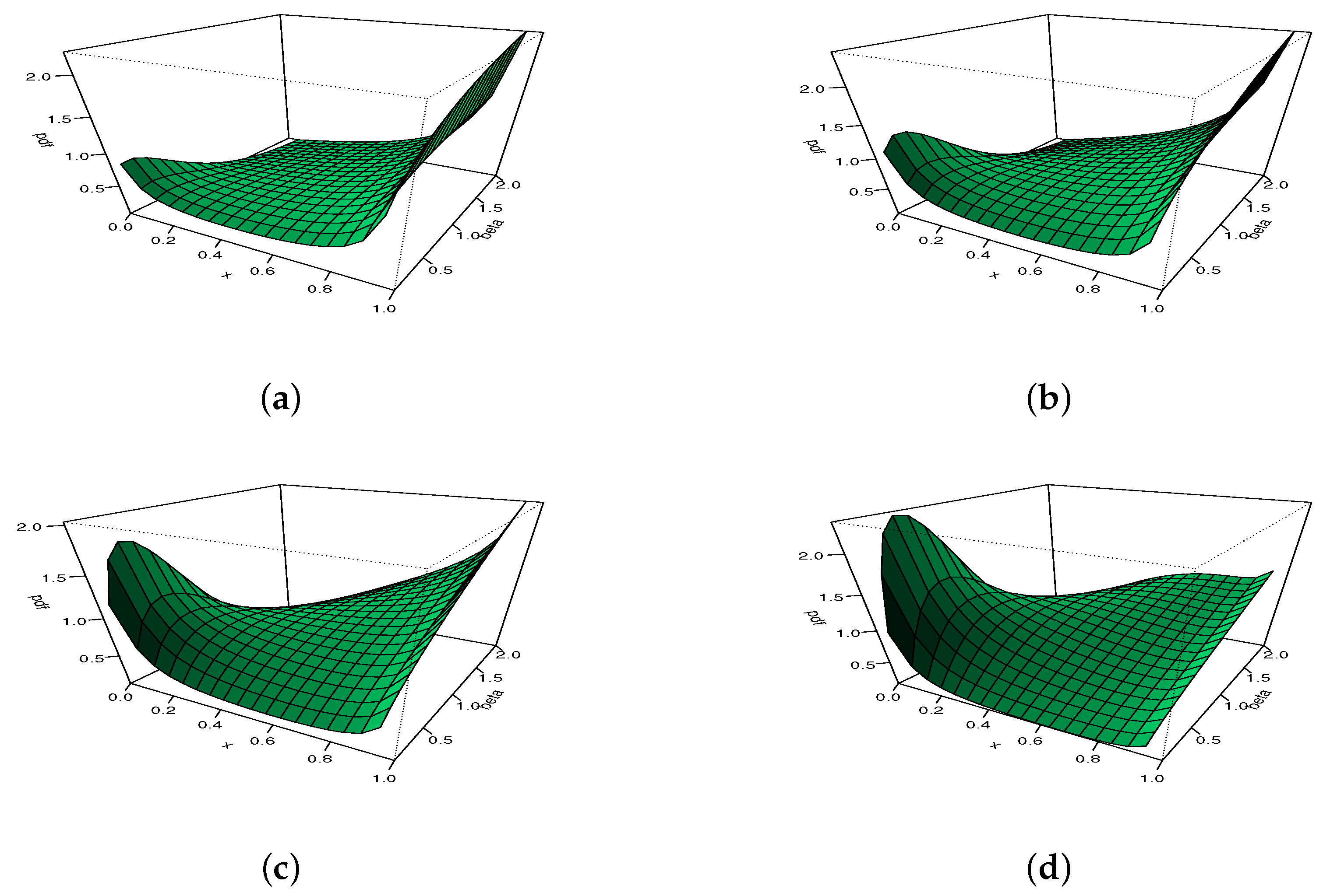
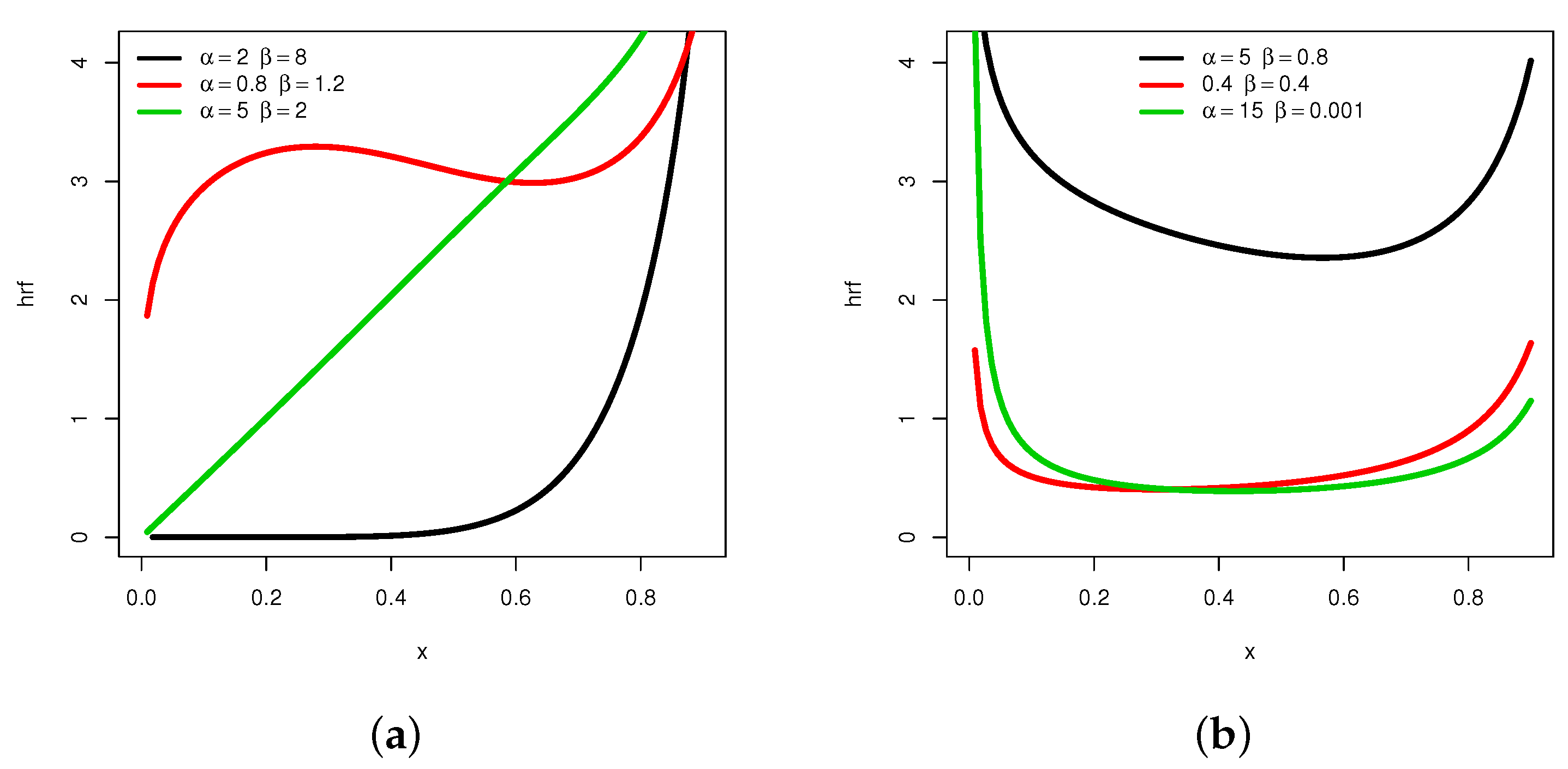
Figure 4.
Plots showing different shapes of the hrf of the MKw distribution: (a) increasing, convex, constant and N-shapes, and (b) U-shapes.
Figure 4.
Plots showing different shapes of the hrf of the MKw distribution: (a) increasing, convex, constant and N-shapes, and (b) U-shapes.
Figure 5.
The 3D plots of the hrf of the MKw distribution for with (a) , (b) , (c) , and (d) .
Figure 5.
The 3D plots of the hrf of the MKw distribution for with (a) , (b) , (c) , and (d) .
Figure 6.
The 3D plots of the hrf of the MKw distribution for with (a) , (b) , (c) , and (d) .
Figure 6.
The 3D plots of the hrf of the MKw distribution for with (a) , (b) , (c) , and (d) .
Figure 7.
The 3D plots of QS and QK for .
Figure 7.
The 3D plots of QS and QK for .
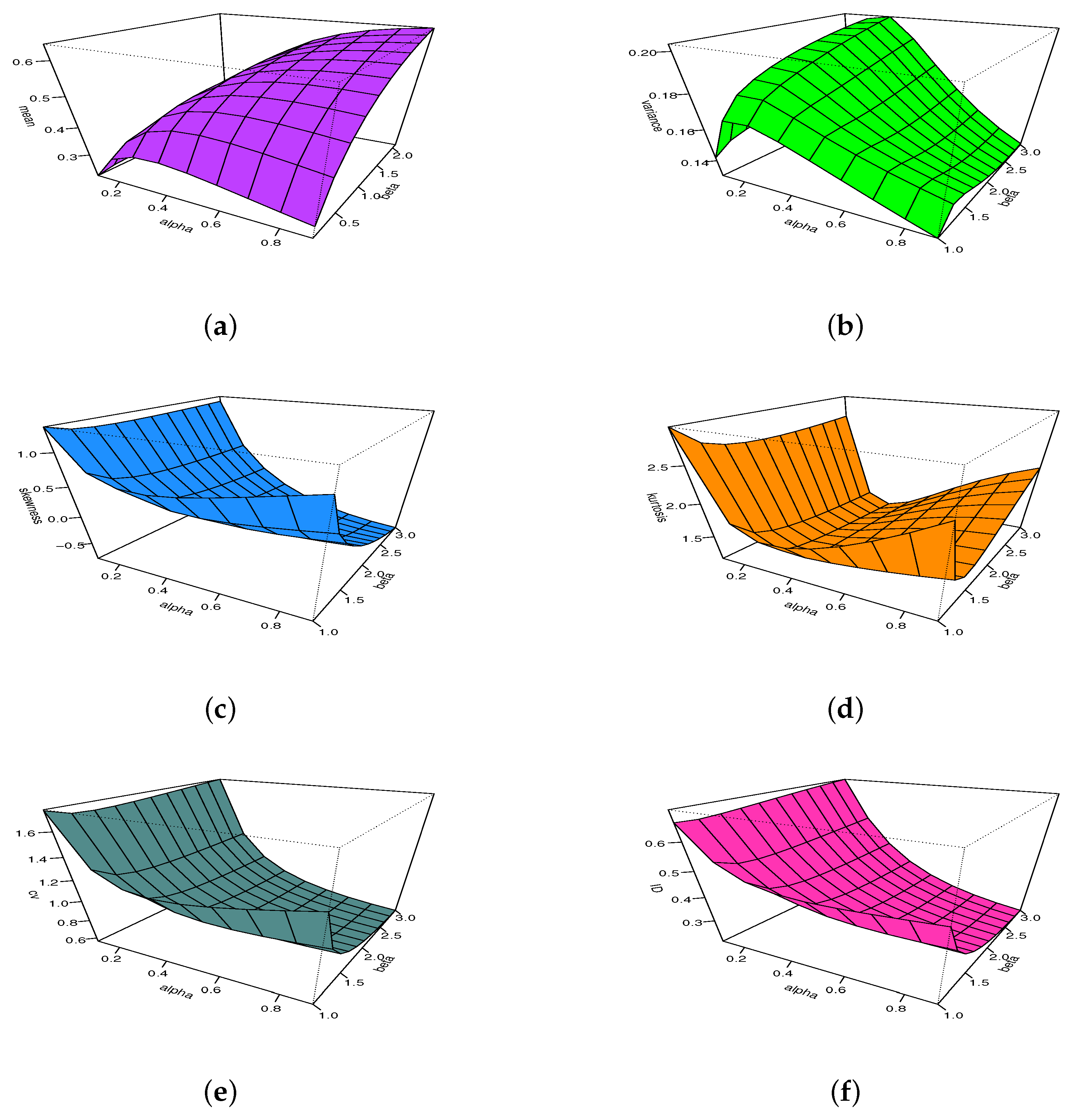
Figure 8.
The 3D plots of the (a) mean, (b) variance, (c) moment skewness, (d) moment kurtosis, (e) coefficient of variation and (f) index of dispersion for the MKw distribution for and .
Figure 8.
The 3D plots of the (a) mean, (b) variance, (c) moment skewness, (d) moment kurtosis, (e) coefficient of variation and (f) index of dispersion for the MKw distribution for and .
Figure 9.
Plots of the (a) estimated pdfs and (b) estimated cdfs over the appropriate statistical objects for the maximum flood level data set.
Figure 9.
Plots of the (a) estimated pdfs and (b) estimated cdfs over the appropriate statistical objects for the maximum flood level data set.
Figure 10.
Plots of the (a) estimated pdfs and (b) estimated cdfs over the appropriate statistical objects for the air conditioning system data set.
Figure 10.
Plots of the (a) estimated pdfs and (b) estimated cdfs over the appropriate statistical objects for the air conditioning system data set.
Table 1.
Numerical values of moment measures for a random variable X following the MKw distribution with and varying .
Table 1.
Numerical values of moment measures for a random variable X following the MKw distribution with and varying .
| | | | | Var | MS | MK | CV | ID |
|---|
| 0.5 | 0.894 | 0.835 | 0.793 | 0.76 | 0.036 | −2.736 | 11.244 | 0.213 | 0.041 |
| 1.0 | 0.838 | 0.744 | 0.679 | 0.63 | 0.042 | −1.796 | 6.393 | 0.245 | 0.05 |
| 1.5 | 0.798 | 0.676 | 0.602 | 0.545 | 0.039 | −0.032 | −6.622 | 0.248 | 0.049 |
| 2.0 | 0.762 | 0.631 | 0.543 | 0.477 | 0.05 | −1.3 | 3.891 | 0.295 | 0.066 |
| 2.5 | 0.734 | 0.587 | 0.496 | 0.428 | 0.048 | −0.534 | −0.3 | 0.298 | 0.065 |
| 3.0 | 0.711 | 0.553 | 0.458 | 0.389 | 0.048 | −0.419 | 0.127 | 0.309 | 0.068 |
| 3.5 | 0.69 | 0.525 | 0.424 | 0.357 | 0.049 | −0.483 | 2.431 | 0.32 | 0.071 |
| 4.0 | 0.672 | 0.5 | 0.397 | 0.33 | 0.049 | −0.38 | 2.341 | 0.329 | 0.073 |
| 4.5 | 0.655 | 0.478 | 0.374 | 0.308 | 0.049 | −0.292 | 2.287 | 0.337 | 0.074 |
Table 2.
Numerical values of moment measures for a random variable X following the MKw distribution with and varying .
Table 2.
Numerical values of moment measures for a random variable X following the MKw distribution with and varying .
| | | | | Var | MS | MK | CV | ID |
|---|
| 0.5 | 0.213 | 0.129 | 0.101 | 0.087 | 0.084 | 1.574 | 4.215 | 1.357 | 0.393 |
| 1.0 | 0.354 | 0.213 | 0.156 | 0.129 | 0.087 | 0.729 | 2.727 | 0.834 | 0.247 |
| 1.5 | 0.459 | 0.288 | 0.211 | 0.172 | 0.077 | 0.387 | 2.428 | 0.604 | 0.168 |
| 2.0 | 0.537 | 0.354 | 0.264 | 0.211 | 0.066 | 0.133 | 2.036 | 0.48 | 0.124 |
| 2.5 | 0.595 | 0.411 | 0.311 | 0.251 | 0.057 | −0.084 | 2.195 | 0.401 | 0.096 |
| 3.0 | 0.641 | 0.459 | 0.354 | 0.288 | 0.049 | −0.215 | 2.258 | 0.345 | 0.076 |
| 3.5 | 0.677 | 0.501 | 0.393 | 0.323 | 0.042 | −0.377 | 2.749 | 0.303 | 0.062 |
| 4.0 | 0.707 | 0.537 | 0.428 | 0.354 | 0.037 | −0.503 | 2.951 | 0.272 | 0.052 |
| 4.5 | 0.732 | 0.568 | 0.459 | 0.384 | 0.032 | −0.625 | 3.349 | 0.246 | 0.044 |
Table 3.
Numerical values of the MLLEs, MSErs, CoI-LBs, CoI-UBs, and CoI-LENs for ( = 0.5, = 0.5) of the MKw model.
Table 3.
Numerical values of the MLLEs, MSErs, CoI-LBs, CoI-UBs, and CoI-LENs for ( = 0.5, = 0.5) of the MKw model.
| n | MLLE | MSEr | 90% | 95% |
|---|
| CoI-LB | CoI-UB | CoI-LEN | CoI-LB | CoI-UB | CoI-LEN |
|---|
| 30 | 1.6622 | 0.3629 | 0.9792 | 2.3451 | 1.3659 | 0.8485 | 2.4759 | 1.6274 |
| | 0.5311 | 0.0223 | 0.3457 | 0.7165 | 0.3708 | 0.3102 | 0.7520 | 0.4418 |
| 50 | 1.6082 | 0.1195 | 1.1166 | 2.0998 | 0.9833 | 1.0224 | 2.1940 | 1.1716 |
| | 0.5268 | 0.0111 | 0.3848 | 0.6688 | 0.2840 | 0.3576 | 0.6960 | 0.3384 |
| 100 | 1.5114 | 0.0382 | 1.1943 | 1.8284 | 0.6341 | 1.1336 | 1.8891 | 0.7555 |
| | 0.4998 | 0.0037 | 0.4037 | 0.5958 | 0.1922 | 0.3853 | 0.6142 | 0.2290 |
| 200 | 1.5141 | 0.0180 | 1.2896 | 1.7386 | 0.4490 | 1.2466 | 1.7816 | 0.5350 |
| | 0.5015 | 0.0018 | 0.4333 | 0.5697 | 0.1364 | 0.4203 | 0.5828 | 0.1625 |
| 500 | 1.4992 | 0.0060 | 1.3593 | 1.6392 | 0.2799 | 1.3325 | 1.6660 | 0.3335 |
| | 0.4991 | 0.0006 | 0.4561 | 0.5421 | 0.0860 | 0.4479 | 0.5503 | 0.1024 |
| 1000 | 1.5151 | 0.0039 | 1.4146 | 1.6155 | 0.2009 | 1.3954 | 1.6348 | 0.2394 |
| | 0.5042 | 0.0004 | 0.4735 | 0.5348 | 0.0613 | 0.4677 | 0.5407 | 0.0731 |
Table 4.
Numerical values of the MLLEs, MSErs, CoI-LBs, CoI-UBs, and CoI-LENs for ( = 0.5, = 1.2) of the MKw model.
Table 4.
Numerical values of the MLLEs, MSErs, CoI-LBs, CoI-UBs, and CoI-LENs for ( = 0.5, = 1.2) of the MKw model.
| n | MLLE | MSEr | 90% | 95% |
|---|
| CoI-LB | CoI-UB | CoI-LEN | CoI-LB | CoI-UB | CoI-LEN |
|---|
| 30 | 0.5485 | 0.0109 | 0.3935 | 0.7034 | 0.3099 | 0.3639 | 0.7331 | 0.3692 |
| | 1.3745 | 0.1687 | 0.7487 | 2.0004 | 1.2517 | 0.6288 | 2.1202 | 1.4914 |
| 50 | 0.5303 | 0.0073 | 0.4167 | 0.6439 | 0.2273 | 0.3949 | 0.6657 | 0.2708 |
| | 1.3645 | 0.1538 | 0.8800 | 1.8489 | 0.9690 | 0.7872 | 1.9417 | 1.1545 |
| 100 | 0.5125 | 0.0023 | 0.4354 | 0.5896 | 0.1541 | 0.4207 | 0.6043 | 0.1836 |
| | 1.2505 | 0.0428 | 0.9322 | 1.5687 | 0.6365 | 0.8713 | 1.6297 | 0.7583 |
| 200 | 0.5038 | 0.0011 | 0.4508 | 0.5569 | 0.1062 | 0.4406 | 0.5671 | 0.1265 |
| | 1.2282 | 0.0216 | 1.0060 | 1.4504 | 0.4444 | 0.9634 | 1.4929 | 0.5295 |
| 500 | 0.4973 | 0.0005 | 0.4644 | 0.5302 | 0.0658 | 0.4581 | 0.5365 | 0.0784 |
| | 1.1947 | 0.0099 | 1.0575 | 1.3319 | 0.2744 | 1.0313 | 1.3582 | 0.3269 |
| 1000 | 0.4999 | 0.0002 | 0.4765 | 0.5233 | 0.0469 | 0.4720 | 0.5278 | 0.0558 |
| | 1.2039 | 0.0027 | 1.1062 | 1.3015 | 0.1953 | 1.0875 | 1.3202 | 0.2326 |
Table 5.
Numerical values of the MLLEs, MSErs, CoI-LBs, CoI-UBs, and CoI-LENs for ( = 1.2, = 0.5) of the MKw model.
Table 5.
Numerical values of the MLLEs, MSErs, CoI-LBs, CoI-UBs, and CoI-LENs for ( = 1.2, = 0.5) of the MKw model.
| n | MLLE | MSEr | 90% | 95% |
|---|
| CoI-LB | CoI-UB | CoI-LEN | CoI-LB | CoI-UB | CoI-LEN |
|---|
| 30 | 1.2612 | 0.0859 | 0.8003 | 1.7221 | 0.9218 | 0.7120 | 1.8104 | 1.0983 |
| | 0.4939 | 0.0137 | 0.3132 | 0.6746 | 0.3613 | 0.2786 | 0.7092 | 0.4305 |
| 50 | 1.2505 | 0.0858 | 0.8961 | 1.6048 | 0.7087 | 0.8283 | 1.6727 | 0.8444 |
| | 0.5147 | 0.0131 | 0.3683 | 0.6610 | 0.2927 | 0.3403 | 0.6891 | 0.3487 |
| 100 | 1.2547 | 0.0323 | 1.0054 | 1.5041 | 0.4987 | 0.9577 | 1.5518 | 0.5941 |
| | 0.5182 | 0.0049 | 0.4143 | 0.6222 | 0.2079 | 0.3944 | 0.6421 | 0.2477 |
| 200 | 1.2206 | 0.0099 | 1.0516 | 1.3896 | 0.3380 | 1.0192 | 1.4219 | 0.4028 |
| | 0.5035 | 0.0014 | 0.4318 | 0.5752 | 0.1433 | 0.4181 | 0.5889 | 0.1708 |
| 500 | 1.2091 | 0.0050 | 1.1037 | 1.3145 | 0.2107 | 1.0835 | 1.3346 | 0.2511 |
| | 0.5035 | 0.0007 | 0.4581 | 0.5489 | 0.0908 | 0.4494 | 0.5576 | 0.1082 |
| 1000 | 1.2081 | 0.0015 | 1.1338 | 1.2824 | 0.1486 | 1.1196 | 1.2967 | 0.1771 |
| | 0.5055 | 0.0004 | 0.4733 | 0.5377 | 0.0644 | 0.4671 | 0.5439 | 0.0768 |
Table 6.
Numerical values of the MLLEs, MSErs, CoI-LBs, CoI-UBs, and CoI-LENs for ( = 0.8, = 0.5) of the MKw model.
Table 6.
Numerical values of the MLLEs, MSErs, CoI-LBs, CoI-UBs, and CoI-LENs for ( = 0.8, = 0.5) of the MKw model.
| n | MLLE | MSEr | 90% | 95% |
|---|
| CoI-LB | CoI-UB | CoI-LEN | CoI-LB | CoI-UB | CoI-LEN |
|---|
| 30 | 0.8409 | 0.0326 | 0.5709 | 1.1109 | 0.5400 | 0.5192 | 1.1626 | 0.6434 |
| | 0.5234 | 0.0217 | 0.3126 | 0.7342 | 0.4216 | 0.2722 | 0.7746 | 0.5024 |
| 50 | 0.8634 | 0.0248 | 0.6475 | 1.0793 | 0.4318 | 0.6062 | 1.1206 | 0.5144 |
| | 0.5526 | 0.0157 | 0.3816 | 0.7235 | 0.3419 | 0.3489 | 0.7562 | 0.4073 |
| 100 | 0.8432 | 0.0083 | 0.6963 | 0.9901 | 0.2938 | 0.6681 | 1.0182 | 0.3501 |
| | 0.5268 | 0.0048 | 0.4109 | 0.6428 | 0.2319 | 0.3887 | 0.6650 | 0.2764 |
| 200 | 0.8118 | 0.0024 | 0.7046 | 0.8989 | 0.1943 | 0.6860 | 0.9175 | 0.2315 |
| | 0.5074 | 0.0016 | 0.4273 | 0.5875 | 0.1601 | 0.4120 | 0.6028 | 0.1908 |
| 500 | 0.8038 | 0.0020 | 0.7559 | 0.8817 | 0.1258 | 0.7439 | 0.8938 | 0.1499 |
| | 0.5098 | 0.0015 | 0.4593 | 0.5603 | 0.1010 | 0.4496 | 0.5699 | 0.1203 |
| 1000 | 0.8023 | 0.0009 | 0.7589 | 0.8456 | 0.0867 | 0.7506 | 0.8539 | 0.1033 |
| | 0.5011 | 0.0004 | 0.4658 | 0.5363 | 0.0706 | 0.4590 | 0.5431 | 0.0841 |
Table 7.
Numerical values of the MLLEs, MSErs, CoI-LBs, CoI-UBs, and CoI-LENs for ( = 0.8, = 0.8) of the MKw model.
Table 7.
Numerical values of the MLLEs, MSErs, CoI-LBs, CoI-UBs, and CoI-LENs for ( = 0.8, = 0.8) of the MKw model.
| n | MLLE | MSEr | 90% | 95% |
|---|
| CoI-LB | CoI-UB | CoI-LEN | CoI-LB | CoI-UB | CoI-LEN |
|---|
| 30 | 0.8875 | 0.0505 | 0.5967 | 1.1783 | 0.5815 | 0.5411 | 1.2340 | 0.6929 |
| | 0.8732 | 0.0513 | 0.5263 | 1.2201 | 0.6939 | 0.4598 | 1.2866 | 0.8268 |
| 50 | 0.8615 | 0.0244 | 0.6491 | 1.0739 | 0.4248 | 0.6084 | 1.1146 | 0.5062 |
| | 0.8514 | 0.0345 | 0.5889 | 1.1139 | 0.5250 | 0.5386 | 1.1642 | 0.6255 |
| 100 | 0.8282 | 0.0114 | 0.6837 | 0.9726 | 0.2888 | 0.6561 | 1.0002 | 0.3441 |
| | 0.8408 | 0.0162 | 0.6545 | 1.0271 | 0.3726 | 0.6188 | 1.0628 | 0.4440 |
| 200 | 0.8035 | 0.0028 | 0.7063 | 0.9007 | 0.1943 | 0.6877 | 0.9193 | 0.2316 |
| | 0.8069 | 0.0056 | 0.6798 | 0.9340 | 0.2541 | 0.6555 | 0.9583 | 0.3028 |
| 500 | 0.8040 | 0.0014 | 0.7426 | 0.8653 | 0.1227 | 0.7309 | 0.8771 | 0.1462 |
| | 0.8033 | 0.0021 | 0.7233 | 0.8832 | 0.1599 | 0.7080 | 0.8985 | 0.1905 |
| 1000 | 0.7977 | 0.0006 | 0.7547 | 0.8407 | 0.0860 | 0.7465 | 0.8489 | 0.1024 |
| | 0.8008 | 0.0011 | 0.7443 | 0.8573 | 0.1130 | 0.7335 | 0.8681 | 0.1346 |
Table 8.
Numerical values of the MLLEs, MSErs, CoI-LBs, CoI-UBs, and CoI-LENs for ( = 0.5, = 1.5) of the MKw model.
Table 8.
Numerical values of the MLLEs, MSErs, CoI-LBs, CoI-UBs, and CoI-LENs for ( = 0.5, = 1.5) of the MKw model.
| n | MLLE | MSEr | 90% | 95% |
|---|
| CoI-LB | CoI-UB | CoI-LEN | CoI-LB | CoI-UB | CoI-LEN |
|---|
| 30 | 0.5295 | 0.0103 | 0.3812 | 0.6777 | 0.2965 | 0.3529 | 0.7061 | 0.3532 |
| | 1.7019 | 0.3967 | 0.9201 | 2.4837 | 1.5636 | 0.7704 | 2.6334 | 1.8630 |
| 50 | 0.5269 | 0.0061 | 0.4128 | 0.6410 | 0.2282 | 0.3909 | 0.6628 | 0.2719 |
| | 1.6688 | 0.1760 | 1.0730 | 2.2646 | 1.1916 | 0.9589 | 2.3786 | 1.4197 |
| 100 | 0.5192 | 0.0026 | 0.4411 | 0.5973 | 0.1562 | 0.4262 | 0.6123 | 0.1861 |
| | 1.5894 | 0.0557 | 1.1863 | 1.9925 | 0.8063 | 1.1091 | 2.0697 | 0.9606 |
| 200 | 0.5065 | 0.0010 | 0.4531 | 0.5600 | 0.1068 | 0.4429 | 0.5702 | 0.1273 |
| | 1.5332 | 0.0327 | 1.2565 | 1.8100 | 0.5535 | 1.2035 | 1.8630 | 0.6595 |
| 500 | 0.5006 | 0.0004 | 0.4674 | 0.5339 | 0.0665 | 0.4610 | 0.5403 | 0.0792 |
| | 1.5192 | 0.0115 | 1.3450 | 1.6934 | 0.3484 | 1.3116 | 1.7267 | 0.4151 |
| 1000 | 0.4998 | 0.0002 | 0.4764 | 0.5233 | 0.0469 | 0.4719 | 0.5278 | 0.0559 |
| | 1.5007 | 0.0057 | 1.3790 | 1.6224 | 0.2434 | 1.3557 | 1.6457 | 0.2900 |
Table 9.
Numerical values of the MLLEs, MSErs, CoI-LBs, CoI-UBs, and CoI-LENs for ( = 0.5, = 2.0) of the MKw model.
Table 9.
Numerical values of the MLLEs, MSErs, CoI-LBs, CoI-UBs, and CoI-LENs for ( = 0.5, = 2.0) of the MKw model.
| n | MLLE | MSEr | 90% | 95% |
|---|
| CoI-LB | CoI-UB | CoI-LEN | CoI-LB | CoI-UB | CoI-LEN |
|---|
| 30 | 0.5206 | 0.0063 | 0.3754 | 0.6658 | 0.2904 | 0.3476 | 0.6936 | 0.3460 |
| | 2.1889 | 0.3108 | 1.1732 | 3.2046 | 2.0313 | 0.9788 | 3.3991 | 2.4203 |
| 50 | 0.5237 | 0.0043 | 0.4117 | 0.6357 | 0.2239 | 0.3903 | 0.6571 | 0.2668 |
| | 2.1641 | 0.2081 | 1.3904 | 2.9377 | 1.5474 | 1.2422 | 3.0859 | 1.8437 |
| 100 | 0.5095 | 0.0021 | 0.4334 | 0.5857 | 0.1524 | 0.4188 | 0.6003 | 0.1816 |
| | 2.0274 | 0.1227 | 1.5102 | 2.5447 | 1.0345 | 1.4111 | 2.6437 | 1.2326 |
| 200 | 0.4988 | 0.0009 | 0.4464 | 0.5512 | 0.1048 | 0.4364 | 0.5612 | 0.1248 |
| | 2.0031 | 0.0449 | 1.6395 | 2.3667 | 0.7272 | 1.5699 | 2.4363 | 0.8664 |
| 500 | 0.5019 | 0.0003 | 0.4685 | 0.5353 | 0.0668 | 0.4621 | 0.5417 | 0.0796 |
| | 1.9800 | 0.0214 | 1.7531 | 2.2070 | 0.4538 | 1.7097 | 2.2504 | 0.5407 |
| 1000 | 0.5014 | 0.0002 | 0.4778 | 0.5250 | 0.0472 | 0.4733 | 0.5296 | 0.0563 |
| | 1.9914 | 0.0072 | 1.8299 | 2.1529 | 0.3230 | 1.7990 | 2.1838 | 0.3849 |
Table 10.
Competent models with the MKw model.
Table 10.
Competent models with the MKw model.
| Models | Cdfs | References |
|---|
| TKw | | [6] |
| Kw | | [4] |
| Beta | | [1] |
| UR | | [12] |
| Topp | | [25] |
| Power | | (Classic) |
Table 11.
MLLEs and SEs of the models for the maximum flood level data set.
Table 11.
MLLEs and SEs of the models for the maximum flood level data set.
| Models | | MLLEs (SEs) | |
|---|
| MKw | 354.0108 | 5.9002 | |
| (5.0365) | (1.2035) | |
| TKw | 3.7445 | 11.1649 | 0.6201 |
| (0.6505) | (6.1634) | (0.3722) |
| Kw | 3.3773 | 12.0018 | |
| (0.6041) | (5.4713) | |
| Beta | 6.8309 | 9.2364 | |
| (2.1179) | (2.8912) | |
| UR | 1.1366 | | |
| (0.2541) | | |
| Topp | 2.2412 | | |
| (0.5011) | | |
| Power | 1.7804 | | |
| (0.2487) | | |
Table 12.
Values of , AIC, W, A, KS and (KS p-value) of the models for the maximum flood level data set.
Table 12.
Values of , AIC, W, A, KS and (KS p-value) of the models for the maximum flood level data set.
| Models | | AIC | W | A | KS | p-Value |
|---|
| MKw | −15.7652 | −27.5305 | 0.0437 | 0.2959 | 0.1143 | 0.9562 |
| TKw | −13.6401 | −21.2802 | 0.1420 | 0.8417 | 0.2001 | 0.3993 |
| Kw | −12.9732 | −21.9465 | 0.1672 | 0.9746 | 0.2175 | 0.3004 |
| Beta | −14.18350 | −24.3671 | 0.1267 | 0.7514 | 0.2062 | 0.3625 |
| UR | −11.1176 | −20.2352 | 0.0892 | 0.5367 | 0.2892 | 0.0704 |
| Topp | −7.3813 | −12.7627 | 0.1194 | 0.7110 | 0.3409 | 0.0191 |
| Power | −0.1097 | 1.7804 | 0.1229 | 0.7300 | 0.3977 | 0.0035 |
Table 13.
MLLEs and SEs of the models for the air conditioning system data set.
Table 13.
MLLEs and SEs of the models for the air conditioning system data set.
| Models | MLLEs (SEs) | | |
|---|
| MKw | 11.6229 | 0.9719 | |
| (1.8815) | (0.1868) | |
| TKw | 0.6274 | 1.1217 | 0.6622 |
| (0.1245) | (0.3444) | (0.2631) |
| Kw | 0.5451 | 1.3837 | |
| (0.1148) | (0.3361) | |
| Beta | 0.5141 | 1.3429 | |
| (0.1118) | (0.3642) | |
| UR | 0.1497 | | |
| (0.0273) | | |
| Topp | 0.6017 | | |
| (0.1098) | | |
| Power | 0.4501 | | |
| (0.0821) | | |
Table 14.
Values of , AIC, W, A, KS and (KS p-value) of the models for the air conditioning system data set.
Table 14.
Values of , AIC, W, A, KS and (KS p-value) of the models for the air conditioning system data set.
| Models | | AIC | W | A | KS | p-Value |
|---|
| MKw | −17.8873 | −31.7747 | 0.0929 | 0.4899 | 0.1261 | 0.7260 |
| TKw | −14.9975 | −23.9950 | 0.1691 | 1.0856 | 0.1744 | 0.3210 |
| Kw | −13.5389 | −23.0778 | 0.2109 | 1.3470 | 0.1878 | 0.2403 |
| Beta | −13.2463 | −22.49261 | 0.2173 | 1.3858 | 0.1957 | 0.2003 |
| UR | −12.7730 | −23.5461 | 0.1253 | 0.7933 | 0.1314 | 0.6776 |
| Topp | −11.9801 | −21.9603 | 0.2379 | 1.5102 | 0.1938 | 0.2095 |
| Power | −12.7018 | −23.4036 | 0.2068 | 1.3212 | 0.2031 | 0.1680 |


 ,
, 


