Overview in Summabilities: Summation Methods for Divergent Series, Ramanujan Summation and Fractional Finite Sums

Abstract

This work presents an overview of the summability of divergent series and fractional finite sums, including their connections. Several summation methods listed, including the smoothed sum, permit obtaining an algebraic constant related to a divergent series. The first goal is to revisit the discussion about the existence of an algebraic constant related to a divergent series, which does not contradict the divergence of the series in the classical sense. The well-known Euler–Maclaurin summation formula is presented as an important tool. Throughout a systematic discussion, we seek to promote the Ramanujan summation method for divergent series and the methods recently developed for fractional finite sums.

1. Introduction

The sum was probably the first mathematical operation that humans performed and abstracted, and the properties of finite sums are well known. The symbol used to shortly represent a sum is due to L. Euler, who introduced the symbol $\sum$. Indeed, in 1755, he wrote: “summam indicabimus signo $\sum$”, which means, we indicate a sum with the sign $\sum$ [1,2,3]. This succinct notation, known as sigma notation, was rarely used for some time. A.-L. Cauchy, in his celebrated Cours D’Analyse of 1821 [4,5], used sums in the expanded form. The sigma notation started to spread after being adopted by J.-B. Fourier in 1822 to express sums [3,6].

The expression ${\sum }_{k=1}^{n}f\left(k\right)$ is used to shortly indicate a sum that has exactly the terms $f\left(k\right)$ with index k covering all integers between, including the limits 1 and n [7]. The sigma notation is a compact notation with properties that simplify algebraic operations [7,8] and is suitable for denoting sums with an infinite number of terms. For infinite sums, called series, the currently used definition is due to Cauchy [4,5], who also introduced the definition of convergent and divergent series. The concepts about series, as well as the conditions of convergence in the classical sense (i.e., in the Cauchy’s sense), are today well established, and the meaning of sequences, partial sums, and the convergence and divergence of sequences and series are included in many textbooks used in undergraduate courses.

Classically, when someone analyzes a series, the first question is “Is this series convergent? (in the classical sense)”. If the series is convergent, then the second question is “To which value does the series converge?”. According to Cauchy, if a series does not converge in the classical sense, then it is divergent. Two types of divergent series are possible: those that grow in absolute value without limit, and those that are bounded but whose sequence of partial sums does not approximate any specific value (eventually oscillates infinitely). When a given series is divergent in the classical sense, a third question arises: “Is it still possible to obtain any useful information from this series?”. The answer to this question can be “yes”, provided an adequate summation method (SM) is used.

The objectives of this manuscript are (i) to present several SM that allow the extracting of a single algebraic constant related to each divergent series, including the smoothed sum method [9]; (ii) to solve some discrepancies about the use and correctness of these SM, including the Ramanujan summation [10,11,12]; and (iii) to illustrate the concept of fractional finite sums [13,14,15,16] and their associated techniques of applicability.

This manuscript is organized as follows: Section 2 gives fundamental concepts of divergent series and introduces several methods of summability that allow obtaining specific and useful information, namely an algebraic constant related to each divergent series, including the smoothed sums method. Section 3 covers the Ramanujan summation, including the concept of the Ramanujan coefficient of a series. Section 4 discusses topics related to the concept of fractional finite sums and introduces recent methods developed for their evaluation. Section 5 draws some connections between these summability theories. Section 6 is dedicated to some conclusions. Figure 1 presents a mind map of the structure of summability theories, including the names of the main contributors to each covered theory and the years of the registered contributions.

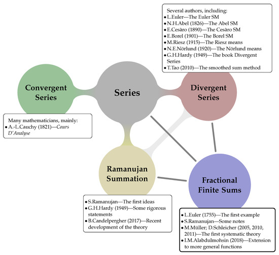
Figure 1. Mind map of the structure. Lists of the main contributors/year of contribution.

Remark 1.

To help avoid misunderstanding with the summation methods and their notations throughout this overview, we introduce the following form for denoting a sum: when the sum is considered in the classical sense, we only use the symbol ∑, but to represent another specific SM, we include left superscript letters. For example, the symbol ${}^{\mathcal{A}b}\sum$ is written to specify that the sum is in the Abel sense.

Remark 2.

In this manuscript, we only deal with SM in the context of Archimedean algebra. An example of summability theory in non-Archimedean algebra [17] is the ultrametric summability theory [18], which uses general matrix transformations in the ultrametric analysis [19,20]. Sometimes, the summation methods that use matrices are attributed to Andree and Petersen [21], who gave conditions for matrices to have properties of convergence similar to those of sequences, but the topic was discussed previously by Hardy [22]. Interested readers can find more information about matrix methods of summation in [23,24,25,26]. Ultrametric summability theory and matrix methods of summations are not covered in this manuscript.

2. Divergent Series and Summation Formulae

Before recalling the definition of a divergent series, it is convenient to mention the definitions of series and convergent series. The current concept of series and convergent series is due to Cauchy [4,5], who considered a series as a sequence of values $a_0,a_1,a_2,\cdots$ derived from each other according to a known law. Cauchy considered the sequence ${\left(s_n\right)}_{n\in \mathbb{N}}$ of the sums of the nth initial terms of the sequence ${\left(a_n\right)}_{n\in \mathbb{N}}$ described by

$$s_n=a_0+a_1+\cdots +a_n.$$

(1)

He stated that an infinite series ${\sum }_{n=0}^{\infty }{a}_n$ is convergent if the limit of partial sums $s_n$ exists and is equal to one well-determined numeric value s.

When a given series is convergent in Cauchy’s sense, it is written ${\sum }_{n=0}^{\infty }{a}_n=s$, and s is considered the sum in the classical sense of the series. Still, according to Cauchy, when a given series is not convergent, it is said to be divergent.

The existence of one algebraic constant related to a divergent series is naturally related to its asymptotic expansion and does not contradict the fact that such a series diverges in the classical sense. In the following section, we present the general requirements for an SM to make sense. We also list several SM, which in many cases allow one to obtain one single algebraic constant related to a given series, usually mentioned as “the sum” of the series.

2.1. About a General Summation Method

According to Hardy [22], the development of the theory of divergent series is based on adequate generalizations of the limit of a sequence. Usually, an auxiliary sequence of linear means of the partial sum $s_n$ is used.

We say that two SM are consistent with each other when a given series has the same sum by both methods [22]. Between two consistent SM, the strongest is the one that can sum more series, i.e., the stronger method includes the other one [16,22].

An SM should have the properties: (i) regularity, which occurs when the value assigned to a series by the SM agrees with its sum in the classical sense [16,22,27]; (ii) linearity, when for $\alpha ,\beta \in \mathbb{C}$, we have [12,22,27]

$${\displaystyle \sum _{n=0}^{\infty }(\alpha a_n+\beta b_n)=\alpha \sum _{n=0}^{\infty }{a}_n+\beta \sum _{n=0}^{\infty }{b}_n;}$$

(2)

(iii) range property [27], that is, the method can attribute a specific numeric value to at least one divergent series; and (iv) stability, when the method presents the classical translation property [12,16]:

$${\displaystyle \sum _{n=0}^{\infty }{a}_n=a_0+\sum _{n=0}^{\infty }{a}_{n+1}.}$$

(3)

However, according to Candelpergher [12], we must not consider this property if we adopt other definitions of summation procedures, in addition to the traditional limit of partial sums (see Section 3).

According to Hardy [22], we can use any linear transformation $\mathcal{T}$, of the averages type, to define a procedure that aims at the summation of series, and classical methods of summation that use means of partial sums can be summarized as follows [12,22].

Let us consider $\mathcal{T}$ a topological space and l an accumulation point of $\mathcal{T}$ (if $\mathcal{T}=\mathbb{N}$, then $l=+\infty$, and if $\mathcal{T}=[0,1)$, then $l=1$). Moreover, let ${\left(p_n\left(t\right)\right)}_{n\in \mathbb{N}}$ be a family of sequences satisfying the convergence of the series ${\sum }_{n=0}^{\infty }{p}_n\left(t\right)$ for all $t\in \mathcal{T}$. Then, a $\mathcal{T}$-SM can be defined by

$${\displaystyle {}^{\mathcal{T}}\sum _{n=0}^{\infty }{a}_n=\underset{t\to l}{lim}\frac{{\displaystyle \sum _{n=0}^{\infty }{p}_n\left(t\right)s_n}}{{\displaystyle \sum _{n=0}^{\infty }{p}_n\left(t\right)}},}$$

(4)

when such a limit exists, the series ${\sum }_{n=0}^{\infty }{a}_n$ is said $\mathcal{T}$-summable. These general summation methods are linear and present the classical translation property. In [22], Hardy established the necessary and sufficient conditions about the sequences ${\left(p_n\left(t\right)\right)}_{n\in \mathbb{N}}$, so that a general method coincides with the classical sum when we consider a convergent series ${\sum }_{n=0}^{\infty }{a}_n$.

2.2. The Cesàro Summation Method

The Cesàro SM, or the Cesàro means, is the first systematic and coherent averaging process for evaluating the sum of divergent series [22,28]. For a series ${\sum }_{n=0}^{\infty }{a}_n$, the Cesàro mean (of first order) is defined by [22,27,29]

$${\displaystyle {}^{{\mathcal{C}e}_{\left(1\right)}}\sum _{n=0}^{\infty }{a}_n=\underset{n\to \infty }{lim}\left(\frac{1}{n+1}\sum _{k=0}^n{s}_k\right)=\underset{n\to \infty }{lim}\left(\frac{s_0+s_1+s_2+\cdots +s_n}{n+1}\right),}$$

(5)

when such a limit exists. For convergent series, if the sequence of partial sums ${\left(s_n\right)}_{n\in \mathbb{N}}$ has a limit s when $n\to \infty$, the Cesàro mean ${}^{\mathcal{C}e}{\sum }_{n=0}^{\infty }{a}_n$ must have the same limit. The Cesàro means have the properties of regularity, linearity, and stability [22], and have applicability, for example, in Fourier series [30,31,32].

It is possible to consider the Cesàro means of superior orders [22,29]. For $m>1$, if we denote the partial sums of $m\mathrm{th}$ order of the series ${\sum }_{n=0}^{\infty }{a}_n$ by $s_n^{\left(m\right)}=s_0^{(m-1)}+s_1^{(m-1)}+s_2^{(m-1)}+\cdots +s_n^{(m-1)}$, then we can write

$${\displaystyle {}^{{\mathcal{C}e}_{\left(m\right)}}\sum _{n=0}^{\infty }{a}_n=\underset{n\to \infty }{lim}\left(\frac{1}{n+1}\sum _{k=0}^n{s}_k^{(m-1)}\right),}$$

(6)

or, expressing them in terms of $a_k$, we have

$${\displaystyle {}^{{\mathcal{C}e}_{\left(m\right)}}\sum _{n=0}^{\infty }{a}_n=\underset{n\to \infty }{lim}\left(\frac{m!}{{(n+1)}^m}\sum _{k=0}^n\left(\genfrac{}{}{0pt}{}{n-k+m}{m}\right)a_k\right).}$$

(7)

The Cesàro means and the Hölder arithmetic means of $m\mathrm{th}$ order have similar definitions [22,33]. The difference is that the Cesàro means of order m have only one division, contrary to the m divisions in the Hölder mean of order m, one at each step [22]. A series ${\sum }_{n=0}^{\infty }{a}_n$ is Hölder summable to a value s, of order m, when the following limit exists:

$${\displaystyle {}^{{\mathcal{H}o}_{\left(m\right)}}\sum _{n=0}^{\infty }{a}_n=\underset{n\to \infty }{lim}{s}_n^{\left(m\right)}=\underset{n\to \infty }{lim}\left(\frac{s_0^{(m-1)}+s_1^{(m-1)}+\cdots +s_n^{(m-1)}}{n+1}\right)=s.}$$

(8)

The Cesàro means can also be defined for noninteger orders [22,34]. If $r>-1$, then defining the partial sums of noninteger r-order of the series ${\sum }_{n=0}^{\infty }{a}_n$ by

$${\displaystyle s_n^{\left(r\right)}=\sum _{k=0}^n\left(\genfrac{}{}{0pt}{}{n-k+r}{r}\right)a_k=\sum _{k=0}^n\frac{\mathsf{\Gamma }(n-k+r+1)}{\mathsf{\Gamma }(r+1)\mathsf{\Gamma }(n-k+1)}{a}_k,}$$

(9)

where $\mathsf{\Gamma }$ is the gamma function [35,36]. Observing that the asymptotic approximation $\left(\genfrac{}{}{0pt}{}{n+r}{r}\right)\sim n^r/r!$ remains valid for nonintegers arguments r, that is, with the expression [22]

$${\displaystyle \frac{\mathsf{\Gamma }(n+r+1)}{\mathsf{\Gamma }(r+1)\mathsf{\Gamma }(n+1)}\sim \frac{n^r}{\mathsf{\Gamma }(r+1)}}$$

(10)

holding, then the Cesàro means of order r can be defined by

$${\displaystyle {}^{{\mathcal{C}e}_{\left(r\right)}}\sum _{n=0}^{\infty }{a}_n=\underset{n\to \infty }{lim}\left(\frac{\mathsf{\Gamma }(r+1)}{n^r}\sum _{k=0}^n\left(\genfrac{}{}{0pt}{}{n-k+r}{r}\right)a_k\right),}$$

(11)

when such a limit exists.

2.3. The Nörlund Means

Considering a sequence $\left(p_n\right)$ of positive terms that satisfies

$${\displaystyle \frac{p_n}{{\sum }_{k=0}^n{p}_k}\to 0,}$$

(12)

the Nörlund means of a series ${\sum }_{n=0}^{\infty }{a}_n$ can be defined by [22,37,38]

$${\displaystyle {}^{\mathcal{N}o}\sum _{n=0}^{\infty }{a}_n=\underset{n\to \infty }{lim}\left(\frac{p_n{a}_0+p_{n-1}{a}_1+\cdots +p_0{a}_n}{{\sum }_{k=0}^n{p}_k}\right),}$$

(13)

when such a limit exists. A particular case of the Nörlund definition are the Hutton means [22]:

$${\displaystyle {}^{\mathcal{H}u}\sum _{n=0}^{\infty }{a}_n=\underset{n\to \infty }{lim}\frac{{\displaystyle s_{n-1}+s_n}}{2}.}$$

(14)

The Nörlund means can be seen as a generalization for the Cesàro means. If $p_n=1$ for all n, then the Nörlund means coincide with the Cesàro means of first order. If $k>0$ and if

$$p_n=\left(\genfrac{}{}{0pt}{}{n+k-1}{k-1}\right)=\frac{\mathsf{\Gamma }(n+k)}{\mathsf{\Gamma }\left(k\right)\mathsf{\Gamma }(n+1)},$$

(15)

then the Nörlund means coincides with the Cesàro means of order k [22].

2.4. The Abel Summation Method

For an increasing sequence ${\left({\lambda }_n\right)}_{n\in \mathbb{N}}$ of non-negative terms, if the series ${\sum }_{n=0}^{\infty }{a}_n{\left(e^{-x}\right)}^{{\lambda }_n}$ is convergent for all $x>0$, then the series ${\sum }_{n=0}^{\infty }{a}_n$ is Abel summable [22,39], and we write

$${}^{\mathcal{A}b}\sum _{n=0}^{\infty }{a}_n=\underset{x\to 0^{+}}{lim}\sum _{n=0}^{\infty }{a}_n{\left(e^{-x}\right)}^{{\lambda }_n},$$

(16)

when this limit exists. In the case ${\lambda }_n=n$, the known formula

$${\displaystyle {}^{\mathcal{A}b}\sum _{n=0}^{\infty }{a}_n=\underset{x\to 1^{-}}{lim}\sum _{n=0}^{\infty }{a}_n{x}^n}$$

(17)

is recovered [16,22].

A particular case of the Abel SM, where ${\lambda }_0=0$ and ${\lambda }_n=nlog\left(n\right)$ for $n\ge 1$, is the Lindelöf SM, defined by

$${\displaystyle {}^{\mathcal{L}i}\sum _{n=0}^{\infty }{a}_n=\underset{x\to 0^{+}}{lim}\sum _{n=0}^{\infty }{a}_n{n}^{-xn},}$$

(18)

when such a limit exists [16,22,40]. The Mittag-Leffler SM [22,41] is similar to the Lindelöf one, but is not a particular case of the Abel SM. The Abel SM can assign a value for a larger number of series than the Nörlund means [16,22], but is weaker than the Lambert method, defined by

$${\displaystyle {}^{\mathcal{L}a}\sum _{n=0}^{\infty }{a}_n=\underset{y\to 0^{+}}{lim}\sum _{n=0}^{\infty }{a}_n\frac{ny{\left(e^{-y}\right)}^n}{1-{\left(e^{-y}\right)}^n},}$$

(19)

when such a limit exists [22].

When a series converges in the Cesàro sense, then it also converges in the Abel sense to the same limit [42,43]. An interesting example of a series that converges in the classical sense, but is not Abel summable, is given in [44]. In physics, the Abel SM is known as adiabatic regularization [45].

2.5. The Euler Summation Method

The simplest form of an SM due to Euler emerged from Euler’s work with power series of the type ${\sum }_{n=0}^{\infty }{a}_n{x}^n$ [22,46,47]. In a similar way to the Abel SM, Euler considered the function $f\left(x\right)={\sum }_{n=0}^{\infty }{a}_n{x}^n$ of complex variable, regular in an open set containing the origin and the point $z=1$, and considered $f\left(1\right)=s$ the sum of the series. If the limit s exists when $x\to 1$, then s is the sum of the series in the Euler sense. Considering $a_n=2^n$ in this context, it is relevant the identity $(1-2x)(1+2x+4x^2+8x^3+\cdots )=1$, valid for all x. This leads to ${\displaystyle f\left(x\right)=1+2x+4x^2+8x^3\cdots =\frac{1}{1-2x}}$, which results in ${\displaystyle {}^{\mathcal{E}u}\sum _{n=0}^{\infty }{2}^n=-1}$ when $x\to 1$. The generalized Euler SM, depending on q, is derived after multiplying $f\left(x\right)$ by x. Let us suppose that the series ${\sum }_{n=0}^{\infty }{a}_n{x}^{n+1}$ converges for x small. The series ${\sum }_{n=0}^{\infty }{a}_n$ is Euler summable for all $q>0$, and we write

$${\displaystyle {}^{{\mathcal{E}u}_{\left(q\right)}}\sum _{n=0}^{\infty }{a}_n=\sum _{n=0}^{\infty }\frac{1}{{(q+1)}^{n+1}}\sum _{k=0}^n\left(\genfrac{}{}{0pt}{}{n}{k}\right)q^{n-k}{a}_k,}$$

(20)

if the last series is convergent [22]. For $q=1$, the known formula

$${\displaystyle {}^{\mathcal{E}{u}_{\left(1\right)}}\sum _{n=0}^{\infty }{a}_n=\sum _{n=0}^{\infty }\frac{1}{2^{n+1}}\sum _{k=0}^n\left(\genfrac{}{}{0pt}{}{n}{k}\right)a_k}$$

(21)

is recovered, and for $q=0$, we obtain the sum in the classical sense [22]. For alternating series, where $a_n={(-1)}^{n-1}g\left(n\right)$, the Euler summation formula is given by [12,16]

$${\displaystyle {}^{\mathcal{E}{u}_{\left(1\right)}}\sum _{n=0}^{\infty }{a}_n=\sum _{n=0}^{\infty }\frac{{(-1)}^n}{2^{n+1}}\sum _{k=0}^n\left(\genfrac{}{}{0pt}{}{n}{k}\right){(-1)}^{n-k}g\left(k\right).}$$

(22)

2.6. The Borel Summation Methods

For a series ${\sum }_{n=0}^{\infty }{a}_n$ of complex numbers with partial sums given by $s_n={\sum }_{k=0}^n{a}_k$ (and with $s_0=0$), supposing that the series ${\displaystyle \sum _{n=0}^{\infty }\frac{t^n}{n!}{s}_n}$ is convergent for every $t>0$, the weak Borel sum of the series ${\sum }_{n=0}^{\infty }{a}_n$ (exponential method) is defined by

$${\displaystyle {}^{\mathcal{B}o}\sum _{n=0}^{\infty }{a}_n=\underset{t\to +\infty }{lim}{e}^{-t}\sum _{n=0}^{\infty }\frac{t^n}{n!}{s}_n,}$$

(23)

when such a limit exists [22,48]. More generally, if a series ${\sum }_{n=0}^{\infty }{a}_n{z}^n$ of complex terms with partial sums given by ${\displaystyle s_n\left(z\right)=\sum _{k=0}^n{a}_k{z}^k}$ is such that ${\displaystyle e^{-t}\sum _{n=0}^{\infty }\frac{t^n}{n!}{s}_n\left(z\right)}$ converges, then we say that the weak Borel sum converges at $z\in \mathbb{C}$.

If the series ${\displaystyle \sum _{n=0}^{\infty }\frac{t^n}{n!}{s}_n}$ is convergent for every $t>0$, the function ${\displaystyle s:t\mapsto e^{-t}\sum _{n=0}^{\infty }\frac{t^n}{n!}{s}_n}$ is an entire function, and thus, the series ${\sum }_{n=0}^{\infty }{a}_n$ is Borel summable (integral method) with

$${\displaystyle {}^{\mathcal{B}o}\sum _{n=0}^{\infty }{a}_n={\int }_0^{+\infty }{e}^{-t}\left(\sum _{n=0}^{\infty }\frac{t^n}{n!}{a}_n\right)dt,}$$

(24)

if the integral is convergent. More generally, if the integral ${\displaystyle {\int }_0^{+\infty }{e}^{-t}\left(\sum _{n=0}^{\infty }\frac{t^n{z}^n}{n!}{a}_n\right)dt}$ converges, then we say that the Borel sum converges at $z\in \mathbb{C}$ [12,22].

It is important to observe that, although there is a relationship between the two Borel SM, they are not equivalent [22].

The Borel integral method is the most known process of mean defined by integral functions. Other integral methods, not included in this manuscript, are the Valiron’s method (a generalization of the Borel method) and the moment constant method [22]. The Borel SM has a wide range of applications, playing an important role in asymptotic analysis and semiclassical methods. For example, it is used in the context of Wentzel-Kramers-Brillouin (WKB) theory to find approximate solutions to certain linear differential equations [49,50,51] and in the study of the 1-D Schrödinger equation [52,53,54]. Moreover, the resurgence theory [55,56,57,58,59] is an important generalization of Borel SM.

2.7. The Riesz Means

The Riesz’s typical means are generalizations of certain types of means, concerning summable integrals [22,60]. Let us consider ${\left({\lambda }_n\right)}_{n\in \mathbb{N}}$ an increasing sequence of non-negative terms. Defining a species of analogous continuous of the partial sums of a series ${\sum }_{n=0}^{\infty }{a}_n$ by

$${\displaystyle s_{n,\lambda }\left(x\right):={\left(\sum _{k=0}^n{a}_k\right)}_{\lambda }\left(x\right)=a_0+a_1+\cdots a_n=s_n,\mathrm{for}{\lambda }_n<x\le {\lambda }_{n+1},}$$

(25)

with $s_{n,\lambda }\left(x\right)=0$ for $x\le {\lambda }_0$, for a continuous variable $\omega$ and $\mu >0$ we define

$${\displaystyle s_{\lambda }^{\left(\mu \right)}\left(\omega \right)={\left(\sum _{k=0}^n{a}_k\right)}_{\lambda }^{\left(\mu \right)}\left(\omega \right)=\frac{\mu }{{\omega }^{\mu }}{\int }_0^{\omega }{\left(\sum _{k=0}^n{a}_k\right)}_{\lambda }\left(x\right){(\omega -x)}^{\kappa -1}dx.}$$

(26)

Then, applying partial integration, we obtain

$${\displaystyle s_{n,\lambda }^{\left(\mu \right)}\left(\omega \right)={\left(\sum _{k=0}^n{a}_k\right)}_{\lambda }^{\left(\mu \right)}\left(\omega \right)=\frac{1}{{\omega }^{\mu }}{\int }_0^{\omega }{(\omega -x)}^{\mu }d{s}_{n,\lambda }\left(x\right)=\sum _{{\lambda }_k={\lambda }_0}^{\lfloor \omega \rfloor }{\left(1-\frac{{\lambda }_k}{\omega }\right)}^{\mu }{a}_k.}$$

(27)

Supposing that $s_{n,\lambda }^{\left(\mu \right)}\left(\omega \right)\to s$ when $\omega \to \infty$, the series ${\sum }_{n=0}^{\infty }{a}_n$ is Riesz summable to s, and we write

$${\displaystyle {}^{\mathcal{R}i}\sum _{n=0}^{\infty }{a}_n=\underset{\omega \to \infty }{lim}{s}_{n,\lambda }^{\left(\mu \right)}\left(\omega \right)=\underset{\omega \to \infty }{lim}\left(\sum _{{\lambda }_k={\lambda }_0}^{\lfloor \omega \rfloor }{\left(1-\frac{{\lambda }_k}{\omega }\right)}^{\mu }{a}_k\right)=s.}$$

(28)

The Riesz’s typical means are regular [22]. The Riesz arithmetic means are obtained from Equation (28) if ${\lambda }_n=n$. When ${\lambda }_n=log(n+1)$ and $\mu =1$, the Riesz mean is equivalent to the logarithmic mean [22].

2.8. Some Examples

We present some sums evaluated under specific SM for series that are divergent in the classical sense.

The Grandi’s series ${\sum }_{n=0}^{\infty }{(-1)}^n=1-1+1-1+\cdots$ is summable under several methods. As examples, we cite:

$${\displaystyle {}^{\mathcal{A}b}\sum _{n=0}^{\infty }{(-1)}^n={}^{\mathcal{E}u}\sum _{n=0}^{\infty }{(-1)}^n={}^{\mathcal{C}e}\sum _{n=0}^{\infty }{(-1)}^n={}^{\mathcal{B}o}\sum _{n=0}^{\infty }{(-1)}^n=\frac{1}{2}.}$$

(29)

The Euler alternating series ${\sum }_{n=0}^{\infty }{(-1)}^{n+1}n=1-2+3-4+\cdots$ is Abel- and Euler-summable:

$${\displaystyle {}^{\mathcal{A}b}\sum _{n=0}^{\infty }{(-1)}^{n+1}n={}^{\mathcal{E}u}\sum _{n=0}^{\infty }{(-1)}^{n+1}n=\frac{1}{4}.}$$

(30)

The geometric series with ratio 2, ${\sum }_{n=0}^{\infty }{2}^n=1+2+2^2+2^3+\cdots$, is Euler summable and

$${\displaystyle {}^{\mathcal{E}u}\sum _{n=0}^{\infty }{2}^n=-1.}$$

(31)

Even with the various SM presented in this section, many series remain not summable (or are not summable under some specific SM). As a simple example, the Euler’s series ${\sum }_{n=0}^{\infty }n$ is not Abel summable, Euler summable, or Cesàro summable.

2.9. The Euler–Maclaurin Summation Formula

The Euler-Maclaurin summation formula (EMSF) expresses a finite sum whose general term is given by a function $f\left(n\right)$, $n\in \mathbb{N}$, in terms of the integral and the derivatives of the function $f\left(x\right)$, $x\in \mathbb{R}$. The theory of this formula is more related to the asymptotic aspects of a series than with their classical sum. However, due to its importance in many branches of analysis, Hardy has dedicated the last chapter of [22] to this approach. The first entry is exactly

$${\displaystyle \sum _{m=1}^{n}f\left(m\right)\sim {\int }_a^{n}f\left(x\right)dx+C+\frac{1}{2}f\left(n\right)+\sum _{r=1}^{\infty }{(-1)}^{r-1}\frac{B_r}{\left(2r\right)!}{f}^{(2r-1)}\left(n\right),}$$

(32)

for $a\in (0,1]$, where $B_r$ are the Bernoulli numbers (Hardy did not consider the null Bernoulli numbers). For x large, the function f must have enough regularity. In addition, the derivative $f^{\left(k\right)}\left(x\right)$ must decrease when k increases. The constant $C=C_f$ in Formula (32) is called the Euler–Maclaurin constant of f [22]. More information about the Bernoulli numbers can be found in [7,61,62,63,64]. In general, Formula (32) is not an identity, but instead, it is a proximity relation.

The EMSF has this name because it was derived independently by Euler and by Maclaurin [65,66,67,68]. The idea of Euler was announced in 1732-3 and published in 1738 in [65]. Euler began to observe that to each discrete sum $S(s,n)$ of powers of integers $k^s$, it was possible to associate a continuous analogue in an integral form: the integral of the function $x^s$ of the real variable x [47]. It is clear that, in general, for a given function $f\left(x\right)$, the values for the discrete sum and for the integral are different. The question is “How do these values differ?” [47].

Many distinct ways to obtain the EMSF were proposed. One example comes from the discrete calculus given in [7], among others (see, e.g., [7,8,22,64,69,70]).

For a function $f\in C^{\infty }$, the EMSF is given by

$${\displaystyle \sum _{k=a}^{n-1}f\left(k\right)={\int }_a^{n}f\left(x\right)dx-\frac{1}{2}f\left(x\right){|}_a^n+\sum _{m=1}^{\infty }\frac{B_{2m}}{\left(2m\right)!}{f}^{(2m-1)}\left(x\right){|}_a^n,}$$

(33)

where $B_m$ are the Bernoulli numbers and $a,n\in \mathbb{N}$, with $a<n$. Note that in Formula (33), the upper limit of the sum is $n-1$, and the upper limit of the integral is n [47]. In addition, a common representation of the EMSF, with the same bound limits on the left side, is given by

$${\displaystyle \sum _{k=a}^{n}f\left(k\right)={\int }_a^{n}f\left(x\right)dx+\frac{1}{2}\left(f\left(n\right)+f\left(a\right)\right)+\sum _{m=1}^{\infty }\frac{B_{2m}}{\left(2m\right)!}{f}^{(2m-1)}\left(x\right){|}_a^n.}$$

(34)

Note that the last series in (33) or (34) can diverge, because Bernoulli numbers are present, beginning with small values, but growing fast [22].

For functions $f\left(x\right)$ that are not infinitely differentiable, but only of class $C^r$, the EMSF is given by

$${\displaystyle \sum _{k=a}^{n-1}f\left(k\right)={\int }_a^{n}f\left(x\right)dx+\left(\frac{B_1}{1!}f\left(x\right){|}_a^n+\frac{B_2}{2!}{f}^{\prime }\left(x\right){|}_a^n+\cdots +\frac{B_r}{r!}{f}^{(r-1)}\left(x\right){|}_a^n\right)+R_r.}$$

(35)

The Formula (35) includes a remainder term $R_r$, introduced by Poisson in 1823 [71]. The main task, in many situations, is precisely to evaluate the remainder term $R_r$. The exact formula for the remainder term was obtained by several authors. The following expression is due to Ka$\check{\mathrm{c}}$ [72]:

$${\displaystyle \sum _{k=a}^{n-1}f\left(k\right)={\int }_a^{n}f\left(x\right)dx+\sum _{k=1}^r\frac{B_k}{k!}\left(f^{(r-1)}\left(n\right)-f^{(r-1)}\left(a\right)\right)-{\int }_a^n\frac{{\overline{B}}_r\left(\{1-t\}\right)}{r!}{f}^{\left(r\right)}\left(t\right)dt,}$$

(36)

where ${\overline{B}}_r(·)$ are the periodic Bernoulli polynomials with index r [73], and $\left\{x\right\}$ denotes the fractional part of $x\in \mathbb{R}$, i.e., $\left\{x\right\}:=x-\lfloor x\rfloor$, with $\lfloor x\rfloor$ denoting the integer part of $x\in \mathbb{R}$.

Other summation formulae, similar to (36), are also known. Let us consider the Euler polynomials $E_n\left(x\right)$, obtained from

$${\displaystyle \frac{2e^{xt}}{e^t+1}=\sum _{n=0}^{\infty }{E}_n\left(x\right)\frac{t^n}{n!},}$$

(37)

where the Euler numbers $E_n$ are given by $E_n=2^n{E}_n(1/2)$, and the periodic Euler polynomials ${\overline{E}}_n(·)$ can be defined similarly to the periodic Bernoulli ones. The Euler-Boole summation formula (EBSF) can be defined as [74]:

$$\begin{array}{ccc}\hfill {\displaystyle \sum _{m=a}^{n-1}{(-1)}^{m}f(m+h)}& =& {\displaystyle \frac{1}{2}\sum _{k=0}^{r-1}\frac{E_k\left(h\right)}{k!}\left({(-1)}^{n-1}{f}^{\left(k\right)}\left(n\right)-{(-1)}^a{f}^{\left(k\right)}\left(a\right)\right)}\hfill \\ \hfill & & {\displaystyle +\frac{1}{2(m-1)!}{\int }_a^n{f}^{\left(r\right)}\left(x\right){\overline{E}}_{r-1}\left(\{h-x\}\right)dx,}\hfill \end{array}$$

(38)

where $h\in (0,1)$. Formula (38) is due to Boole [75] and is adequate fpr alternate series. Strodt [76] indicated a unified approach to obtain the EMSF and the EBSF, which was explored in more detail by Borwein in [74]. Other periodic generalizations for the EMSF are given, for example, by Berndt [73], Berndt and Schoenfeld [77], and Rane [78].

Hardy [22] established a relationship between the Euler–Maclaurin constant $C\left(f\right)$ that appears in Formula (32), and the Ramanujan summation (RS) of the series ${\sum }_{n=1}^{\infty }f\left(n\right)$ (denoted by Hardy as $(\mathfrak{R},a)$), and wrote

$$f\left(1\right)+f\left(2\right)+\cdots +f\left(x\right)+\cdots =C\left(f\right)(\mathfrak{R},a),$$

(39)

for $0<a\le 1$. This, apparently, gives another definition to the “sum” of a divergent series, in a different sense from previous sums recalled in this section. Hardy has chosen the symbol $\mathfrak{R}$ due to Ramanujan. In this manuscript, in order to uniformize the notation, we replace the symbol $(\mathfrak{R},a)$ by ${}^{\mathcal{R}a}{\sum }_{n=1}^{\infty }$. The RS is considered in Section 3.

2.10. The Smoothed Sum Method

In 2010, T. Tao introduced the concept of smoothed sums in his blog [79] (see also Section 3.7 of [9]) as a tool able to give an interpretation for the strange values assigned to divergent series by some SM, such as, for example ${\sum }_{n=1}^{\infty }1=-\frac{1}{2}$. The smoothing sum method is not usually discussed in textbooks but appears in Chapter 2 of [80]. Such a technique accomplishes an important task in asymptotic analysis and semiclassical methods [81]. It is used, for example, to evaluate sums [82]. The argument is that it is simpler to deal with expressions of the type ${\sum }_{n=1}^{\infty }a\left(n\right)\eta \left(n\right)$ than evaluating asymptotically sums of type ${\sum }_{n=0}^{\infty }a\left(n\right)$. The smooth function $\eta$ utilized must vanish or decay fast for n larger than a fixed integer $n_0$.

Is relevant the concept of big-O and small-o notation, introduced by P. Bachmann [83] and diffused after E. Landau [84]. Let $f,g$ be two functions in adequate domains. If the ratio ${\displaystyle \left|f\right(x\left)\right|/\left|g\right(x\left)\right|}$ remains bounded by some constant $C>0$ when $x\to \infty$, then f is asymptotically limited by g, and we can write $f\left(x\right)=O\left(g\left(x\right)\right)$. If ${\displaystyle \underset{x\to \infty }{lim}\left(\left|f\right(x\left)\right|/\left|g\right(x\left)\right|\right)=0}$, then f is asymptotically smaller than g, and we have $f\left(x\right)=o\left(g\left(x\right)\right)$. If ${\displaystyle \underset{x\to \infty }{lim}\left(\left|f\right(x\left)\right|/\left|g\right(x\left)\right|\right)=1}$, then f is asymptotically equal to g, and we write $f\left(x\right)\sim g\left(x\right)$. These notations found great applicability in computer programming [7,85]. More about the big-O notation can be seen in [8,86,87].

Tao [9] considered initially the convergent sum ${\sum }_{n=1}^{\infty }1/n^2$ with the classical interpretation, where the partial sum $s_n$ converges to ${\pi }^2/6$ as $n\to \infty$. In other words, for a large fixed integer n, we have

$${\displaystyle \sum _{k=1}^n\frac{1}{k^2}=\frac{{\pi }^2}{6}+o\left(1\right),}$$

(40)

where $o\left(1\right)$ denotes a quantity asymptotically limited by 1 that vanishes as $n\to \infty$. With the known integral test, Tao estimated that

$${\displaystyle \sum _{k=1}^n\frac{1}{k^2}=\frac{{\pi }^2}{6}+O\left(\frac{1}{n}\right),}$$

(41)

where $O(1/n)$ denotes a quantity asymptotically smaller than $1/n$ and concluded that ${\pi }^2/6$ is the constant term of the asymptotic expansion of the partial sums of ${\sum }_{n=1}^{\infty }(1/n^2)$. Exploring the partial sums to found the coefficient of the asymptotic expansion was sufficient in this case. However, in general, it is not so simple, due to the discrete nature of the partial sums and to their discontinuities at the integer values of n, which can introduce undesirable artifacts. For convergent series, such artifacts are dominated by the term $o\left(1\right)$. For divergent series, this is not the case [9].

To find adequate asymptotic expansions for divergent series, Tao [9] proposed replacing the abruptly truncated partial sums $s_n={\sum }_{k=1}^n{a}_k$, for n large enough, by smoothed sums of the type

$${\displaystyle \sum _{k=1}^{\infty }\eta \left(\frac{k}{n}\right)a_k,}$$

(42)

where $\eta$ is a cutoff function, which is bounded with compact support, domain in ${\mathbb{R}}_{+}$, equal to 1 at $k=0$, and with other suitable smoothness conditions. The traditional partial sums correspond to the function $\eta$ in (42) replaced by the characteristic function $1_{[0,1]}$, which is not a smoothed function. An example of a cutoff function $C^{\infty }$ is given by [47]

$${\displaystyle \eta \left(x\right)=\left\{\begin{array}{ccc}exp\left(1-\frac{1}{1-x^2}\right),& \mathrm{if}& 0\le x\le 1\hfill \\ 0,& \mathrm{if}& x>1.\hfill \end{array}\right.}$$

(43)

For absolutely convergent series, the choice of the smooth function does not affect the value of the sum, due to the dominated convergent theorem [9,82]. However, considering smoothed sums can improve the properties of convergence for a divergent series.

An example of an SM, interpreted as a smoothed sum, is the Cesàro summation of first-order (5), when we consider the cutoff function $\eta \left(x\right):={(1-x)}_{+}$ in the series (42). This is not a smooth cutoff function in a literal meaning because a discontinuity in $x=1$ is present in the derivative [9]. Santanter [47] clarifies that the cutoff function $\eta \left(s\right)$ is a continuous variable function, which is used to weight the $n\mathrm{th}$ smoothed sum with $\eta \left(x\right)$ evaluated in discrete values. For the Cesàro summation, these weights are $\eta \left(\frac{0}{n+1}\right),\eta \left(\frac{1}{n+1}\right),\eta \left(\frac{2}{n+1}\right),\cdots ,\eta \left(\frac{n-1}{n+1}\right),\eta \left(\frac{n}{n+1}\right)$, which indicate that an adequate definition of smoothed partial sums of a series is given by

$${\displaystyle s_n^{\eta }=\eta \left(\frac{0}{n+1}\right)a_0+\eta \left(\frac{1}{n+1}\right)a_1+\eta \left(\frac{2}{n+1}\right)a_2+\cdots +\eta \left(\frac{n}{n+1}\right)a_n.}$$

(44)

Alternatively, we can write (replacing $n+1$ with n) the previous expression as

$${\displaystyle s_n^{\eta }:=\sum _{k=0}^{\infty }\eta \left(\frac{k}{n}\right)a_k,}$$

(45)

which is, thanks to the compact support of the cutoff function, a finite sum for each value n. The smoothed sum by $\eta$ of the series ${\sum }_{n=0}^{\infty }{a}_n$ is then defined taking the limit $n\to \infty$ in the smoothed partial sums:

$${\displaystyle {}^{\mathcal{S}m}\sum _{n=0}^{\infty }{a}_n:=\underset{n\to \infty }{lim}{s}_n^{\eta }=\underset{n\to \infty }{lim}\sum _{k=0}^{\infty }\eta \left(\frac{k}{n+1}\right)a_k.}$$

(46)

It is not adequate to interpret a smoothed partial sum in the classical sense of increasing the value of one term into the value of the previous partial sum. Instead, it is better to consider the smoothed partial sum as an arrangement of the terms $a_k$ with weights depending on n, which only approximates the value of the sum when $n\to \infty$ [47].

Considering smooth cutoff functions $\eta$, for any fixed $s=1,2,\cdots$ and for an integer n large enough, Tao [9] deduced the following version for the truncated EMSF:

$${\displaystyle {\int }_0^{n}f\left(x\right)dx=\frac{1}{2}f\left(0\right)+\sum _{k=1}^{n}f\left(k\right)+\sum _{m=2}^{s+1}\frac{B_m}{m!}{f}^{(m-1)}\left(0\right)+O\left(n{\parallel f^{(s+2)}\parallel }_{\infty }\right),}$$

(47)

where ${\displaystyle {\parallel f^{(S+2)}\parallel }_{\infty }=\underset{x\in \mathbb{R}}{sup}\left|f^{(s+2)}\left(x\right)\right|}$, and the complete EMSF:

$${\displaystyle {\int }_0^{n}f\left(x\right)dx=\frac{1}{2}\left(f\left(0\right)-f\left(n\right)\right)+\sum _{k=1}^{n}f\left(k\right)+\sum _{m=2}^{\infty }\frac{B_m}{m!}\left(f^{(m-1)}\left(0\right)-f^{(m-1)\left(n\right)}\right).}$$

(48)

Applying Formula (47) to the sum of powers of integers ${\sum }_{n=1}^{\infty }{n}^s$ with some fixed smooth cutoff function $\eta$, Tao [9] showed that, for a value of s fixed, it holds that

$${\displaystyle \sum _{k=1}^{\infty }\eta \left(\frac{k}{n}\right)k^s=-\frac{B_{s+1}}{s+1}+C_{\eta ,s}{n}^{s+1}+O\left(\frac{1}{n}\right),}$$

(49)

where $C_{\eta ,s}$ is a constant given by the finite integral $C_{\eta ,s}:={\int }_0^{\infty }{x}^s\eta \left(s\right)ds$. Essentially, $C_{\eta ,s}$ is the Mellin transform of the smooth function $\eta$ [88,89]. The constant term that appears in the asymptotic expansion (49) corresponds to the values obtained by analytic continuation of the series and under another consistent method of summation [9].

Santander [47] highlighted the question “How the values of a discrete sum and an integral differ over the same function $f\left(x\right)$?” and, in order to answer he revisited the model $f\left(x\right)=x^s$, for any value of s fixed. Therefore, he evaluated the smoothed sums $s_n^{\eta }={\sum }_{k=0}^{\infty }\eta \left(\frac{k}{n}\right)k^s$, where $\eta$ is a cutoff function with appropriate properties and n (initially integer) denotes a real number. Santander compared the smoothed sum with the value of the integral ${\int }_1^{\infty }{x}^{s}dx$ using the EMSF with remainder (36). Using the short notation ${\mathcal{F}}_{n,s}\left(x\right):=\eta (x/n)x^s$ for the associated smoothed function, Santander wrote

$${\displaystyle \sum _{k=0}^{\infty }{\mathcal{F}}_{n,s}\left(k\right)={\int }_0^{\infty }{\mathcal{F}}_{n,s}\left(x\right)dx+\frac{1}{2}{\mathcal{F}}_{n,s}\left(0\right)-\sum _{m=2}^{s+1}\frac{B_m}{m!}{\mathcal{F}}_{n,s}^{(m-1)}\left(0\right)-{\int }_0^{\infty }\frac{B_{s+1}\left(\{1-t\}\right)}{(s+1)!}{\mathcal{F}}_{n,s}^{(s+1)}\left(t\right)dt.}$$

(50)

Taking $n\to \infty$ in Equation (50) and analyzing the asymptotic behavior of each term, he obtained

$${\displaystyle \sum _{k=0}^{\infty }\eta \left(\frac{k}{n}\right)k^s\stackrel{\eta }{\sim }{\int }_0^n\eta \left(\frac{k}{n}\right)k^{s}dx+0-\frac{B_{s+1}}{s+1}+O\left(\frac{1}{n}\right),}$$

(51)

where $\stackrel{\eta }{\sim }$ indicates the asymptotic expansion considering the smoothed sum. At this point, Santander recovered the asymptotic expansion given in (49), here written as

$${\displaystyle \sum _{k=0}^{\infty }{\mathcal{F}}_{n,s}\left(k\right)\sim C_{\eta ,s}{n}^{s+1}-\frac{B_{s+1}}{s+1}+O\left(\frac{1}{n}\right).}$$

(52)

When the asymptotic expansion expressed in (52) is compared with the Bernoulli formulae for the discrete sums of powers of integers [47,90]

$${\displaystyle \sum _{k=0}^n{k}^s=\frac{1}{s+1}{n}^{s+1}+\frac{1}{2}{n}^s+\frac{1}{s+1}\left(\left(\genfrac{}{}{0pt}{}{s+1}{2}\right)B_2{n}^{s-1}+\left(\genfrac{}{}{0pt}{}{s+1}{4}\right)B_4{n}^{s-3}+\cdots +\left\{\begin{array}{c}\left(\genfrac{}{}{0pt}{}{s+1}{s-1}\right)B_{s-1}{n}^2\hfill \\ \left(\genfrac{}{}{0pt}{}{s+1}{s}\right)B_{s}n\hfill \end{array}\right.\right),}$$

(53)

it is possible to see the unwanted artifacts cited by Kowalski [82] and Tao [9], which are introduced by the discontinuity of the cutoff function (that, for the Bernoulli formulae, is the characteristic function).

In the asymptotic expansions (52), namely

$$\begin{array}{cccc}\mathrm{for}s=0:& \underset{n}{\underbrace{1+1+1+\cdots +1}}& \sim & {\displaystyle C_{\eta ,0}n-\frac{1}{2}+O\left(\frac{1}{n}\right)}\\ \mathrm{for}s=1:& 1+2+3+\cdots +N& \sim & {\displaystyle C_{\eta ,1}{n}^2-\frac{1}{12}+O\left(\frac{1}{n}\right)}\\ \mathrm{for}s=2:& 1+2^2+3^2+\cdots +n^2& \sim & {\displaystyle C_{\eta ,2}{n}^3-0+O\left(\frac{1}{n}\right)}\\ \mathrm{for}s=3:& 1+2^3+3^3+\cdots +n^3& \sim & {\displaystyle C_{\eta ,3}{n}^4+\frac{1}{120}+O\left(\frac{1}{n}\right)}\\ ⋮& & & ⋮\end{array}$$

(54)

we can identify the values that are assigned by the divergent series ${\sum }_{k=0}^{\infty }{k}^s$ by several SM. It is now clear that values given for these divergent series by other regular SM are just the constant terms in the asymptotic expansion of series in the context of smoothed series.

From expression (52), it follows that

$${\displaystyle \sum _{k=0}^{\infty }\eta \left(\frac{k}{n}\right)k^s-{\int }_0^n\eta \left(\frac{k}{n}\right)x^{s}dx\stackrel{\eta }{\sim }-\frac{B_{s+1}}{s+1}+O\left(\frac{1}{n}\right).}$$

(55)

Omitting the cutoff function $\eta$ and taking $n\to \infty$, we obtain

$${\displaystyle \sum _{k=0}^{\infty }{k}^s-{\int }_0^{\infty }{x}^{s}dx\stackrel{\eta }{\sim }-\frac{B_{s+1}}{s+1},}$$

(56)

that is, an expression showing that the values assigned by several methods of summability to the series ${\sum }_{n=0}^{\infty }{n}^s$ are the difference between the discrete infinite sum of the terms $a_n=n^s$ and the integral ${\int }_0^{\infty }{x}^{s}dx$, where $a\left(x\right)=x^s$ is the real value of the function associated to general term $a_n=n^s$ of the series.

In a general way, this example indicates that, if one considers an SM $\mathcal{T}$ consistent with a smoothed summation and a series ${\sum }_{n=0}^{\infty }{a}_n$, which is $\mathcal{T}$-summable with a finite sum given by ${\displaystyle {}^{\mathcal{T}}\sum _{n=0}^{\infty }{a}_n}$ (where the general term $a_n$ is associated with a function $a\left(x\right)$), then in the relation

$${\displaystyle {}^{\mathcal{T}}\sum _{n=0}^{\infty }{a}_n\stackrel{\eta }{\sim }\sum _{k=0}^{\infty }{a}_k-{\int }_0^{\infty }a\left(x\right)dx,}$$

(57)

the $\mathcal{T}$-sum can be interpreted as the difference between the series and the integral. Therefore, we have an answer to the question about how the values of a discrete sum and an integral over the same function $f\left(x\right)$ differ. Such interpretation can be possible even if the integral ${\int }_0^{\infty }a\left(x\right)dx$ and the series ${\sum }_{n=0}^{\infty }{a}_n$ diverges in the classical sense. This problem is revisited in Section 3.

2.11. Additional Examples: Power Sums, Riemann Zeta Function, and Some Applications

The sum of powers of natural numbers was an object of interest for centuries and was studied by seminal researchers, such as Euler, who obtained numerical approximations for many sums, using a generating function technique [70]. For finite sums of type

$${\displaystyle s_n\left(s\right)=\sum _{k=0}^n{k}^s,n,s\ge 0,}$$

(58)

specific formulae are presently known, besides the general Faulhaber’s expression [61,91,92,93]:

$${\displaystyle s_n\left(s\right)=\sum _{k=0}^n{k}^s=\frac{1}{s+1}{n}^{s+1}+\frac{1}{2}{n}^s+\frac{s}{12}{n}^{s-1}+\cdots +B_{s}n.}$$

(59)

Series of powers of natural numbers are divergent in the classical sense. However, in the context of smoothed sums, it is possible to assign a real value to any series (as sought by Euler [46,70,94]). As an example of applicability and interpreting the value of the constant term in the asymptotic expansion (in the context of the smoothed sums) as the “sum” of the series, it is possible to assign for the Euler series ${\sum }_{n=0}^{\infty }n$, for ${\sum }_{n=0}^{\infty }1$ and for the harmonic series ${\sum }_{n=1}^{\infty }{n}^{-1}$, respectively, the values [47]

$${\displaystyle {}^{\mathcal{S}m}\sum _{k=0}^{\infty }k=-\frac{1}{12},{}^{\mathcal{S}m}\sum _{k=0}^{\infty }1=-\frac{1}{2}\mathrm{and}{}^{\mathcal{S}m}\sum _{k=1}^{\infty }\frac{1}{k}=\gamma ,}$$

(60)

where $\gamma =0.57721...$ is the Euler–Mascheroni constant [22,89]. In particular, the sum $1+2+3+\cdots =-\frac{1}{12}$, sometimes attributed to Ramanujan, appears widely in string theory as a result of a renormalization process [95].

We recall that a series summable to a value s under any method remains summable to s under smoothed sums, as illustrated by the examples given before, and that, under smoothed sums, remains with the same known values:

$${\displaystyle {}^{\mathcal{S}m}\sum _{k=0}^{\infty }{(-1)}^k=\frac{1}{2},{}^{\mathcal{S}m}\sum _{k=0}^{\infty }{(-1)}^{k+1}k=\frac{1}{4},\mathrm{and}{}^{\mathcal{S}m}\sum _{k=0}^{\infty }{2}^k=-1.}$$

(61)

For the following example, it is convenient to remember the definition of the Riemann zeta function $\zeta \left(s\right)$ and some formulae for its analytic continuation. The Riemann zeta function can be defined by Formula [89]

$${\displaystyle \zeta \left(s\right)=\sum _{n=1}^{\infty }\frac{1}{n^s},}$$

(62)

where n goes through all integers (this formula is due to Euler and Riemann, who have considered real and complex values to the variable s, respectively [47]), or by the expression

$${\displaystyle \zeta \left(s\right)=\prod _p{\left(1-\frac{1}{p^s}\right)}^{-1},}$$

(63)

where p goes through all prime number [89]. When $s\in \mathbb{C}$, i.e., $s=Re\left(s\right)+iIm\left(s\right)$, the Dirichlet series [60,96] is convergent for the half-plane $Re\left(s\right)>1$, and at any finite region in which $Re\left(s\right)\ge 1+\delta$, $\delta >0$, it is uniformly convergent. Therefore, it is possible to define $\zeta \left(s\right)$ as an analytic function, regular for $Re\left(s\right)>1$. The infinite product present in the second definition is also absolutely convergent for the half-plane $Re\left(s\right)>1$. These two forms of the Riemann zeta function can be seen as analytic equivalents of the fundamental theorem of arithmetic, which uniquely expresses an integer as a product of primes, and is revealing of the importance of the Riemann zeta function $\zeta \left(s\right)$ in the theory of prime numbers [89]. More about the Riemann zeta function (including historical aspects) is reported in [89,97,98,99].

The Riemann zeta function $\zeta \left(s\right)$ admits analytic continuation and is regular for all s except for a simple pole at $s=1$, with residue 1. Methods to obtain such analytic continuation can be seen in [22,47,89]. Titchmarsh [89] discussed the analytic continuation for the Riemann zeta function using the following functional equation:

$${\displaystyle \zeta \left(s\right)=2^s{\pi }^{s-1}sin\left(\frac{1}{2}s\pi \right)\mathsf{\Gamma }(1-s)\zeta (1-s),}$$

(64)

having an approximation near $s=1$ that can be obtained by

$${\displaystyle \zeta \left(s\right)=\frac{1}{s-1}+\gamma +O\left(\right|s-1\left|\right).}$$

(65)

A method due to Riemann [89] uses the fundamental formula

$${\displaystyle \zeta \left(s\right)=\frac{1}{\mathsf{\Gamma }\left(s\right)}{\int }_0^{\infty }\frac{x^{s-1}}{e^x-1}dx(Re\left(s\right)>1)}$$

(66)

and the integral ${\displaystyle I\left(s\right)={\int }_C\frac{z^{s-1}}{e^z-1}dz}$, where C is an adequate line contour that excludes the poles, to show that for $Re\left(s\right)>1$, it holds that

$${\displaystyle \zeta \left(s\right)=\frac{e^{-1\pi s}\mathsf{\Gamma }(1-s)}{2\pi i}{\int }_C\frac{z^{s-1}}{e^z-1}dx.}$$

(67)

This expression defines an analytic continuation of $\zeta \left(s\right)$ over the whole s-plane. The simple pole in $s=1$ is the unique possible singularity because the integral $I\left(s\right)$ (convergent for any infinite region) vanishes in the singularities of $\mathsf{\Gamma }(1-s)$ [89]. An analytic expansion to the Riemann zeta function, obtained throughout the EMSF, can be found in [22,47].

Another analytic continuation for the Riemann zeta function is given by Tao [9], in the context of smoothed sums. For ${\sum }_{k=1}^{\infty }\eta \left(\frac{1}{n}\right)\frac{1}{k^s}$, the asymptotic expansion yields

$${\displaystyle \sum _{k=1}^{\infty }\eta \left(\frac{k}{n}\right)\frac{1}{k^s}=\zeta \left(s\right)+C_{\eta ,-s}\left(n^{1-s}\right)+O\left(1/n\right),}$$

(68)

for complex number $\zeta \left(s\right)$. It is important to remember that such number $\zeta \left(s\right)$ does not depend of the chosen cutoff $\eta$. It follows that

$${\displaystyle \zeta \left(s\right)=\underset{n\to \infty }{lim}\left(\sum _{k=1}^{\infty }\frac{1}{k^s}\eta \left(\frac{k}{n}\right)-C_{\eta ,-s}\left(n^{1-s}\right)\right)}$$

(69)

can be interpreted as a new definition for $\zeta \left(s\right)$ in the half-plane $R\left(s\right)<1$ [9]. Observing that $C_{\eta ,-s}\left(n^{1-s}\right)={\int }_1^n{x}^{-s}\eta (x/n)dx-1/(s-1)$ holds for n large enough, Tao proposed

$${\displaystyle \zeta \left(s\right)=\frac{1}{s-1}+\underset{n\to \infty }{lim}\left(\sum _{k=1}^{\infty }\frac{1}{k^s}\eta \left(\frac{k}{n}\right)-{\int }_1^n{x}^{-s}\eta \left(\frac{x}{n}\right)dx\right)}$$

(70)

as one version of analytical continuation for the Riemann zeta function $\zeta \left(s\right)$, valid for $Re\left(s\right)<1$ and for $Re\left(s\right)>1$ [9]. Thus, Tao used the concept of smoothed sums to present a new definition of $\zeta \left(s\right)$ that holds on the complex plane and that recovers the asymptotic expansion presented in (65) near $s=1$.

Considering the analytic continuations for Riemann zeta function $\zeta \left(s\right)$ and evaluating them in the context of the smoothed sums for $s=0,-1,-2,\cdots$, it is possible to conclude that

$${\displaystyle \zeta \left(0\right)=-\frac{1}{2};\zeta (-1)=-\frac{1}{12};\zeta (-2)=0;\cdots ;\zeta \left(s\right)=-\frac{B_{s+1}}{s+1};\cdots }$$

(71)

where the assigned values are the constant terms obtained in the asymptotic development of the smoothed sum [47]. We recall that, for the treatment of the Riemann zeta function, a careful analysis of convergent or divergent series (depending on the domain) and related topics is needed [12].

As the last examples in this section, we cite some applications in physics. Wreszinski [100,101] applied the smoothed sum method to revisit the simplest Casimir effect, for perfect conducting parallel plates [102,103,104,105]. He obtained, for the total energy density $u^t$ per unit of surface, the finite value $-\left({\pi }^{2}hc\right)/\left(720d^3\right)$, where h is the Planck constant, c is the speed of light, and d is a small distance between the plates. This result agrees with the leading term of the asymptotic expansion obtained by using the EMSF but without the residual divergence that remains under another type of analysis. Zeidler [106] used the zeta regularization technique, similar to the smoothed sum method, to evaluate the sum of divergent series in quantum field theory.

Other techniques of regularization are also used in physics to extract finite and relevant information from infinities obtained theoretically, for example, from divergent series. Some examples can be seen in [107,108,109,110,111].

3. Ramanujan Summation

Srinivasa Ramanujan was an Indian mathematician with a singular history and singular works. Short biographies about S. Ramanujan can be found in the frontmatter of [11,112]. Details about his life and research can be found, for example, in [113,114,115]. The collected papers of S. Ramanujan were published in 1927 (reprinted in [11]). His notebooks were published in full in [10] as a facsimile, and have commented editions in [112,116,117,118,119,120,121,122,123,124].

S. Ramanujan introduced an SM in his second notebook, chapter VI [10,112], herein called RS. The RS is different from the Ramanujan’s sum, a useful tool in number theory (see [11] (Chapter 21) or [125,126]). The RS is not a sum in the classical sense: the functions to sum are not considered discrete functions (as sequences), but instead, they are interpolated by analytic functions. Ramanujan established a relationship between the summability of divergent series and infinitesimal calculus [112].

It is convenient to remember that the writings of Ramanujan were often imprecise, and sometimes, his conclusions were not correct. Most of such imprecisions were revisited by many mathematicians [12,16,22,112] and, according to Berndt [112], Hardy has given firm foundations to Ramanujan’s theory of divergent series in [22]. Still according to Berndt [112], the RS has his basis in a version of the EMSF (32), and highlights a property called by Ramanujan as “constant” of the series: $C\left(f\right)$, in Equations (32) and (39). Hardy warned that the RS “have a narrow range and demand great caution in their application” [22], and Berndt said that “readers should keep in mind that his findings frequently lead to incorrect results and cannot be properly described as theorems” [112].

The SM in Section 2 is of the sequence-to-sequence or sequence-to-function transformation type [27]. Another way to generalize the concept of summation was introduced in 1995 by Candelpergher [127], briefly summarized as follows: let there be a complex vector space V, a linear operator $A:V\to V$, and a linear transformation $v_0:V\to \mathbb{C}$. An element $f\in V$ is called a generator of a complex sequence ${\left(a_n\right)}_{n\in \mathbb{N}}$ if $a_n=v_0\left(A^{n}f\right)$ for all $n\in \mathbb{N}$. A given series ${\sum }_{n=0}^{\infty }{a}_n$ can be formally written as

$${\displaystyle \sum _{n=0}^{\infty }{a}_n=\sum _{n=0}^{\infty }{v}_0\left(A^{n}f\right)=v_0\left(\sum _{n=0}^{\infty }{A}^{n}f\right)=v_0\left({(I-A)}^{-1}f\right)=v_0\left(R\right).}$$

(72)

Since $R\in V$ exists, the unique solution for the equation

$$(I-A)R=f,$$

(73)

is obtained under proper conditions that assure unicity [127].

Using such algebraic framework, the classical sum is recovered choosing V as the space of convergent complex sequences, A as the shift operator [7,8] acting on the sequences, $v_0$ as the linear transformation that associates each sequence with its first term, and with the additional condition ${\displaystyle \underset{n\to \infty }{lim}{r}_n=0}$ (where ${\left(r_n\right)}_{n\in \mathbb{N}}=R)$ [127].

In [127], Candelpergher explains the RS as follows: The space V contains certain analytic functions. For any $f\in V$, the linear operator A satisfies $Af\left(x\right)=f(x+1)$. The linear transformation $v_0$ is defined by $v_0\left(f\right)=f\left(1\right)$. The indexation of the terms $f\left(n\right)$ of the series begins at $n=1$ ($n\in \mathbb{N}$). Equation (73) leads to the difference equation

$${\displaystyle R\left(x\right)-R(x+1)=f\left(x\right)}$$

(74)

and, choosing an adequate solution $R_f$ for (74), the RS is defined by

$${\displaystyle {}^{\mathcal{R}a}\sum _{n=1}^{\infty }f\left(n\right)=R_f\left(1\right).}$$

(75)

Applying the Laplace transform, Candelpergher et al. [128] established the existence and uniqueness for the solution of Equation (74). Delabaere [129] used the Borel and the Laplace transforms to obtain a unique solution for the difference Equation (74). In [12], Candelpergher uses the algebraic framework to deal with RS.

3.1. Ramanujan Constant of a Series

In Chapter VI of his second notebook [10,112], Ramanujan wrote

$${\displaystyle {\phi }_f\left(x\right)=f\left(1\right)+f\left(2\right)+\cdots +f\left(x\right)}$$

(76)

to describe a kind of interpolation function for the partial sums $s_n={\sum }_{m=1}^{n}f\left(m\right)$. He also used the additional condition ${\phi }_f\left(0\right)=0$. Probably, Ramanujan used a version of the EMSF (32) to write an asymptotic expansion for the function ${\phi }_f$ as follows:

$${\displaystyle {\phi }_f\left(x\right)=C\left(f\right)+\int f\left(x\right)dx+\frac{1}{2}f\left(x\right)+\sum _{k=2}^{\infty }\frac{B_{2k}}{\left(2k\right)!}{f}^{(2k-1)}\left(x\right),}$$

(77)

where the constant $C\left(f\right)$ is present, called by Ramanujan “the constant of the series”, and loosely speaking, “the center of gravity of a series” [112]. The Bernoulli numbers $B_k$ grow rapidly, but the last term in the Formula (77) converges because the series of the coefficients $\frac{B_{2k}}{\left(2k\right)!}$ is convergent.

Candelpergher [12] used the EMSF with remainder (35), for functions $f\in C^{\infty }\left({\mathbb{R}}_{+}\right)$, to write

$$\begin{array}{ccc}\hfill {\displaystyle \sum _{k=1}^{n}f\left(k\right)}& =& {\displaystyle C_r\left(f\right)+{\int }_1^{n}f\left(x\right)dx+\frac{f\left(n\right)}{2}}\hfill \\ \hfill & & {\displaystyle +\sum _{k=1}^r\frac{B_{2k}}{\left(2k\right)!}{f}^{(2k-1)}f\left(n\right)-{\int }_n^{\infty }\frac{B_{2r+1}\left(\left\{x\right\}\right)}{(2r+1)!}{f}^{(2r+1)}\left(x\right)dx,}\hfill \end{array}$$

(78)

where

$${\displaystyle C_r\left(f\right)=\frac{f\left(1\right)}{2}-\sum _{k=1}^r\frac{B_{2k}}{\left(2k\right)!}{f}^{(2k-1)}\left(1\right)+{\int }_1^{\infty }\frac{B_{2r+1}\left(\left\{x\right\}\right)}{(2r+1)!}{f}^{(2r+1)}\left(x\right)dx,}$$

(79)

with $B_r\left(\{·\}\right)$ denoting the periodic Bernoulli polynomials with index r and $B_k$ standing for the Bernoulli numbers. Supposing that $f\in C^{\infty }$ and that the last integral in Equation (79) is convergent for r large enough, the constant $C_r\left(f\right)$ is not dependent on r and can be replaced by $C\left(f\right)$ [12].

When a divergent series is related with an algebraic constant by some SM, it is possible to make the Ramanujan constant of a series (RCS) agree with such an algebraic constant. It is enough to choose $a=0$ in the formulae for the RCS written by Hardy [22]. Choosing $a=0$, then, for functions $f\in C^r\left({\mathbb{R}}_{+}\right)$ such that $B_r\left(\{1-x\}\right)f^{\left(r\right)}\left(x\right)$ is integrable on $(0,n)$ for all $n\in \mathbb{N}$, the RCS depending on r is given by

$${\displaystyle C_r\left(f\right)=-{\int }_0^{1}f\left(x\right)dx+\frac{f\left(1\right)}{2}-\sum _{k=1}^{\lfloor r/2\rfloor }\frac{B_{2k}}{\left(2k\right)!}{f}^{(2k-1)}\left(1\right)+{\int }_0^1\frac{B_r(1-x)}{r!}{f}^{\left(r\right)}\left(x\right)dx,}$$

(80)

where $B_r(·)$ denotes the Bernoulli polynomials with index r. For functions $f\in C^{\infty }$, the RCS is given by

$${\displaystyle C\left(f\right)=-{\int }_0^{1}f\left(x\right)dx+\frac{f\left(1\right)}{2}-\sum _{k=1}^{\infty }\frac{B_{2k}}{\left(2k\right)!}{f}^{(2k-1)}\left(1\right).}$$

(81)

3.2. The Definition of Ramanujan Summation

According to Candelpergher [12], the start point to define the RS is the interpolation function ${\phi }_f$ given in (76), probably conceived by Ramanujan for the series ${\sum }_{n=1}^{\infty }f\left(n\right)$, satisfying the difference equation

$${\displaystyle {\phi }_f\left(x\right)-{\phi }_f(x-1)=f\left(x\right),}$$

(82)

as well as the additional condition ${\phi }_f\left(0\right)=0$. The EMSF (78) can be used to write the function ${\phi }_f$ in the asymptotic expansion as

$${\displaystyle {\phi }_f\left(n\right)=C\left(f\right)+f\left(n\right)-R_f\left(n\right),}$$

(83)

where $C\left(f\right)$ is as given in Equation (79) and the function $R_f$ can be written as

$${\displaystyle R_f\left(n\right)=\frac{f\left(n\right)}{2}-\sum _{k=1}^r\frac{B_{2k}}{\left(2k\right)!}{f}^{(2k-1)}f\left(n\right)+{\int }_n^{+\infty }\frac{B_{2r+1}\left(\left\{x\right\}\right)}{(2r+1)!}{f}^{(2r+1)}f\left(x\right)dx-{\int }_1^{n}f\left(x\right)dx.}$$

(84)

For a given series ${\sum }_{n=1}^{\infty }f\left(n\right)$, since $R_f\left(1\right)=C\left(f\right)={}^{\mathcal{R}a}{\sum }_{n=1}^{\infty }f\left(n\right)$, the constant $R_f\left(1\right)$ also receives the denomination RCS [12].

Remark 3.

In [12], Candelpergher selected $a=1$ for the parameter in the RCS formulae as written by Hardy [22]. However, if the parameter $a=0$ is chosen, the Formulae (80) and (81) hold for the RCS, and Equation (84) can be naturally replaced by

$${\displaystyle R_f\left(n\right)=\frac{f\left(n\right)}{2}-\sum _{k=1}^r\frac{B_{2k}}{\left(2k\right)!}{f}^{(2k-1)}f\left(n\right)+{\int }_0^n\frac{B_{2r+1}\left(\left\{x\right\}\right)}{(2r+1)!}{f}^{(2r+1)}f\left(x\right)dx-{\int }_0^{n}f\left(x\right)dx,}$$

(85)

remaining valid the relation $R_f\left(1\right)=C\left(f\right)={}^{\mathcal{R}a}{\sum }_{n=1}^{\infty }f\left(n\right)$ established by Candelpergher [12].

Candelpergher [12] also established a more precise definition of $R_f$. From (82), (83), and (85), a natural candidate to define the RS of a given series ${\sum }_{n=1}^{\infty }f\left(n\right)$ is an analytic function R that satisfies the difference equation

$${\displaystyle R\left(x\right)-R(x+1)=f\left(x\right)}$$

(86)

and the initial condition

$${\displaystyle R\left(1\right)={}^{\mathcal{R}a}\sum _{n=1}^{\infty }f\left(n\right).}$$

(87)

To uniquely determine the solution R, an additional condition is needed. Supposing that R is a smoothed-enough solution of the difference Equation (86) for all $x>0$, Candelpergher [12] obtained the additional condition

$${\displaystyle {\int }_1^{2}R\left(x\right)dx=0.}$$

(88)

Remark 4.

When the choice of the parameter is $a=0$, the additional condition (88) must be replaced by

$${\displaystyle {\int }_0^{1}R\left(x\right)dx=0.}$$

(89)

However, in agreement with the choice of Candelpergher [12], in the sequence of this section, we write ${\int }_1^{2}R\left(x\right)dx=0$ for the additional condition.

We must note, however, that even defining R as the solution of the difference Equation (86) subject to the initial condition (87) and the additional condition (88), the uniqueness of the solution cannot yet be established, because any combination of periodic functions can be added. The latest hypothesis about R to guarantee its uniqueness is that R should be analytic for all $x\in \mathbb{C}$, such as $Re\left(x\right)>0$, and of exponential type $\alpha <2\pi$. A given function g, analytic for all $x\in \mathbb{C}$, such as $Re\left(x\right)>a$, is of the exponential type with order $\alpha$ ($g\in {\mathcal{O}}^{\alpha }$), if there exists some constant $C>0$ and an index $0<\beta <\alpha$ such that [12]

$${\displaystyle \left|g\left(x\right)\right|\le C{e}^{\beta \left|x\right|},\forall x\in \mathbb{C}\mathrm{with}Re\left(x\right)>a.}$$

(90)

Candelpergher [12] established that for $f\in {\mathcal{O}}^{\alpha }$, where $\alpha <2\pi$, there exists a unique function $R_f\in {\mathcal{O}}^{\alpha }$, solution of Equation (86) which satisfies (87) and (88), given by

$${\displaystyle R_f\left(x\right)=-{\int }_1^{x}f\left(t\right)dt+\frac{f\left(x\right)}{2}+i{\int }_0^{\infty }\frac{f(x+it)-f(x-it)}{e^{2\pi t}-1}dt.}$$

(91)

Let there be a function $f\in {\mathcal{O}}^{\alpha }$ where $\alpha <\pi$. Considering Equation (91), the RS for the series ${\sum }_{n=1}^{\infty }f\left(n\right)$ can be defined by

$${}^{\mathcal{R}a}\sum _{n=1}^{\infty }f\left(n\right):=R_f\left(1\right),$$

(92)

where $R_f$ is the unique solution in ${\mathcal{O}}^{\alpha }$ of Equation (86) satisfying the additional condition (88). Moreover, from Equation (91), it follows that

$${\displaystyle {}^{\mathcal{R}a}\sum _{n=1}^{\infty }f\left(n\right)=\frac{f\left(1\right)}{2}+i{\int }_0^{\infty }\frac{f(1+it)-f(1-it)}{e^{2\pi t}-1}dt.}$$

(93)

The function $R_f$ was called by Candelpergher the fractional remainder of the function f. The restriction over $f\in {\mathcal{O}}^{\alpha }$ from $\alpha <2\pi$ to $\alpha <\pi$ is taken to guarantee the unicity of $R_f$.

Remark 5.

If the parameter a is chosen as 0, from Equations (80), (81) and (85), the bound limits in the first integral of the Equation (91) are 0 and x. This includes a new term in Equation (93), as follows:

$${\displaystyle {}^{\mathcal{R}a}\sum _{n=1}^{\infty }f\left(n\right)=-{\int }_0^{1}f\left(t\right)dt+\frac{f\left(1\right)}{2}+i{\int }_0^{\infty }\frac{f(1+it)-f(1-it)}{e^{2\pi t}-1}dt.}$$

(94)

3.3. Some Properties of the Ramanujan Summation

The RS is linear [12]. Moreover, Candelpergher [12] established a relation between the RS and the sums in the classical sense. For a function $f\in {\mathcal{O}}^{\pi }$ satisfying

$${\displaystyle \underset{n\to \infty }{lim}f\left(n\right)=0\mathrm{and}\underset{n\to \infty }{lim}{\int }_0^{\infty }\frac{f(n+it)-f(n-it)}{e^{2\pi t}-1}dt=0,}$$

(95)

it is a necessary and sufficient condition for the series ${\sum }_{n=1}^{\infty }f\left(n\right)$ to converge that the integral ${\int }_1^{\infty }f\left(t\right)dt$ is convergent. In this case, it holds

$${\displaystyle {}^{\mathcal{R}a}\sum _{n=1}^{\infty }f\left(n\right)=\sum _{n=1}^{\infty }f\left(n\right)-{\int }_1^{\infty }f\left(x\right)dx.}$$

(96)

For a function $f\in {\mathcal{O}}^{\pi }$, the unusual shift property holds

$${\displaystyle {}^{\mathcal{R}a}\sum _{n=1}^{\infty }f(n+1)={}^{\mathcal{R}a}\sum _{n=1}^{\infty }f\left(n\right)-f\left(1\right)+{\int }_1^{2}f\left(x\right)dx,}$$

(97)

which does not agree with the usual translation property. More generally, for $f\in {\mathcal{O}}^{\pi }$ with $Re\left(x\right)\ge 0$, the general shift property holds

$${\displaystyle {}^{\mathcal{R}a}\sum _{n=1}^{\infty }f(n+x)={}^{\mathcal{R}a}\sum _{n=1}^{\infty }f\left(n\right)-{\phi }_f\left(x\right)+{\int }_1^{x+1}f\left(t\right)dt,}$$

(98)

which, for a integer $m>0$, reduces to

$${\displaystyle {}^{\mathcal{R}a}\sum _{n=1}^{\infty }f(n+m)={}^{\mathcal{R}a}\sum _{n=1}^{\infty }f\left(n\right)-\sum _{n=1}^{m}f\left(n\right)+{\int }_1^{m+1}f\left(x\right)dx.}$$

(99)

The Formulae (97)–(99) show that the RS does not satisfy the usual shift property [12].

3.4. About the Algebraic Framework

In what follows, we give some extra details about the general algebraic framework introduced by Candelpergher with the goal of unifying the classical SM and the RS [12,127]. Under such general framework, the usual shift property appears as a particular case of a more general property satisfied by the RS.

A summation space $\mathcal{T}=(V,A,v_0,v_{\infty })$ is composed by a complex vector space V, a linear operator $A:V\to V$, and two linear auxiliary operators $v_0:V\to \mathbb{C}$ and $v_{\infty }:V\to \mathbb{C}$. An one-dimensional subspace of V is composed by the solutions of the equation $Ag=g$ and is generated by an element $\alpha \in V$ that satisfies $v_0\left(\alpha \right)=1=v_{\infty }\left(\alpha \right)$. If, for a given function $g\in V$, is valid that $v_0\left(A^{n}g\right)=0$, for all $n\ge 0$, then $g=0$.

A complex sequence ${\left(a_n\right)}_{n\in \mathbb{N}}$ is generated by a function $f\in V$ if it is possible to write $a_n=v_0\left(A^{n}f\right)$ for all $n\ge 0$. The element $f\in V$ that generates the sequence $\left(a_n\right)$ is unique. For example, the constant sequence with $a_n=1$ for all $n\ge 1$ is generated by a function $\alpha \in V$, since $A^n\alpha =\alpha$ and $v_0\left(\alpha \right)=1$. If a sequence $\left(a_n\right)$ is generated by a function f and another sequence $\left(b_n\right)$ is generated by another function g, then for any constants $\alpha$ and $\beta$, the sequence $(\alpha a_n+\beta b_n)$ is generated by the element $\alpha f+\beta g$.

Considering a summation space $\mathcal{T}=(V,A,v_0,v_{\infty })$, a complex sequence $\left(a_n\right)$ generated by a function $f\in V$, and supposing that there exists a function $R_f\in V$ satisfying

$${\displaystyle R_f-A{R}_f=f\mathrm{and}{v}_{\infty }\left(R_f\right)=0,}$$

(100)

the series ${\sum }_{n=0}^{\infty }{a}_n$ is $\mathcal{T}$-summable [12]. The $\mathcal{T}$-sum is defined by

$${\displaystyle {}^{\mathcal{T}}\sum _{n=0}^{\infty }{a}_n=v_0\left(R_f\right).}$$

(101)

In [12], Candelpergher presents two examples. The first is the ordinary summation, which is recovered with the summation space $\mathcal{C}a=(V,A,v_0,v_{\infty })$, where V is the vector space composed by all convergent complex sequences $a={\left(a_n\right)}_{n\in \mathbb{N}}$, and A is the shift operator defined by

$$A:(u_0,u_1,u_2,\cdots )\mapsto (u_1,u_2,u_3,\cdots )$$

(102)

and the auxiliary operators are given by

$$v_0:(u_0,u_1,u_2,\cdots )\mapsto u_0\mathrm{and}{v}_{\infty }:(u_0,u_1,u_2,\cdots )\mapsto \underset{n\to \infty }{lim}{u}_n.$$

(103)

The additional condition must be $v_{\infty }\left(R\right)=0$. Then, if the sequence of partial sums ${\sum }_{k=0}^n{a}_k$ is convergent, then it is possible to write

$${\displaystyle {}^{\mathcal{T}}\sum _{n=0}^{\infty }{a}_n=\sum _{n=0}^{\infty }{a}_n=\underset{n\to \infty }{lim}\sum _{k=0}^n{a}_k,}$$

(104)

to recover the usual sum of a convergent series [4,5].

The second example is the RS. The indexing is given from $n=0$, with ${\sum }_{n=1}^{\infty }f\left(n\right)={\sum }_{n=0}^{\infty }{a}_n$ and $a_n=f(n+1)$. The summation space is $\mathcal{R}a=({\mathcal{O}}^{\pi },A,v_0,v_{\infty })$, where ${\mathcal{O}}^{\pi }$ is the vector space, and A is the operator given by

$${\displaystyle Af\left(x\right)=f(x+1)}$$

(105)

and the auxiliary operators are

$$v_0\left(f\right)=f\left(1\right)\mathrm{and}{v}_{\infty }\left(f\right)={\int }_1^{2}f\left(t\right)dt.$$

(106)

The additional condition $v_{\infty }\left(R_f\right)=0$ is replaced by the condition ${\int }_1^2{R}_f\left(t\right)dt=0$. Considering this algebraic framework, the definition (92) is recovered [12].

A general SM is linear [12,127]. Moreover, a general shift property can be established for a general SM, as follows [12]. If a function $f\in V$ is the generator for a sequence ${\left(a_n\right)}_{n\in \mathbb{N}}$, then for any fixed integer $n\ge 1$ holds

$${\displaystyle {}^{\mathcal{T}}\sum _{k=0}^{\infty }{a}_{(k+n)}={}^{\mathcal{T}}\sum _{k=0}^{\infty }{a}_k-\sum _{k=0}^{n-1}{a}_k+\sum _{k=0}^{n-1}{v}_{\infty }\left(A^{k}f\right),}$$

(107)

where, for $n=1$, there remains only ${}^{\mathcal{T}}{\sum }_{n=0}^{\infty }{a}_{n+1}={}^{\mathcal{T}}{\sum }_{n=0}^{\infty }{a}_n-a_0+v_{\infty }\left(f\right)$.

If beyond the algebraic framework, the additional condition is also required: “if $v_{\infty }\left(g\right)=0$ then $v_{\infty }\left(Ag\right)=0$”, then instead of the general property (107), the usual shift property is recovered

$${\displaystyle {}^{\mathcal{T}}\sum _{k=0}^{\infty }{a}_{(k+n)}={}^{\mathcal{T}}\sum _{k=0}^{\infty }{a}_k-\sum _{k=0}^{n-1}{a}_k,}$$

(108)

which agrees with the usual translation property (3), when $n=1$, and which is valid for several SM but is not verified by the RS. On the other hand, the RS verifies the shift property given in (97), which is not valid for other SM. However, both the shift properties given in (108) and in (97) are particular cases of the more general shift property given in (107) for a general SM $\mathcal{T}$ [12].

4. Fractional Finite Sums

An fractional finite sum (FFS) can be seen as a mathematical tool that generalizes discrete finite sums and products for summation limits in the complex plane.

The first example known of an FFS is due to Euler [1,130], who obtained a sum with a rational amount of terms from a method to introduce functions. Euler presented the sum:

$${\displaystyle \sum _{\nu =1}^{-1/2}\frac{1}{\nu }=-2ln\left(2\right).}$$

(109)

According to the symbols used in this manuscript, we introduce the notation ${}^{\mathcal{F}r}{\sum }_{\nu =x}^{y}f\left(\nu \right)$ to denote an FFS where the bounds of the sum can be real or complex numbers.

The FFS also appears in the Ramanujan notebook [10,12,112], but only in 2005, M. Müller and D. Schleicher [13,14,15] introduced an adequate formulation to the problem. They considered expanding the limits of the sum to complex values and clarified the meaning of a sum of type ${}^{\mathcal{F}r}{\sum }_{\nu =1}^{x}f\left(\nu \right)$, where $x\in \mathbb{R}$ or $\mathbb{C}$. More recently, Alabdulmohsin [16] has expanded these ideas, covering FFS of a more general class of functions.

4.1. Fractional Finite Sums, According to Ramanujan

Fractional finite sums have their modern origin in Chapter VI of Ramanujan Notebook, entries 4.i–4.iii [10,12,112], where Ramanujan introduces sums with a fractional number of terms [73]. In [12], an FFS is related both to the RS of a series (see Section 3) and to the function ${\phi }_f$ given in Equation (76), called by Candelpergher the fractional sum for the function f.

The function ${\phi }_f$ can be interpreted as a function that interpolates the values of the partial sums $s_n$ of a series ${\sum }_{n=1}^{\infty }f\left(n\right)$, such as the sum ${\phi }_f\left(n\right)=f\left(1\right)+\cdots +f\left(n\right)$ is recovered for any integer $n>0$. For each function $f\in {\mathcal{O}}^{\pi }$, there exists a unique function ${\phi }_f\in {\mathcal{O}}^{\pi }$, analytic for all $x\in \mathbb{C}$, with $Re\left(x\right)>a$ for some $-1<a<0$, that satisfies the difference Equation (82) and the initial condition ${\phi }_f\left(0\right)=0$. The function ${\phi }_f$ is related with the fractional remainder $R_f$ of a series ${\sum }_{n=1}^{\infty }f\left(n\right)$, defined in Equation (91), by

$${\phi }_f\left(x\right)=R_f\left(1\right)-R_f(x+1)={}^{\mathcal{R}a}\sum _{n=1}^{\infty }f\left(n\right)-R_f\left(x\right)+f\left(x\right),$$

(110)

where ${}^{\mathcal{R}a}{\sum }_{n=1}^{\infty }f\left(n\right)$ denotes the RS of a series ${\sum }_{n=1}^{\infty }f\left(n\right)$. The function ${\phi }_f$ is related also with the RS (see Remark 4) by the relation

$${}^{\mathcal{R}a}\sum _{n=1}^{\infty }f\left(n\right)={\int }_1^2{\phi }_f\left(x\right)dx.$$

(111)

Candelpergher [12] presents some examples for FFS and an integral expression for the function ${\phi }_f$.

4.2. Fractional Finite Sums, According to Müller and Schleicher

In 2005, Müller and Schleicher [13] introduced a natural way to extend the definition of a classical finite sum ${\sum }_{\nu =x}^{y}f\left(x\right)$ to the cases where x and/or y can be real or complex numbers. They mentioned that this method was superficially approached by Euler and by Ramanujan, since until then, there was no systematic approach in the literature. The starting point used was the “continued summation identity” given by

$${\displaystyle {}^{\mathcal{F}r}\sum _{\nu =a}^{b}f\left(\nu \right)+{}^{\mathcal{F}r}\sum _{\nu =b+1}^{c}f\left(\nu \right)={}^{\mathcal{F}r}\sum _a^{c}f\left(\nu \right),}$$

(112)

which holds for $a,b,c\in \mathbb{Z}$. According to Müller and Schleicher, the identity (112) must be respected on any attempt to generalize for an SM. Thus, for $x\in \mathbb{C}$ and $n\in \mathbb{N}$, a possible SM should respect the relation

$${\displaystyle {}^{\mathcal{F}r}\sum _{\nu =1}^{n+x}f\left(\nu \right)=\sum _{\nu =1}^{n}f\left(\nu \right)+{}^{\mathcal{F}r}\sum _{\nu =n+1}^{n+x}f\left(\nu \right)={}^{\mathcal{F}r}\sum _{\nu =1}^{x}f\left(\nu \right)+{}^{\mathcal{F}r}\sum _{\nu =x+1}^{x+n}f\left(\nu \right).}$$

(113)

Müller and Schleicher [13,14,15] introduced the symbol $\sum \to$ to represent well-posed sums with a fractional number of terms. However, in order to have an uniform notation in the text, we use the symbol ${}^{\mathcal{F}r}\sum$.

The last term of (113) has an integer number of terms, although the boundary sum limits are noninteger. If a possible SM respects a “shift condition” of the type

$${\displaystyle {}^{\mathcal{F}r}\sum _{\nu =x+1}^{x+n}f\left(\nu \right)=\sum _{\nu =1}^{n}f(\nu +x),}$$

(114)

then Equation (113) leads to

$${\displaystyle {}^{\mathcal{F}r}\sum _{\nu =1}^{x}f\left(\nu \right)=\sum _{\nu =1}^n\left(f\left(\nu \right)-f(\nu +x)\right)+{}^{\mathcal{F}r}\sum _{\nu =n+1}^{n+x}f\left(\nu \right).}$$

(115)

For functions such that $f\left(\nu \right)\to 0$ when $\nu \to \infty$ (or for functions with a “good” behavior when $\nu \to \infty$), the last term in the Equation (115) tends to 0 when $\nu \to \infty$, because the number of terms is fixed, and it follows that

$${\displaystyle {}^{\mathcal{F}r}\sum _{\nu =1}^{x}f\left(\nu \right):=\sum _{\nu =1}^{\infty }\left(f\left(\nu \right)-f(\nu +x)\right).}$$

(116)

The proposal for the definition (116) in the case of FFS of complex functions was formalized in [13]. In the paper are also presented some algebraic identities, examples of FFS and a general method to compute FFS. The work [14] discusses several identities derived by applying FFS, as well as some identities related to the Riemann and Hurwitz zeta function.

4.2.1. The Axioms for the Fractional Finite Sums

Müller and Schleicher [15] presented an axiomatic framework to deal with FFS. The general context approaches a way of adding a finite quantity of values. In the following section, $x,y,z$, and s denote complex numbers, while f and g represent complex functions defined on proper subsets of $\mathbb{C}$. The axioms, introduced in [15] as natural conditions, are reproduced in the following.

Axiom 1M (Continued summation):

$${\displaystyle {}^{\mathcal{F}r}\sum _{\nu =x}^{y}f\left(\nu \right)+{}^{\mathcal{F}r}\sum _{\nu =y+1}^{z}f\left(\nu \right)={}^{\mathcal{F}r}\sum _{\nu =x}^{z}f\left(\nu \right).}$$

(117)

Axiom 2M (Translation invariance):

$${\displaystyle {}^{\mathcal{F}r}\sum _{\nu =x+s}^{y+s}f\left(\nu \right)={}^{\mathcal{F}r}\sum _{\nu =x}^{y}f(\nu +s).}$$

(118)

Axiom 3M (Linearity):

$${\displaystyle {}^{\mathcal{F}r}\sum _{\nu =x}^y\left(\lambda f\left(\nu \right)+\mu g\left(\nu \right)\right)=\lambda {}^{\mathcal{F}r}\sum _{\nu =x}^{y}f\left(\nu \right)+\mu {}^{\mathcal{F}r}\sum _{\nu =x}^{y}g\left(\nu \right).}$$

(119)

Axiom 4M (Consistency with the classical sums):

$${\displaystyle {}^{\mathcal{F}r}\sum _{\nu =1}^{1}f\left(\nu \right)=f\left(1\right).}$$

(120)

Axiom 5M (Sums of monomials): for each $k\in \mathbb{N}$, in $\mathbb{C}$ the mapping is holomorphic

$${\displaystyle z\mapsto {}^{\mathcal{F}r}\sum _{\nu =1}^z{\nu }^k}$$

(121)

Axiom 6M (Right shift continuity): if ${\displaystyle \underset{n\to \infty }{lim}f(z+n)=0}$, pointwise for any $z\in \mathbb{C}$, then

$${\displaystyle \underset{n\to \infty }{lim}{}^{\mathcal{F}r}\sum _{\nu =x}^{y}f(z+n)=0.}$$

(122)

Moreover, if there exists a sequence ${\left(p_n\right)}_{n\in \mathbb{N}}$ of polynomials of fixed degree satisfying the condition $\left|f(z+n)-p_n(z+n)\right|\to 0$ when $n\to \infty$, for all $z\in \mathbb{C}$, then

$${\displaystyle |{}^{\mathcal{F}r}\sum _{\nu =x}^{y}f(\nu +n)-{}^{\mathcal{F}r}\sum _{\nu =x}^y{p}_n(\nu +n)|⟶0.}$$

(123)

We also find an alternative version of Axiom 6M [15]: if ${\displaystyle \underset{n\to \infty }{lim}f(z-n)=0}$, pointwise for any $z\in \mathbb{C}$, it holds that

$${\displaystyle \underset{n\to \infty }{lim}{}^{\mathcal{F}r}\sum _{\nu =x}^{y}f(z-n)=0,}$$

(124)

and a similar form for functions f that have uniform approximation by a sequence of polynomials (left shift continuity).

For example, Axioms 1M–6M can be used to evaluate a sum of a polynomial ${}^{\mathcal{F}r}{\sum }_{\nu =1}^x\lambda$, where $\lambda \in \mathbb{C}$ with $x\in \mathbb{R}$. The simplest case is a sum of constants, namely ${}^{\mathcal{F}r}{\sum }_{\nu =1}^{1/2}\lambda$. Applying successively Axioms 1M, 2M, and 4M, we obtain

$${\displaystyle {}^{\mathcal{F}r}\sum _{\nu =1}^{1/2}\lambda =\frac{\lambda }{2}.}$$

(125)

The same procedure can be extended, by linearity, to any polynomial sum with a rational number of terms.

4.2.2. The Unique Possible Definition for the Fractional Finite Sums

Consider $P:\mathbb{C}\to \mathbb{C}$, the unique polynomial satisfying the recurrence equation $P\left(z\right)-P(z-1)=p\left(z\right)$, for all $z\in \mathbb{C}$, and the initial condition $P\left(0\right)=0$ (the proof of the unicity appears in [131]). The possible definition of the FFS of polynomials, given by

$${\displaystyle {}^{\mathcal{F}r}\sum _{\nu =x}^{y}p\left(\nu \right):=P\left(y\right)-P(x-1)}$$

(126)

satisfies the Axioms 1M–6M [15]. On the other hand, if an SM satisfies the Axioms 1M–4M, then it also should satisfy the definition (126) for any polynomial p and for all $x,y\in \mathbb{C}$ such as $y-x\in \mathbb{Q}$. Additionally, if an SM satisfies the Axioms 1M–5M, then it should also satisfy the definition (126) for any polynomial p and all $x,y\in \mathbb{C}$ [15].

To establish a definition of the FFS to a broader class of functions $f:\mathbb{C}\to \mathbb{C}$, it is necessary to require that the values of $f\left(n\right)$ can be approximated by some sequence ${\left(p_n\right)}_{n\mathbb{N}}$ of polynomials of fixed degree when $n\to +\infty$. Moreover, an additional property is also needed so that if $z\in U\subset \mathbb{C}$, then necessarily $z+1\in U$.

A function $f:U\subset \mathbb{C}\to \mathbb{C}$ is said an fractional summable function (FSF) of degree m (where $m\in \mathbb{N}\cup \{-\infty \}$) if the following conditions are satisfied [15]: (i) if $x\in U$, then $x+1\in U$; (ii) there exists a sequence ${\left(p_n\right)}_{n\in \mathbb{N}}$ of polynomials of fixed degree m, such that

$$\left|f(n+x)-p_n(n+x)\right|\to 0\mathrm{when}n\to +\infty ,$$

(127)

for all $x\in U$; and (iii) for all $x,y\in U$, there exists the limit

$${\displaystyle \underset{n\to \infty }{lim}\left({}^{\mathcal{F}r}\sum _{\nu =n+x}^{n+y}{p}_n\left(\nu \right)+\sum _{\nu =1}^n\left(f(\nu +x-1)-f(\nu +y)\right)\right),}$$

(128)

where the sum ${}^{\mathcal{F}r}\sum p_n$ is in the sense of Equation (126). By convention, the null polynomial has degree $-\infty$.

Müller and Schleicher [13,14,15] formulated the fundamental fractional summation formula (FFSF):

$${\displaystyle {}^{\mathcal{F}r}\sum _{\nu =x}^{y}f\left(\nu \right)=\sum _{\nu =1}^{\infty }\left(f(\nu +x-1)-f(\nu +y)\right).}$$

(129)

Moreover, they established that it is possible to define fractional finite products by

$${\displaystyle {}^{\mathcal{F}r}\prod _{\nu =x}^{y}f\left(\nu \right):=exp\left({}^{\mathcal{F}r}\sum _{\nu =x}^{y}ln\left(f\left(\nu \right)\right)\right),}$$

(130)

when $ln\left(f\right)$ is an FSF (the fractional finite products were denoted by Müller and Schleicher in [15] as ${\prod }_{\nu =x}^y\to$).

The FSF Formula (129) does not depend on the polynomial ${\left(p_n\right)}_{n\in \mathbb{N}}$ chosen for approximating f. Moreover, the FFSF presented in Equation (129) is the unique sum that satisfies Axioms 1M–6M for complex functions f in suitable domains [15].

4.2.3. Some Examples and Applications

Some properties and examples of FFS, presented by Müller and Schleicher [13,14,15], include:

(i) the classical sum of the geometric series, which for $0\le q<1$ is derived from (129) as

$${\displaystyle {}^{\mathcal{F}r}\sum _{\nu =0}^z{q}^{\nu }=\sum _{\nu =1}^{\infty }\left(q^{\nu -1}-q^{\nu +z}\right)=\left(1-q^{z+1}\right)\sum _{\nu =1}^{\infty }{q}^{\nu -1}=\frac{1-q^{z+1}}{1-q};}$$

(131)

(ii) the identity ${}^{\mathcal{F}r}{\prod }_{\nu =1}^z\nu =\mathsf{\Gamma }(z+1)$, which is valid for all $z\in \mathbb{C}\backslash \{0,-1,-2,\cdots \}$;

(iii) the FFS of the function $f\left(z\right)=1/z$, from where the relation is obtained

$${\displaystyle {}^{\mathcal{F}r}\sum _{\nu =1}^x\frac{1}{\nu }=\sum _{\nu =1}^{\infty }\left(\frac{1}{\nu +1-1}-\frac{1}{\nu +x}\right)=\sum _{\nu =1}^{\infty }\left(\frac{1}{\nu }-\frac{1}{\nu +x}\right)}$$

(132)

that, in particular, recovers (109), the example given by Euler in 1755 [130].

Other examples of the use of the theory of fractional summability can be found in the literature. For example, Müller and Schleicher [14] use FFS to give simple proofs to at most one of the “strange summation formulas” presented by Gosper et al. in [132]. Bender et al. [133] proposed a strategy to show that the nontrivial zeros of the Riemann zeta functions lie in the complex line with real part $1/2$. In [134], Muller uses the context introduced in [14] to give a new construction for the operator $\widehat{H}$ of [133]. Machado [135] has analyzed a case of a system whose entropy displays negative probability, where the FFSF (129) was used to obtain the value

$${\displaystyle S=-{}^{\mathcal{F}r}\sum _{\nu =0}^{\gamma }P(X=x_{\nu })ln\left[P(X=x_{\nu })\right],}$$

(133)

for $\gamma \in \mathbb{R}$, related to the distribution of quasiprobability for one “fractional toss of the coin”. Uzun [136] obtained closed formulae for the series

$$S_{\lambda ,x}\left(\alpha \right)=\sum _{k=0}^{\infty }\frac{sin(2k+2x+1)\alpha }{{(2k+2x+1)}^{\lambda }}\mathrm{and}{C}_{\lambda ,x}\left(\alpha \right)=\sum _{k=0}^{\infty }\frac{cos(2k+2x+1)\alpha }{{(2k+2x+1)}^{\lambda }},$$

(134)

where $\lambda >1$, $\alpha =2\pi p/q$, and ${\displaystyle x\in \mathbb{C}\backslash \{-(2t+1)/2\}}$ for $t=0,1,2,\cdots$, in terms of $\zeta (\lambda ,a)$ (the Hurwitz zeta function [137,138,139]).

4.3. Fractional Finite Sums for More General Functions

Alabdulmohsin [16] presented an extension of the theory for FFS that covers a large class of discrete functions and can be written as

$${\displaystyle f\left(n\right)={}^{\mathcal{F}r}\sum _{\nu =0}^{n-1}{s}_{\nu }g(\nu ,n),}$$

(135)

where $n\in \mathbb{C}$, $g(\nu ,n)$ is any analytic function, and ${\left(s_n\right)}_{n\in \mathbb{N}}$ is a periodic sequence. For describing the function $f\left(n\right)$, Alabdulmohsin selected the bounds of the sum begin at $\nu =0$ and to finish at $\nu =n-1$. This choice is reproduced here, and we use also the symbols ${}^{\mathcal{F}r}{\sum }_{\nu =a}^b$ to denote an FFS. We follow [16], where the proofs can be found.

The aim of the theory is, for each sum, to find a smooth analytic function $f_G:\mathbb{C}\to \mathbb{C}$, which is the unique natural extension for all $n\in \mathbb{C}$ of the discrete function $f\left(n\right)$. Other objectives in [16] are to give methods to apply the infinitesimal calculus to the functions $f_G\left(n\right)$ and to obtain the asymptotic expansion for discrete finite sums.

Alabdulmohsin defined FFS using only two of the Axioms 1M–6M proposed by Müller and Schleicher, namely Axioms 4M and 1M, Equations (120) and (117):

Axiom 1A (Consistency with the classical definition): $\forall x\in \mathbb{C}$, $\forall g:\mathbb{C}\to \mathbb{C}$, it holds that

$${\displaystyle {}^{\mathcal{F}r}\sum _{\nu =x}^{x}g\left(\nu \right)=g\left(x\right).}$$

(136)

Axiom 2A (Continued summation): $\forall za,b,x\in \mathbb{C}$, $\forall g:\mathbb{C}\to \mathbb{C}$, it holds that

$${\displaystyle {}^{\mathcal{F}r}\sum _{\nu =a}^{b}g\left(\nu \right)+{}^{\mathcal{F}r}\sum _{\nu =b+1}^{x}g\left(\nu \right)={}^{\mathcal{F}r}\sum _{\nu =a}^{b}g\left(\nu \right).}$$

(137)

With Axioms 1A and 2A, the properties of FFS arise naturally. In particular, when $f_G\left(n\right)$ exists, Axioms 1A and 2A produce the important recurrence equation

$${\displaystyle f_G\left(n\right)={}^{\mathcal{F}r}\sum _{\nu =0}^{n-1}g\left(\nu \right)={}^{\mathcal{F}r}\sum _{\nu =n-1}^{n-1}g\left(\nu \right)+{}^{\mathcal{F}r}\sum _{\nu =0}^{n-2}g\left(\nu \right)=g(n-1)+f_G(n-1).}$$

(138)

Moreover, if a value can be assigned for the infinite sum ${\sum }_{\nu =0}^{\infty }g\left(\nu \right)$, then it follows from Axioms 1A and 2A that one unique natural generalization of the sum ${}^{\mathcal{F}r}{\sum }_{\nu =0}^{n-1}g\left(\nu \right)$ can be obtained for all $n\in \mathbb{C}$. Such generalization is given by

$${\displaystyle {}^{\mathcal{F}r}\sum _{\nu =0}^{n-1}g\left(\nu \right)=\sum _{\nu =0}^{\infty }g\left(\nu \right)-{}^{\mathcal{F}r}\sum _{\nu =n}^{\infty }g\left(\nu \right).}$$

(139)

Alabdulmohsin [16] cited Müller and Schleicher; however, he observed that their works treated only FFS for functions that do not alter the signal and have finite polynomial order m, i.e., there exists a integer $m>0$ such as $g^{(m+1)}\left(x\right)\to 0$ when $x\to \infty$. The approach proposed by Alabdulmohsin extends the results of Müller and Schleicher to other classes of functions, with the following terminology:

• Simple finite sum (SFS): sums of type ${\displaystyle f\left(n\right)={}^{\mathcal{F}r}\sum _{\nu =0}^{n-1}g\left(\nu \right)}$
• Composite finite sum (CFS): sums of type ${\displaystyle f\left(n\right)={}^{\mathcal{F}r}\sum _{\nu =0}^{n-1}g(\nu ,n)}$
• Oscillatory simple finite sum (OSFS): sums of type ${\displaystyle f\left(n\right)={}^{\mathcal{F}r}\sum _{\nu =0}^{n-1}{s}_{\nu }g\left(\nu \right)}$
• Oscillatory composite finite sum (OCFS): sums of type ${\displaystyle f\left(n\right)={}^{\mathcal{F}r}\sum _{\nu =0}^{n-1}{s}_{\nu }g(\nu ,n)}$

When the functions added depend on one single variable, the sum is an SFS. The CFS covers the case, where the added functions depend on the iterating variable and the upper limit of the sum. The other cases, as the name suggests, are oscillatory: the general term of a periodic alternating sequence ${\left(s_{\nu }\right)}_{\nu \in \mathbb{N}}$ is present. For all these cases, a unique generalization of the sum can be defined for all $n\in \mathbb{C}$ [16].

4.3.1. Simple Finite Sums

One of the first properties established for the SFS is the empty sum property: for any SFS holds $f\left(0\right)=0$.

The uniqueness of the continuous function $f_G\left(n\right)$, for $n\in \mathbb{C}$, is established as follows: consider an SFS $f\left(n\right)={}^{\mathcal{F}r}{\sum }_{\nu =0}^{n-1}g\left(\nu \right)$, where the function g is analytic at the origin. If we define a function $f_{G,r}\left(n\right)$ by

$${\displaystyle f_{G,r}\left(n\right)=\left\{\begin{array}{cc}{p}_r\left(n\right),& \mathrm{if}n\in [0,1]\hfill \\ g(n-1)+f_{G,r}(n-1),& \mathrm{otherwise},\hfill \end{array}\right.}$$

(140)

where $p_r\left(n\right)$ is a polynomial of degree r, and we require that $f_{G,r}\left(n\right)\in C^{(r-1)}\left([0,2]\right)$, and then the sequence of polynomials $p_r\left(n\right)$ is unique. In particular, the limit ${\displaystyle f_G\left(n\right)=\underset{r\to \infty }{lim}{f}_{G,r}\left(n\right)}$ is unique and satisfies the conditions $f_G\left(0\right)=0$ and $f_G\left(n\right)=g(n-1)+f_G(n-1)$.

In what concerns the differentiation and integration for the SFS, Alabdulmohsin established that (i) the derivative rule for $f\left(n\right)={\sum }_{\nu =0}^{n-1}g\left(\nu \right)$ is given by

$${\displaystyle f^{\prime }\left(n\right)={}^{\mathcal{F}r}\sum _{\nu =0}^{n-1}{g}^{\prime }\left(\nu \right)+c,}$$

(141)

for some fixed and nonarbitrary constant $c=f^{\prime }\left(0\right)$ and (ii) the indefinite integral is given by

$${\displaystyle {\int }_0^n{}^{\mathcal{F}r}\sum _{\nu =0}^{t-1}g\left(\nu \right)dt={}^{\mathcal{F}r}\sum _{\nu =0}^{n-1}\left({\int }_0^{\nu }g\left(t\right)dt\right)+c_{1}n+c_2,}$$

(142)

for some fixed and nonarbitrary constant $c_1=-\left(\frac{d}{dn}{}^{\mathcal{F}r}{\sum }_{\nu =0}^{n-1}{\int }_0^{\nu }g\left(t\right)dt\right){|}_{n=0}$ and some arbitrary constant $c_2$.

A function $g:\mathbb{C}\to \mathbb{C}$ is said nearly convergent if ${\displaystyle \underset{\nu \in \mathbb{R};\nu \to \infty }{lim}{g}^{\prime }\left(\nu \right)=0}$ and g is asymptotically nondecreasing and concave. A function g also is nearly convergent if it is asymptotically nonincreasing and convex. An SFS $f\left(n\right)={}^{\mathcal{F}r}{\sum }_{\nu =0}^{n-1}g\left(\nu \right)$ is said semilinear when g is nearly convergent.

The development for performing infinitesimal calculus with FFS, besides the rules (141) and (142), includes the formulae given in the follow-up, valid for SFS of type $f\left(n\right)={}^{\mathcal{F}r}{\sum }_{\nu =0}^{n-1}g\left(\nu \right)$, where the function $g:\mathbb{C}\to \mathbb{C}$ is regular at the origin and satisfies the condition that the $r^{th}$ derivatives of g are nearly convergent for all $r\ge 0$.

The function $f_G\left(n\right)$, which can be written under the Maclaurin series expansion

$${\displaystyle f_G\left(n\right)=\sum _{r=1}^{\infty }\frac{c_r}{r!}{n}^r,\mathrm{where}{c}_r=\underset{n\to \infty }{lim}\left\{g^{(r-1)}(n-1)-{}^{\mathcal{F}r}\sum _{\nu =0}^{n-1}{g}^r\left(\nu \right)\right\},}$$

(143)

satisfies the initial condition $f_G\left(0\right)=0$ and the recurrence equation given in Equation (138). As a consequence, when the series ${\displaystyle \sum _{\nu =0}^{\infty }g\left(\nu \right)}$ converges absolutely, the generalization for the sum given in the Equation (139) holds for all $n\in \mathbb{C}$.

The function $f_G\left(n\right)$ is formally given by a series expansion around $n=0$ as

$${\displaystyle f_G\left(n\right)=\sum _{\nu =0}^{\infty }\frac{c_{\nu }}{\nu !}{n}^{\nu },\mathrm{where}{c}_{\nu }=\sum _{r=0}^{\infty }\frac{B_r}{r!}{g}^{(r+\nu -1)}\left(n\right)-{}^{\mathcal{F}r}\sum _{j=0}^{n-1}{g}^{\nu }\left(j\right),}$$

(144)

are constants independent on n. Moreover, $B_k$ are the Bernoulli numbers, and $f_G\left(n\right)$ satisfies the Equation (138) and the initial condition $f_G\left(0\right)=0$. As a consequence, $f_G\left(n\right)$ can be formally written as

$${\displaystyle f_G\left(n\right)={\int }_0^{n}g\left(t\right)dt-\sum _{r=1}^{\infty }\frac{B_r}{r!}{g}^{(r-1)}\left(0\right)+\sum _{r=1}^{\infty }\frac{B_r}{r!}{g}^{(r-1)}\left(n\right).}$$

(145)

Since the EMSF is an asymptotic expansion, when $g\left(\nu \right)$ has a finite polynomial order, it is not necessary to evaluate completely the EMSF (145), because $g^{r+1}\left(n\right)\to 0$ when $n\to \infty$.

4.3.2. Composite Finite Sum

The results are easily extended to the case of an CFS. According to Alabdulmohsin [16], the key is the classical chain rule of calculus, which for an CFS is written as

$${\displaystyle \frac{d}{dn}{}^{\mathcal{F}r}\sum _{\nu =0}^{n-1}g(\nu ,n)={}^{\mathcal{F}r}\sum _{\nu =0}^{n-1}\frac{\partial }{\partial n}g(\nu ,n)+\left(\frac{d}{dn}{}^{\mathcal{F}r}\sum _{\nu =0}^{n-1}g(\nu ,x)\right){|}_{x=n},}$$

(146)

and that is obtained using the auxiliary function $h(x,y)={}^{\mathcal{F}r}{\sum }_{\nu =0}^{y-1}g(\nu ,x)$. The derivative of an CFS is decomposed into two parts, where the first part is an FFS of derivatives and the second part is a derivative of an SFS.

The general formula for an CFS of type $f\left(n\right)={}^{\mathcal{F}r}{\sum }_{\nu =0}^{n-1}g(\nu ,n)$ is given by

$${\displaystyle f_G{}^{\prime }\left(n\right)={}^{\mathcal{F}r}\sum _{\nu =0}^{n-1}\frac{\partial }{\partial n}g(\nu ,n)+\left(\sum _{r=0}^{\infty }\frac{B_r}{r!}\frac{{\partial }^r}{\partial m^r}g(m,n)\right){|}_{m=n},}$$

(147)

where $f_G\left(n\right)$ is the unique natural extension of the discrete function $f\left(n\right)$ to all $n\in \mathbb{C}$ and $B_r$ are the Bernoulli numbers.

The EMSF (145) is extended to cover the CFS by

$${\displaystyle f_G\left(n\right)={\int }_0^{n}g(t,n)dt-\sum _{r=1}^{\infty }\frac{B_r}{r!}\left(\frac{{\partial }^{(r-1)}}{\partial m^{(r-1)}}g(m,n){|}_{m=0}\right)+\sum _{r=1}^{\infty }\frac{B_r}{r!}\left(\frac{{\partial }^{(r-1)}}{\partial m^{(r-1)}}g(m,n){|}_{m=n}\right),}$$

(148)

where the derivatives of the function $f_G\left(n\right)$ are given in (147) and the function $g(·,n)$ is regular at the origin (with respect to the first argument). Moreover, if the function $g(·,0)$ is also regular at the origin, then the empty sum rule $f_G\left(0\right)=0$ continues valid.

4.3.3. The Generalized Definition of Series

In order to simplify the study of oscillating sums, Alabdulmohsin [16] introduced a generalized definition of series, denoted by $\mathfrak{T}$. For a series ${\sum }_{\nu =0}^{\infty }g\left(\nu \right)$, we consider the expansion of the function $g:\mathbb{C}\to \mathbb{C}$ in the Taylor series around the origin. We adopt an auxiliary function h defined by

$${\displaystyle h\left(z\right)=\sum _{\nu =0}^{\infty }g\left(\nu \right)z^{\nu },}$$

(149)

and the value $h\left(1\right)$ is defined as the $\mathfrak{T}$-value of the series ${\sum }_{\nu =0}^{\infty }g\left(\nu \right)$, provided that $h\left(z\right)$ is analytic on $[0,1]$.

The generalized definition $\mathfrak{T}$ for series is based on the SM by Abel [22] and in the Euler method for generating functions [70] and is not related to any particular SM of series. According to Alabdulmohsin, to obtain the $\mathfrak{T}$-value for a given series, it is possible to use the Nörlund means (13) (which include the SM by Cesàro (7)), the SM by Abel (16), and the SM by Euler (21). If a value $L\in \mathbb{C}$ is assigned to a given series under any of these methods, then L is also the $\mathfrak{T}$-value. The definition $\mathfrak{T}$ of a series is regular, linear, and stable, and all arithmetic operations remain consistent. The $\mathfrak{T}$ definition of series occasionally simplifies the analysis [16].

The generalized definition $\mathfrak{T}$ of series can be interpreted as a generalized definition of sequence limits in the space $S=(s_0,s_1,s_2,\cdots )$, just interpreting the $\mathfrak{T}$-sequence limit as the $\mathfrak{T}$-value of the series

$${\displaystyle s_0+\sum _{k=0}^{\infty }\Delta s_k,}$$

(150)

where $\Delta s_k=s_{k+1}-s_k$ is the forward difference operator.

When a given series ${\sum }_{\nu =0}^{\infty }g\left(\nu \right)$ has a value in the $\mathfrak{T}$ sense, the $\mathfrak{T}$-limit of the sequence ${\left(g\right(\nu \left)\right)}_{\nu \in \mathbb{N}}$ is zero. Moreover, when an FFS of the type ${}^{\mathcal{F}r}{\sum }_{\nu =0}^{n-1}g\left(\nu \right)$ can be written as a function $f_G\left(n\right)$, it is possible to take its $\mathfrak{T}$-limit when $n\to \infty$ for obtaining the $\mathfrak{T}$-value of ${\sum }_{\nu =0}^{\infty }g\left(\nu \right)$.

Alabdulmohsin introduced an SM, denoted by $\chi$, weaker than the $\mathfrak{T}$-limit for series, but strong enough to adequately evaluate several examples of divergent series [16]. According to Alabdulmohsin, the $\chi$ method allows an easy implementation, can converge reasonably fast, and is able to assign a value to a larger number of divergent series.

A complex sequence ${\left(g\right(\nu \left)\right)}_{\nu \in \mathbb{N}}$ is said to be $\chi$-summable if there exists the limit

$${\displaystyle L={}^{\chi }\sum _{\nu =0}^{\infty }g\left(\nu \right):=\underset{n\to \infty }{lim}\left\{\sum _{\nu =0}^n{\chi }_n\left(\nu \right)g\left(\nu \right)\right\},}$$

(151)

called the $\chi$-sum of the sequence ${\left(g\right(\nu \left)\right)}_{\nu \in \mathbb{N}}$. The auxiliary sequence ${\chi }_n\left(\nu \right)$ is given by

$${\displaystyle {\chi }_n\left(0\right)=1;{\chi }_n\left(\nu \right)=\prod _{k=1}^{\nu }\left(1-\frac{k-1}{n}\right).}$$

(152)

The $\chi$-limit of a complex sequence ${\left(s_{\nu }\right)}_{\nu \in \mathbb{N}}$ is defined by

$${\displaystyle \underset{n\to \infty }{lim}\left\{\frac{{\sum }_{\nu =0}^n{s}_{\nu }{p}_n\left(\nu \right)}{{\sum }_{\nu =0}^n{p}_n\left(\nu \right)}\right\},}$$

(153)

where ${\displaystyle p_n\left(\nu \right)=\left({\chi }_n\left(\nu \right)\nu \right)}$, when such a limit exists.

The limit defined in (153), called the $\chi$-limit of a given sequence, is based on the general method of summability (4), as established by Hardy [22]. The definitions of $\chi$-sum (according to (151)) and of $\chi$-limit (according to (153)) of a given series are equivalent. The Equation (151), which can be referred to as the $\chi$ SM, is a linear and regular averaging method that acts on the sequence of the partial sums. The $\chi$ SM is related to the generalized definition $\mathfrak{T}$ of series and arises in the study of polynomial approximations [16].

An example of the $\chi$ SM considers the Taylor expansion of the geometric series ${\sum }_{k=0}^{\infty }{x}^k$. In this context, the $\chi$-sum of the sequence ${\left(x^k\right)}_{k\in \mathbb{N}}$ for $x\in \mathbb{R}$ is $1/(1-x)$, if $-\lambda <x<1$, where $\lambda \approx 3.5911$. For other values of $x\in \mathbb{R}$, the sequence ${\left(x^k\right)}_{k\in \mathbb{N}}$ is not $\chi$-summable. This example shows that the $\chi$ SM is able to assign a value to a larger number of series than the SM by Abel and the Nörlund means, because $\lambda >1$.

4.3.4. Oscillatory Simple Finite Sums

Alabdulmohsin [16] derived a technique analogous to the EMSF for dealing with oscillating sums. In the following, all series should be interpreted in the context of the generalized definition $\mathfrak{T}$ of series.

Given an alternating series ${\sum }_{\nu =0}^{\infty }{(-1)}^{\nu }g\left(\nu \right)$, where for each point $x_0\in [0,\infty )$, the function g is analytic on some open disc centered at $x_0$, and the starting point is given by the following formal expression, equivalent to the $\mathfrak{T}$-value limit L for infinite sums:

$${\displaystyle L=\sum _{r=0}^{\infty }\frac{N_r}{r!}{g}^{\left(r\right)}\left(0\right),\mathrm{where}{N}_r=\sum _{\nu =0}^{\infty }{(-1)}^{\nu }{\nu }^r,}$$

(154)

where the convention $0^0=1$ is needed. The constants $N_r$, which can be considered as an alternating analog of the Bernoulli numbers (as well as of the Euler numbers), can be obtained through the recurrence equation

$${\displaystyle N_0=\frac{1}{2},\mathrm{and}{N}_r=-\frac{1}{2}\sum _{r=0}^{r-1}\left(\genfrac{}{}{0pt}{}{r}{\nu }\right)N_{\nu },\mathrm{if}r>0.}$$

(155)

For an alternating SFS given by $f\left(n\right)={}^{\mathcal{F}r}{\sum }_{\nu =0}^{n-1}{(-1)}^{\nu }g\left(\nu \right)$, $\mathfrak{T}$-summable to a value $L\in \mathbb{C}$, the unique generalization $f_G\left(n\right)$, which agrees with the polynomial approximation method presented in (140), is given, formally, by

$${\displaystyle f_G\left(n\right)=\sum _{r=0}^{\infty }\frac{N_r}{r!}{g}^{\left(r\right)}\left(0\right)+\sum _{r=0}^{\infty }\frac{N_r}{r!}{(-1)}^{n+1}{g}^{\left(r\right)}\left(n\right).}$$

(156)

The Equation (156) is an analog of the EMSF for the case of alternating sums. Additionally, for all $n\in \mathbb{C}$, it is valid that

$${\displaystyle f_G\left(n\right)=\sum _{\nu =0}^{\infty }{(-1)}^{\nu }g\left(\nu \right)-{}^{\mathcal{F}r}\sum _{\nu =n}^{\infty }{(-1)}^{\nu }g\left(\nu \right).}$$

(157)

Examples of the use of the Equation (156) are the following closed formulae for alternating power sums:

$${\displaystyle {}^{\mathcal{F}r}\sum _{\nu =0}^{n-1}{(-1)}^{\nu }=\frac{1}{2}-\frac{{(-1)}^n}{2},}$$

(158)

$${\displaystyle {}^{\mathcal{F}r}\sum _{\nu =0}^{n-1}{(-1)}^{\nu }\nu =-\frac{1}{4}+{(-1)}^{n+1}\frac{2n+1}{4},}$$

(159)

$${\displaystyle {}^{\mathcal{F}r}\sum _{\nu =0}^{n-1}{(-1)}^{\nu }{\nu }^r=N_r+{(-1)}^{n+1}\sum _{\nu =0}^r\left(\genfrac{}{}{0pt}{}{r}{\nu }\right)N_{\nu }{n}^{r-\nu },}$$

(160)

where Equation (160) gives a periodic analog of Faulhauber’s Formula (59).

As a consequence of Equation (156), if a given alternating series ${\sum }_{\nu =0}^{\infty }{(-1)}^{\nu }g\left(\nu \right)$ is $\mathfrak{T}$-summable to some value L, where $g:\mathbb{C}\to \mathbb{C}$ is a function of a finite polynomial order m, then the value L can be obtained by

$${\displaystyle L=\underset{n\to \infty }{lim}\left\{{}^{\mathcal{F}r}\sum _{\nu =0}^{n-1}{(-1)}^{\nu }g\left(\nu \right)+{(-1)}^n\sum _{r=0}^m\frac{N_r}{r!}{g}^{\left(r\right)}\left(n\right)\right\}.}$$

(161)

In other words, the alternating SFS ${}^{\mathcal{F}r}{\sum }_{\nu =0}^{n-1}{(-1)}^{\nu }g\left(\nu \right)$ can be represented by the following asymptotic expression:

$${}^{\mathcal{F}r}\sum _{\nu =0}^{n-1}{(-1)}^{\nu }g\left(\nu \right)\sim L+{(-1)}^{n+1}\sum _{r=0}^m\frac{N_r}{r!}{g}^{\left(r\right)}\left(n\right),$$

(162)

where the last term tends to 0 when $n\to \infty$. This provides a method to derive asymptotic expressions for alternating series, from which it is possible to extract an adequate value for a given divergent series and, in some cases, to derive analytic expressions for divergent alternating series. For example, applying the generalized definition $\mathfrak{T}$ to the alternating series ${\sum }_{\nu =0}^{\infty }{(-1)}^{\nu }log(1+\nu )$, it is possible to obtain $L=\left(log(2/\pi )\right)/2$.

4.3.5. Oscillatory Composite Finite Sums

The analogue of the EMSF given in Equation (156) for alternating SFS can be generalized to alternating CFS (OCFS with period $p=1$) of the form $f\left(n\right)={}^{\mathcal{F}r}{\sum }_{\nu =0}^{n-1}{(-1)}^{\nu }g(\nu ,n)$, as follows: The unique natural generalization $f_G\left(n\right)$ of $f\left(n\right)$, which agrees with the polynomial approximation method (140), is given by:

$${\displaystyle f_G\left(n\right)=\sum _{r=0}^{\infty }\frac{N_r}{r!}\left(\frac{{\partial }^r}{\partial t^r}g(t,n){|}_{t=0}\right)+{(-1)}^{n+1}\sum _{r=0}^{\infty }\frac{N_r}{r!}\left(\frac{{\partial }^r}{\partial t^r}g(t,n){|}_{t=n}\right).}$$

(163)

Equation (163) allows obtaining closed expressions and asymptotic expansions for alternating CFS. For example, using the Equation (163), the following expression can be derived:

$$\begin{array}{ccc}\hfill {\displaystyle {}^{\mathcal{F}r}\sum _{k=0}^{n-1}{(-1)}^{k}log\left(1+\frac{k}{n}\right)}& \sim & {\displaystyle \frac{N_0}{0!}log\left(1+\frac{t}{n}\right){|}_{t=0}+{(-1)}^{n+1}\frac{N_0}{0!}log\left(1+\frac{t}{n}\right){|}_{t=n}}\hfill \\ \hfill & =& {\displaystyle {(-1)}^{n+1}\frac{log\left(2\right)}{2}.}\hfill \end{array}$$

(164)

To cover the general case, Alabdulmohsin [16] proposed an expansion of Formula (163) to FFS with the form ${}^{\mathcal{F}r}{\sum }_{\nu =0}^{n-1}{e}^{i\theta \nu }g\left(\nu \right)$, where the exponentials are complex, i.e., with $0<\theta <2\pi$, by

$${\displaystyle f_G\left(n\right)=\sum _{r=0}^{\infty }\frac{{\mathsf{\Theta }}_r}{r!}{g}^{\left(r\right)}\left(0\right)-\sum _{r=0}^{\infty }\frac{{\mathsf{\Theta }}_r}{r!}{e}^{i\theta n}{g}^r\left(n\right),\mathrm{where}{\mathsf{\Theta }}_r=\sum _{\nu =0}^{\infty }{e}^{i\theta \nu }{\nu }^r.}$$

(165)

Additionally, it holds that

$${\displaystyle f_G\left(n\right)=\sum _{\nu =0}^{\infty }{e}^{i\theta \nu }g\left(\nu \right)-{}^{\mathcal{F}r}\sum _{\nu =n}^{\infty }{e}^{i\theta \nu }g\left(\nu \right).}$$

(166)

Considering an OSFS of the form ${}^{\mathcal{F}r}{\sum }_{\nu =0}^{n-1}{s}_{\nu }g\left(\nu \right)$, where ${\left(s_{\nu }\right)}_{\nu \in \mathbb{N}}=(s_0,s_1,\cdots )$ is a periodic sequence of signs, with period p, then ${\sum }_{\nu =0}^{\infty }{s}_{\nu }=0$ implies that (indeed: if and only if) the series of type ${\sum }_{\nu =0}^{\infty }{s}_{\nu }{\nu }^r$ are $\mathfrak{T}$-summable. The $\mathfrak{T}$-sum $S_r={\sum }_{\nu =0}^{\infty }{s}_{\nu }{\nu }^r$ can be obtained from the recurrence equation

$${\displaystyle S_0=\frac{1}{p}\sum _{\nu =0}^{p-1}\left(\sum _{k=0}^{\nu }{s}_k\right),\mathrm{and}{}^{\mathcal{F}r}\sum _{\nu =0}^{r-1}\left(\genfrac{}{}{0pt}{}{r}{\nu }\right)p^{(r-\nu )}{S}_{\nu }+\sum _{\nu =0}^{p-1}{s}_{\nu }{\nu }^r=0,}$$

(167)

and, for all $n\in \mathbb{N}$, the function $f\left(n\right)$ can be written as

$${\displaystyle f\left(n\right)=\sum _{r=0}^{\infty }\frac{1}{r!}{S}_r\left(0\right)g^{\left(r\right)}\left(0\right)-\sum _{r=0}^{\infty }\frac{1}{r!}{S}_r\left(nmod\left(p\right)\right)g^{\left(r\right)}\left(n\right).}$$

(168)

Additionally, if the function $g\left(n\right)$ has a finite polynomial order m, then it holds that

$${\displaystyle \sum _{\nu =0}^{\infty }{s}_{\nu }g\left(\nu \right)=\underset{n\to \infty }{lim}\left\{\sum _{\nu =0}^{pn-1}{s}_{\nu }g\left(\nu \right)+\sum _{r=0}^m\frac{S_r\left(0\right)}{r!}{g}^{\left(r\right)}\left(pn\right)\right\}.}$$

(169)

As a consequence of Equation (168), the discrete Fourier transform [140,141] can be used to find the unique natural expansion $f_G\left(n\right)$ for an OSFS of the form $f\left(n\right)={}^{\mathcal{F}r}{\sum }_{\nu =0}^{n-1}{s}_{\nu }g\left(\nu \right)$, where $s_{\nu }$ is a periodic sign sequence, yielding:

$${\displaystyle f\left(n\right)=w_0{}^{\mathcal{F}r}\sum _{\nu =0}^{n-1}g\left(\nu \right)+w_1{}^{\mathcal{F}r}\sum _{\nu =0}^{n-1}{e}^{i\nu /p}g\left(\nu \right)+\cdots +w_{p-1}{}^{\mathcal{F}r}\sum _{\nu =0}^{n-1}{e}^{i(p-1)\nu /p}g\left(\nu \right),}$$

(170)

where the weights $w_m$ are defined by $w_m=\frac{1}{p}{\sum }_{\nu =0}^{p-1}{s}_{\nu }{e}^{-im\nu /p}$. Additionally, the unique generalization $f_G\left(n\right)$ of $f\left(n\right)$, which is consistent with the polynomial approximation method presented in (140), is the sum of the unique natural expansions for each term in Equation (170).

4.3.6. Methods to Evaluate Fractional Finite Sums

According to Alabdulmohsin, the EMSF and its analogous cannot be used to calculate the FFS directly, because they can diverge rapidly. Moreover, computing the Taylor series expansions and using them to calculate an FFS are laborious tasks. The practical methods introduced by Alabdulmohsin to obtain the values of FFS with the form $f\left(n\right)={}^{\mathcal{F}r}{\sum }_{\nu =0}^{n-1}{s}_{\nu }g(\nu ,n)$ for all $n\in \mathbb{C}$ are presented in the following section.

For SFS of the type $f\left(n\right)={}^{\mathcal{F}r}{\sum }_{\nu =0}^{n-1}g\left(\nu \right)$, where g is analytic with a finite polynomial order m, the method discussed in Section 4.2 can be used. Alabdulmohsin reports that the Müller–Schleicher method is a particular case for evaluating arbitrary SFS.

For an SFS of the form $f\left(n\right)={}^{\mathcal{F}r}{\sum }_{\nu =0}^{n-1}g\left(\nu \right)$, if $f_G\left(n\right)$ is the unique natural expansion according to Equation (140), then, for all $n\in \mathbb{C}$, the function $f_G\left(n\right)$ can be written as

$${\displaystyle f_G\left(n\right)=\sum _{r=0}^{\infty }\frac{b_r\left(n\right)}{r!}{g}^{\left(r\right)}\left(s\right)+{}^{\mathcal{F}r}\sum _{\nu =0}^{s-1}\left(g\left(\nu \right)-g(\nu +n)\right),}$$

(171)

where Equation (171) holds for all $s\in \mathbb{C}$ and $b_r\left(n\right)={}^{\mathcal{F}r}{\sum }_{\nu =0}^{n-1}{\nu }^r$ is a polynomial given by the Faulhaber’s Formula (59). Moreover, if the function g has a finite polynomial order m, then $f_G\left(n\right)$ can be evaluated by

$${\displaystyle f_G\left(n\right)=\underset{s\to \infty }{lim}\left\{\sum _{r=0}^m\frac{b_r\left(n\right)}{r!}{g}^{\left(r\right)}\left(s\right)+{}^{\mathcal{F}r}\sum _{\nu =0}^{s-1}\left(g\left(\nu \right)-g(\nu +n)\right)\right\}.}$$

(172)

When ${\left(s_{\nu }\right)}_{\nu \in \mathbb{N}}$ is a periodic sequence of period p, since according to Equation (170) each function of type ${}^{\mathcal{F}r}{\sum }_{\nu =0}^{n-1}{s}_{\nu }z\left(\nu \right)$ can be decomposed into a finite sum of terms ${}^{\mathcal{F}r}{\sum }_{\nu =0}^{n-1}{e}^{i\theta \nu }z\left(\nu \right)$, then $f_G\left(n\right)$ is the unique natural expansion for $f\left(n\right)$ presented in Equation (140), and for all $n\in \mathbb{C}$, the function $f_G\left(n\right)$ can be written as

$${\displaystyle f_G\left(n\right)=e^{i\theta s}\sum _{r=0}^{\infty }\frac{{\mathsf{\Omega }}_r\left(n\right)}{r!}{g}^{\left(r\right)}\left(s\right)+{}^{\mathcal{F}r}\sum _{\nu =0}^{s-1}\left(e^{i\theta \nu }g\left(\nu \right)-e^{i\theta (\nu +n)}g(\nu +n)\right),}$$

(173)

where ${\mathsf{\Omega }}_r\left(n\right)={}^{\mathcal{F}r}{\sum }_{\nu =0}^{n-1}{e}^{i\theta \nu }{\nu }^r$ is an oscillating polynomial expressed by:

$${\displaystyle {\mathsf{\Omega }}_r\left(n\right)={\mathsf{\Theta }}_r-e^{i\theta n}\sum _{m=0}^r\left(\genfrac{}{}{0pt}{}{r}{m}\right){\mathsf{\Theta }}_m{n}^{r-m},\mathrm{with}{\mathsf{\Theta }}_r=\sum _{\nu =0}^{\infty }{e}^{i\theta \nu }{\nu }^r.}$$

(174)

Finally, for an OCFS of type $f\left(n\right)={}^{\mathcal{F}r}{\sum }_{\nu =0}^{n-1}{e}^{i\theta \nu }g(\nu ,n)$, where the function $g(·,0)$ is regular at the origin with respect to its first argument and $\theta \in \mathbb{R}$ is fixed, Alabdulmohsin established that

$${\displaystyle f_G\left(n\right)=e^{i\theta s}\sum _{r=0}^{\infty }\frac{{\mathsf{\Omega }}_r\left(n\right)}{r!}\frac{{\partial }^r}{\partial s^r}g(s,n)+{}^{\mathcal{F}r}\sum _{\nu =0}^{s-1}\left(e^{i\theta \nu }g(\nu ,n)-e^{i\theta (\nu +n)}g(\nu +n,n)\right),}$$

(175)

where ${\mathsf{\Omega }}_r\left(n\right)={}^{\mathcal{F}r}{\sum }_{\nu =0}^{n-1}{e}^{i\theta \nu }{\nu }^r$.

As an example of the applicability of the Equation (175), if the CFS ${}^{\mathcal{F}r}{\sum }_{\nu =0}^{n-1}log\left(1+\frac{\nu }{n+1}\right)$ is considered, then the function $f_G\left(n\right)$ can be written as the following limit:

$${\displaystyle f_G\left(n\right)=\underset{s\to \infty }{lim}\left\{nlog\left(1+\frac{s}{n+1}\right)+{}^{\mathcal{F}r}\sum _{\nu =0}^{s-1}log\left(1+\frac{\nu }{n+1}\right)-{}^{\mathcal{F}r}\sum _{\nu =0}^{s-1}log\left(1+\frac{\nu +n}{n+1}\right)\right\}.}$$

(176)

5. Discussion

In this work, some relationships between summability theories of divergent series are highlighted. Furthermore, a notation that clarifies the sense of each summation is introduced.

Section 2 lists several known SM that allow us to find an algebraic constant related to a divergent series, including the recently developed smoothed sum method. The existence of such an algebraic constant, which does not contradict the divergence of the series in the classical sense, is the common thread of Section 2 and the connection with the other sections.

The theory discussed in Section 3 can be considered as an extension of the summability theories that allow finding a single algebraic constant related to a divergent series, since, if $a=0$ is chosen in the formulae given by Hardy [22], the algebraic constant is retrieved for a wide range of divergent series. Moreover, with choices other than $a=0$, the RS can be applied for other purposes [12].

Section 4 is related to the previous sections by its precursors, Euler and Ramanujan, and by the possibility that the algebraic constant of a series can be linked to the numerical result of a related fractional finite sum. When we analyze the convergent series, the SM for divergent series, and the FFS theories, a connection between such theories seems to emerge, namely in the formulae for computing FFS given by Equations (129) and (157). According to such equations, to evaluate an FFS, it is necessary to compute at least one associate series (which can be convergent or divergent). When the associate series is divergent, the algebraic constant can replace the series, according to the discussion in Section 2.

In what follows, we give an example, attributed to Alabdulmohsin [16], which indicates that the FFS is related to summability of divergent series.

The alternating FFS

$${\displaystyle f\left(n\right)={}^{\mathcal{F}r}\sum _{\nu =0}^{n-1}{(-1)}^{\nu -1}\nu }$$

(177)

can be written as $f\left(n\right)={}^{\mathcal{F}r}{\sum }_{\nu =0}^{n-1}{(-1)}^{\nu +1}\nu$. In order to evaluate $f(3/2)$, it is possible to use the closed-form expression (159) (multiplied by $(-1)$), with $n=3/2$, to obtain

$${\displaystyle {}^{\mathcal{F}r}\sum _{\nu =0}^{1/2}{(-1)}^{\nu +1}\nu =(-1)·\left(-\frac{1}{4}+{(-1)}^{(3/2+1)}\frac{2.(3/2)+1}{4}\right)=\frac{1}{4}-i.}$$

(178)

From Equation (157), it holds that

$${\displaystyle {}^{\mathcal{F}r}\sum _{\nu =0}^{1/2}{(-1)}^{\nu +1}\nu =\sum _{\nu =0}^{\infty }{(-1)}^{\nu +1}\nu -{}^{\mathcal{F}r}\sum _{\nu =3/2}^{\infty }{(-1)}^{\nu +1}\nu ,}$$

(179)

where the series ${\sum }_{\nu =0}^{\infty }{(-1)}^{\nu +1}\nu$ should be evaluated under an adequate summability method.

Let us consider now the Euler alternating series $f\left(n\right)={\sum }_{\nu =0}^{\infty }{(-1)}^{\nu -1}\nu$, which is divergent in the Cauchy sense. Under SM by Abel and SM by Euler, this series receives the value $1/4$. However, we verify that the value $1/4$ appears in the expression (178). Then, from Equations (178) and (179), we can conclude that

$${\displaystyle {}^{\mathcal{F}r}\sum _{\nu =3/2}^{\infty }{(-1)}^{\nu +1}\nu =i.}$$

(180)

Any SM well defined for the series ${}^{\mathcal{F}r}{\sum }_{\nu =3/2}^{\infty }{(-1)}^{\nu +1}\nu$ must obtain such value.

This example illustrates the link that the FFS has with the algebraic constant of the associated series. Such a relationship can also be observed in the asymptotic expression (162) for the FFS of alternating terms and is present in a more subtle way in the FFSF given in Equation (129) for SFS.

6. Conclusions

This work presented an overview covering a wide range of summability theories. The work started by presenting the classical summation methods for divergent series and went up to the most recent advances in the fractional summability theory.

An important starting point for all these theories is the intuition of L. Euler, for whom one unique algebraic value should assigned to each divergent series [46,70]. Assuming that this Euler’s intuition is correct, given a specific divergent series, the problem becomes how to find such a unique value. Most of the SM were developed with this purpose (see Section 2), but unfortunately, each classic SM can obtain one algebraic value for some divergent series but not for all.

A recent technique, which has the potential to solve the problem of identifying a unique algebraic constant to each divergent series, is the smoothed sum method, proposed by T. Tao [9,79], which provides a tool to obtain the asymptotic expansion of a given series. Another method with the potential to solve this problem is the RS, whose coherent basis was established by Candelpergher [12,127]. When the value $a=0$ is chosen as the parameter in the RCS formulae proposed by Hardy [22], it allows obtaining a unique algebraic constant for many divergent series.

The work of S. Ramanujan [10] (Chapter 6) is the starting point for the modern theory of FFS and is also a natural point of intersection between the theory of FFS and several SM whose objective is to assign an algebraic constant to a given divergent series (the RCS can be seen as one of these methods). Another important intersection point of these theories is the EMSF (34), from which several summation formulae are derived.

We hope this manuscript gives a comprehensive overview of the summability theories, including the RS and the FFS. Although the sum is the simplest of all mathematical operations, the summability theories can still produce applications. For example, the current topics in summability are discussed in the book edited by Dutta et al. [142].

References

- Euler, L. Institutiones Calculi Differentialis cum eius usu in Analysi Finitorum ac Doctrina Serierum; Academiae Imperialis Scientiarum Petropolitanae: St. Petersburg, Russia, 1755. [Google Scholar]
- Euler, L. Fondations of Differential Calculus; Springer: Berlin/Heidelberg, Germany, 2000. [Google Scholar]
- Cajori, F. A History of Mathematical Notations: Two Volumes Bound As One; Dover: New York, NY, USA, 1993. [Google Scholar]
- Cauchy, A.L. Cours D’Analyse de L’École Royale Polytechnique; De L’Imprimerie Royale: Paris, France, 1821. [Google Scholar]
- Bradley, R.E.; Sandifer, C.E. Cauchy’s Cours d’analyse: An Annotated Translation; Sources and Studies in the History of Mathematics and Physical Sciences; Springer: Berlin/Heidelberg, Germany, 2009. [Google Scholar]
- Fourier, J.B.J. La théorie analytique de la chaleur; Chez Firmin Didot, Père ed Fils: Paris, France, 1822. [Google Scholar]
- Graham, R.L.; Knuth, D.E.; Patashnik, O. Concrete Mathematics: A Foundation for Computer Science; Addison-Wesley Publishing Company: New York, NY, USA, 1994. [Google Scholar]
- Mariconda, C.; Tonolo, A. Discrete Calculu—Methods for Counting; Unitext; Springer: Berlin/Heidelberg, Germany, 2016; Volume 103. [Google Scholar]
- Tao, T. Compactness and Contradiction; American Mathematical Society: Providence, RI, USA, 2010. [Google Scholar]
- Ramanujan, S. Notebooks of Srinivasa Ramanujan; Tata Institute of Fundamental Research: Bombay, India, 1957; Volumes 1–2. [Google Scholar]
- Ramanujan, S. Collected Papers of Srinivasa Ramanujan; Cambridge University Press: Cambridge, UK, 2015. [Google Scholar]
- Candelpergher, B. Ramanujan Summation of Divergent Series; Lectures Notes in Mathematics; Springer: Berlin/Heidelberg, Germany, 2017; Volume 2185. [Google Scholar]
- Müller, M.; Schleicher, D. How to add a non-integer number of terms, and how to produce unusual infinite summations. J. Comput. Appl. Math. 2005, 178, 347–360. [Google Scholar] [CrossRef][Green Version]
- Müller, M.; Schleicher, D. Fractional sums and Euler-like identities. Ramanujan J. 2010, 21, 123–143. [Google Scholar] [CrossRef]
- Müller, M.; Schleicher, D. How to add a noninteger number of terms: From axioms to new identities. Am. Math. Mon. 2011, 118, 136–152. [Google Scholar] [CrossRef]
- Alabdulmohsin, I.M. Summability Calculus A Comprehensive Theory of Fractional Finite Sums; Springer: Berlin/Heidelberg, Germany, 2018. [Google Scholar]
- Van Rooij, A.C.M. Non-archimedian Functional Analysis; Marcel Dekker: New York, NY, USA, 1978. [Google Scholar]
- Natarajan, P.N. An Introduction to Ultrametric Summability Theory, 2nd ed.; Springer: Berlin/Heidelberg, Germany, 2015. [Google Scholar]
- Schikhof, W.H. Ultrametric Calculus: An Introduction to p-Adic Analysis; Cambridge University Press: Cambridge, UK, 1984. [Google Scholar]
- Vladimirov, V.S.; Volovich, I.V.; Zelenov, E.I. p-Adic Analysis and Mathematical Physics; Word Scientific: Singapore, 1994. [Google Scholar]
- Andree, R.V.; Petersen, G.M. Matrix methods of summation, regular for p-adic valuations. Proc. Am. Math. Soc. 1953, 7, 250–253. [Google Scholar]
- Hardy, G.H. Divergent Series; Oxford University Press: Oxford, UK, 1949. [Google Scholar]
- Fridy, J.A. Properties of Absolute Summability Matrices. Proc. Am. Math. Soc. 1970, 24, 583–585. [Google Scholar] [CrossRef]
- Fridy, J.A. Summability of Rearrangements of Sequences. Math. Z. 1975, 143, 187–192. [Google Scholar] [CrossRef]
- Keagy, T.A. Matrix transformations and absolute summability. Pac. J. Math. 1976, 63, 411–415. [Google Scholar] [CrossRef]
- Wilanski, A. Summability Through Functional Analysis; Elsevier: Amsterdam, The Netherlands, 2000. [Google Scholar]
- Misra, U.K. An Introduction to Summability Methods. In Current Topics in Summability Theory and Applications; Dutta, H., Rhoades, B., Eds.; Springer: Singapore, 2016; Chapter 1; pp. 1–27. [Google Scholar]
- Ferraro, G. The first modern definition of the sum of a divergent series: An aspect of the rise of 20th Century mathematics. Arch. Hist. Exact Sci. 1999, 54, 101–135. [Google Scholar] [CrossRef]
- Cesàro, E. Sur la multiplication des series. Bull. Scie. Math. 1890, 14, 114–120. [Google Scholar]
- Fine, N.J. Cesaro summability of Walsh-Fourier series. Proc. Natl. Acad. Sci. USA 1955, 41, 588–591. [Google Scholar] [CrossRef]
- Waterman, D. On the summability of Fourier series of functions of Λ-bounded variation. Stud. Math. 1976, LV, 87–95. [Google Scholar] [CrossRef]
- Grigoryan, M.G.; Galoyan, L.N. On the uniform convergence of negative order Cesaro means of Fourier series. J. Math. Anal. Appl. 2016, 434, 554–567. [Google Scholar] [CrossRef]
- Hölder, O. Beweis des Satzes, dass eine eindeutige analytische Function in unendlicher Nähe einer wesentlich singulären Stelle jedem Werth beliebig nahe kommt. Math. Ann. 1882, 20, 138–143. [Google Scholar] [CrossRef]
- Chapman, S. On non-integral orders of summability of series and integrals. Proc. Lond. Math. Soc. 1911, 2, 369–409. [Google Scholar] [CrossRef]
- Erdélyi, A. Higher Transcendental Functions; McGraw-Hill: New York, NY, USA, 1953. [Google Scholar]
- Artin, E. The Gamma Function; Selected Topics in Mathematics; Holt, Rinehart and Winston: New York, NY, USA, 1964; p. 39. [Google Scholar]
- Nörlund, N.E. Sur une application des fonctions permutables. Lunds Universitet Arsskrift 1919, 16, 1–10. [Google Scholar]
- Mears, F.M. Absolute Regularity and the Norlund Mean. Ann. Math. 1937, 38, 594–601. [Google Scholar] [CrossRef]
- Abel, N.H. Untersuchungen über die Reihe: u.s. w. Crelles J. 1826, 1826, 311–339. [Google Scholar]
- Lindelöf, E. Le Calcul des Résidus et ses Applications à la Théorie des Fonctions; Gauthier-Villars: Paris, France, 1905. [Google Scholar]
- Mittag-Leffler, G. Sur la représentation analyitique d’une branche uniforme d’une function monogène. Acta Math. 1905, 29, 101–181. [Google Scholar] [CrossRef]
- Rajagopal, C.T. On Tauberian theorems for Abel-Cesàro summability. Proc. Glasg. Math. Assoc. 1958, 3, 176–181. [Google Scholar] [CrossRef]
- Badiozzaman, A.J.; Thorpe, B. Some best possible Tauberian results for Abel and Cesàro summability. Bull. Lond. Math. Soc. 1996, 28, 283–290. [Google Scholar] [CrossRef]
- Whittaker, J.M. The absolute summability of Fourier Series. Proc. Edimburgh Math. Soc. 1930, 2, 1–5. [Google Scholar] [CrossRef]
- Zeidler, E. Quantum Field Theory II: Quantum Electrodynamics; Springer: Berlin/Heidelberg, Germany, 2009. [Google Scholar]
- Euler, L. De seriebus divergentibus. Novi Comment. Acad. Sci. Petropolitanae 1760, 5, 205–237. [Google Scholar]
- Santander, M. Sumas de Potencias y Series Divergentes Un panorama sobre sumación de series, sumas suavizadas, números y polinomios de Bernoulli, la fórmula de Euler-Maclaurin y la función ζ de Riemann. University of Valladolid, Valladolid, Spain, 2017. Unpublished Notes. [Google Scholar]
- Borel, E. Leçons sur les Séries Divergentes, 2nd ed.; Gauthier-Villars: Paris, France, 1901. [Google Scholar]
- Aoki, T.; Yoshida, J. Microlocal reduction of ordinary differential operator with a large parameter. Publ. Res. Inst. Math. Sci. Kyoto Univ. 1993, 29, 959–975. [Google Scholar] [CrossRef]
- Bender, C.M.; Orszag, S.A. Advanced Mathematical Methods for Scientist and Engineers I, Asymptotic Methods and Perturbation Theory; Springer: Berlin/Heidelberg, Germany, 1999. [Google Scholar]
- Voros, A. The return of the quartic osscilator. The complex WKB method. Annales L’Institut Henri Poincaré Sect. A 1983, 39, 211–338. [Google Scholar]
- Giller, S.; Milczarski, P. Borel summable solutions to one-dimensional Schrödinger equation. J. Math. Phys. 2001, 42, 608–640. [Google Scholar] [CrossRef][Green Version]
- Costin, O. Asymptotics and Borel summability; Monographs and Surveys in Pure and Applied Mathematics; CRC Press: Boca Raton, FL, USA, 2008; Volume 141. [Google Scholar]
- Nemes, G. On the Borel summability of WKB solutions of certain Schrödinger-type differential equations. J. Approx. Theory 2021, 265, 105562. [Google Scholar] [CrossRef]
- Ecalle, J. Les Fonctions Resurgentes. Tome I; Publications Mathématiques d’Orsay: Paris, France, 1981. [Google Scholar]
- Ecalle, J. Les Fonctions Resurgentes. Tome II; Publications Mathématiques d’Orsay: Paris, France, 1981. [Google Scholar]
- Ecalle, J. Les Fonctions Resurgentes. Tome III; Publications Mathématiques d’Orsay: Paris, France, 1985. [Google Scholar]
- Delabaere, E.; Pham, F. Resurgent methods in semi-classical asymptotics. Annales L’Institut Henri Poincaré Section A 1999, 71, 1–94. [Google Scholar]
- Delabaere, E. Divergent Series, Summability and Resurgence III—Resurgence Methods and the First Painlevé Equation; Springer: Berlin/Heidelberg, Germany, 2016. [Google Scholar]
- Hardy, G.H.; Riesz, M. The General Theory of Dirichlet’s Series; Cambridge Tracts in Mathematics and Mathematical Physics; Stechert-Hafner, Inc.: New York, NY, USA, 1964; Volume 18. [Google Scholar]
- Bernoulli, J. Ars Conjectandi, Opus Posthumum. Accedit Tractatus de Seriebus Infinitis, et Epistola Ballicé Scripta de Ludo Pilae Reticularis; Thurneysen Brothers: Basel, Switzerland, 1713. [Google Scholar]
- Gould, H.W. Formulas for Bernoulli Numbers. Am. Math. Mon. 1972, 79, 44–51. [Google Scholar] [CrossRef]
- Lehmer, D.H. A new approach to Bernoulli polynomials. Am. Math. Mon. 1988, 95, 905–911. [Google Scholar] [CrossRef]
- Boas, R.P. Partial Sums of Infinite Series, and How They Grow. Am. Math. Mon. 1977, 84, 237–258. [Google Scholar] [CrossRef]
- Euler, L. Methodus generalis summandi progressiones. Comment. Acad. Sci. Petropolitanae 1738, 6, 68–97. [Google Scholar]
- Euler, L. Methodus universalis series summandi ulterius promota. Comment. Acad. Sci. Petropolitanae 1736, 8, 147–158. [Google Scholar]
- Maclaurin, C. A Treatise of Fluxions; Knight and Compton Printers: Edinburgh, UK, 1742. [Google Scholar]
- Mills, S. The independent derivations by Leonhard Euler and Colin MacLaurin of the Euler-MacLaurin summation formula. Arch. Hist. Exact Sci. 1985, 33, 1–13. [Google Scholar] [CrossRef]
- Apostol, T.M. An elementary view of Euler’s summation formula. Am. Math. Mon. 1999, 106, 409–418. [Google Scholar] [CrossRef]
- Varadarajan, V.S. Euler and his work on infinite series. Bull. Am. Math. Soc. 2007, 44, 515–539. [Google Scholar] [CrossRef]
- Poisson, S.D. Sur le calcul numérique des Intégrales définies. Mémoires l’Institut 1823, 6, 571–602. [Google Scholar]
- Kač, V.; Cheung, P. Quantum Calculus; Universitext; Springer: Berlin/Heidelberg, Germany, 2002. [Google Scholar]
- Berndt, B.C. Character analogues of the Poisson and Euler-Maclaurin summation formulas with applications. J. Num. Theory 1975, 7, 413–445. [Google Scholar] [CrossRef]
- Borwein, J.M.; Calkin, N.J.; Manna, D. Euler-Boole summation revisited. Am. Math. Mon. 2009, 116, 387–412. [Google Scholar] [CrossRef]
- Boole, G. A Treatise on the Calculus of Finite Differences, 2nd ed.; Dover: London, UK, 1960. [Google Scholar]
- Strodt, W. Remarks of the Euler-Maclaurin and Boole summation formulas. Am. Math. Mon. 1960, 67, 542–554. [Google Scholar] [CrossRef]
- Berndt, B.C.; Schoenfeld, L. Periodic analogues of the Euler-Maclaurin and Poisson summation formulas with applications to number theory. Acta Arith. 1975, 28, 23–68. [Google Scholar] [CrossRef]
- Rane, V.V. Analogues of Euler and Poisson summation formulae. Proc. Indian Acad. Sci. Math. Sci. 2003, 113, 213–221. [Google Scholar] [CrossRef][Green Version]
- Tao, T. The Euler-Maclaurin Formula, Bernoulli Numbers, the Zeta Function and Real Variable Analytic Continuation. 2010. Available online: https://terrytao.wordpress.com/2010/04/10/ (accessed on 15 April 2021).
- Kowalski, E. Un cours de Théorie Analytique des Nombres; Cours Spécialisés; Société Mathématique de France: Paris, France, 2004. [Google Scholar]
- Grigis, A.; Sjostrand, J. Microlocal Analysis for Differential Operators; London Mathematical Society Lecture Note Series; Cambridge University Press: Cambridge, UK, 1994; Volume 196. [Google Scholar]
- Kowalski, E. Smoothing Sums Wiki Page. 2009. Available online: https://blogs.ethz.ch/kowalski/smoothing-sums-wiki-page/ (accessed on 15 April 2021).
- Bachmann, P. Analytische Zahlentheorie; B. G. Teubner: Leipzig, Germany, 1894. [Google Scholar]
- Landau, E. Handbuch der Lehre von der Verteilung der Primzahlen; B. G. Teubner: Leipzig, Germany, 1909. [Google Scholar]
- Knuth, D.E. The Art of Computer Programming, 3rd ed.; Fundamental Algoritms; Addison-Wesley: Reading, MA, USA, 1997; Volume 1. [Google Scholar]
- Hardy, G.H. Orders of Infinity—The ’Infinitarcalcul’ of Paul du Bois-Reymond; Cambridge Tracts in Mathematics and Mathematical Physics; Cambridge University Press: Cambridge, UK, 1910; Volume 12. [Google Scholar]
- Tou, E.R. Math Origins: Orders of Growth. 2018. Available online: https://www.maa.org/press/periodicals/convergence/math-origins (accessed on 15 April 2021).
- Flajolet, P.; Gourdon, X.; Dumas, P. Mellin transforms and asymptotics: Harmonic sums. Theor. Comput. Sci. 1995, 144, 5–38. [Google Scholar] [CrossRef]
- Titchmarsh, E.C. The Theory of the Riemann Zeta-Function, 2nd ed.; Clarendon Press: Oxford, UK, 1986. [Google Scholar]
- Edwards, A.W.F. Sums of Powers of Integers: A little of the History. Math. Gazzete 1982, 66, 22–28. [Google Scholar] [CrossRef]
- Jacobi, C.G. De usu legitimoformulae summatoriae Maclaurinaianae. Crelles J. 1874, 12, 263–272. [Google Scholar]
- Knuth, D.E. Johann Faulhaber and sums of powers. Math. Comput. 1993, 61, 277–294. [Google Scholar] [CrossRef]
- Orosi, G. A simple derivation of Faulhauber’s Formula. Appl. Math. E-Notes 2018, 18, 124–126. [Google Scholar]
- Kovalenko, V. Euler and Divergent Series. Eur. J. Pure Appl. Math. 2011, 4, 370–423. [Google Scholar]
- Polchinski, J. String Theory; Cambridge University Press: Cambridge, UK, 1998; Volume I. [Google Scholar]
- Helson, H. Foundations of the theory of Dirichlet series. Acta Mathe. 1967, 118, 61–77. [Google Scholar] [CrossRef]
- Weil, A. Prehistory of the Zeta-Function. In Number Theory, Trace Formulas and Discrete Groups; Aubert, K.E., Bombieri, E., Goldfeld, D., Eds.; Academic Press: San Diego, CA, USA, 1989; Chapter 1; pp. 1–9. [Google Scholar]
- Patterson, S.J. An Introduction to the Theory of the Riemann Zeta-Function; Cambridge Studies in Advanced Mathematics; Cambridge University Press: Cambridge, UK, 1988; Volume 14. [Google Scholar]
- Ivić, A. The Riemann Zeta-Function: Theory and Applications; Dover Publications: New York, NY, USA, 2003. [Google Scholar]
- Wreszinski, W.F. Perturbative versus non-perturbative Quantum Field theory: Tao’s method, the Casimir effect, and interacting Wightman theories. Universe 2021, 7, 229. [Google Scholar] [CrossRef]
- Amaku, M.; Coutinho, F.A.B.; Éboli, O.J.P.; Wreszinski, W.F. Asymptotic series, divergent series, and Tao’s method: The Casimir effect. arXiv 2021, arXiv:2101.03930. [Google Scholar]
- Casimir, H.B.G. On the attraction between two perfectly conducting plates. Indag. Math. 1948, 10, 261–263. [Google Scholar]
- Milton, K. The Casimir Effect: Physical Manifestations of Zero-Point Energy; World Scientific: River Edge, NJ, USA, 2001. [Google Scholar]
- Kawakami, N.A.; Nemes, M.C.; Wreszinski, W.F. The Casimir effect for parallel plates revisited. J. Math. Phys. 2007, 48, 101302. [Google Scholar] [CrossRef]
- Bordag, M.; Klimchitskaya, G.L.; Mohideen, U.; Monstepanenko, V.M. Advances in the Casimir Effect; International Series of Monographs on Physics; Oxford Science Publications: New York, NY, USA, 2009; Volume 145. [Google Scholar]
- Zeidler, E. Quantum Field Theory I: Basics in Mathematics and Physics; Springer: Berlin/Heidelberg, Germany, 2006. [Google Scholar]
- Belinfante, F.J. Computing Dirac’s atomic hydrogen wave functions of the continuum, using summation of mathematically divergent series. Comput. Phys. 1991, 5, 319–322. [Google Scholar] [CrossRef][Green Version]
- Kunihiro, T. Renormalization-group resummation of a divergent series of the perturbative wave functions of quantum systems. Prog. Theor. Phys. Suppl. 1998, 131, 459–470. [Google Scholar] [CrossRef]
- Contino, R.; Gambassi, A. On dimensional regularization of sums. J. Math. Phys. 2003, 44, 570–587. [Google Scholar] [CrossRef][Green Version]
- Mur, V.D.; Pozdnyakov, S.G.; Popruzhenko, S.V.; Popov, V.S. Summation of Divergent Series and Zeldovich’s Regularization Method. Phys. Atom. Nuclei 2005, 68, 677–685. [Google Scholar] [CrossRef]
- Fermi, D.; Pizzocchero, L. Local Zeta Regularization and the Casimir Effect. Prog. Theor. Phys. 2011, 126, 419–434. [Google Scholar] [CrossRef]
- Berndt, B.C. Ramanujan’s Notebooks Part I; Springer: Berlin/Heidelberg, Germany, 1985. [Google Scholar]
- Berndt, B.C. Ramanujan’s Notebooks. Math. Mag. 1978, 51, 147–164. [Google Scholar] [CrossRef]
- Andrews, G.E. An introduction to Ramanujan’s “lost” notebook. Am. Math. Mon. 1979, 86, 89–108. [Google Scholar]
- Rao, K.S. Srinivasa Ramanujan: Life and Work of a Natural Mathematical Genius, Swayambhu; Springer: Berlin/Heidelberg, Germany, 2021. [Google Scholar]
- Berndt, B.C. Ramanujan’s Notebooks Part II; Springer: Berlin/Heidelberg, Germany, 1989. [Google Scholar]
- Berndt, B.C. Ramanujan’s Notebooks Part III; Springer: Berlin/Heidelberg, Germany, 1991. [Google Scholar]
- Berndt, B.C. Ramanujan’s Notebooks Part IV; Springer: Berlin/Heidelberg, Germany, 1994. [Google Scholar]
- Berndt, B.C. Ramanujan’s Notebooks Part V; Springer: Berlin/Heidelberg, Germany, 1998. [Google Scholar]
- Andrews, G.E.; Berndt, B.C. Ramanujan’s Lost Notebook Part I; Springer: Berlin/Heidelberg, Germany, 2005. [Google Scholar]
- Andrews, G.E.; Berndt, B.C. Ramanujan’s Lost Notebook Part II; Springer: Berlin/Heidelberg, Germany, 2009. [Google Scholar]
- Andrews, G.E.; Berndt, B.C. Ramanujan’s Lost Notebook Part III; Springer: Berlin/Heidelberg, Germany, 2012. [Google Scholar]
- Andrews, G.E.; Berndt, B.C. Ramanujan’s Lost Notebook Part IV; Springer: Berlin/Heidelberg, Germany, 2013. [Google Scholar]
- Andrews, G.E.; Berndt, B.C. Ramanujan’s Lost Notebook Part V; Springer: Berlin/Heidelberg, Germany, 2018. [Google Scholar]
- Apostol, T.M. Introduction to Analytic Number Theory; Undergraduate Texts in Mathematics; Springer: Berlin/Heidelberg, Germany, 1976; p. 329. [Google Scholar]
- Nathanson, M.B. Additive Number Theory: The Classical Bases; Graduate Texts in Mathematics; Springer: Berlin/Heidelberg, Germany, 1996; Volume 164. [Google Scholar]
- Candelpergher, B. Développements de Taylor et sommation des series. Exp. Math. 1995, 13, 163–222. [Google Scholar]
- Candelpergher, B.; Coppo, M.A.; Delabaere, E. La sommation de Ramanujan. L’Enseignement Math. 1997, 43, 93–132. [Google Scholar]
- Delabaere, E. Ramanujan’s Summation. In Algorithm Seminar 2001–2002; Chyzak, F., Ed.; INRIA: Rocquencourt, France, 2003; pp. 83–88. [Google Scholar]
- Euler, L. Dilucitationes in capita postrema calculi mei differentialis de funcionibus inexplicabilibus. Mémoires de l’Académie des Sciences de St.-Petersbourg 1813, 4, 88–119. [Google Scholar]
- Galvão, A.T.; Chagas, J.Q. Uma introdução a somatórios fracionários: Aprendendo a somar uma quantidade não inteira de parcelas. Revista Matemática Universitária 2021, 1, 15–33. [Google Scholar] [CrossRef]
- Gosper, R.W.; Ismail, M.E.H.; Zhang, R. On some strange summation formulas. Ill. J. Math. 1993, 37, 240–277. [Google Scholar] [CrossRef]
- Bender, C.M.; Brody, D.C.; Müller, M.P. Hamiltonian for the zeros of the Riemann zeta function. Phys. Rev. Lett. 2017, 118, 130201. [Google Scholar] [CrossRef]
- Müller, M. A note on “Hamiltonian for the zeros of the Riemann zeta function”. arXiv 2017, arXiv:1704.04705. [Google Scholar]
- Tenreiro Machado, J. Entropy analysis of systems exhibiting negative probabilities. Commun. Nonlinear Sci. Numer. Simul. 2016, 36, 58–64. [Google Scholar] [CrossRef]
- Uzun, B.U. On the Fractional Sums of Some Special Functions. Results Math. 2019, 74, 50. [Google Scholar] [CrossRef]
- Hurwitz, A. Einige Eigenschaften der Dirichlet’schen Funktionen F(s)=∑, die bei der Bestimmung der Klassenanzahlen binärer quadratischer Formen auftreten. Zeitschrift für Mathematik und Physik 1882, 27, 86–101. [Google Scholar]
- Fine, N.J. Note on the Hurwitz Zeta-Function. Proc. Am. Math. Soc. 1951, 2, 361–364. [Google Scholar] [CrossRef]
- Nakamura, T. Some formulas related to Hurwitz-Lerch zeta functions. Ramanujan J. 2010, 21, 285–302. [Google Scholar] [CrossRef]
- Oppenheim, A.V.; Schafer, R.W.; Buck, J.R. Discrete-Time Signal Processing; Prentice Hall: Upper Saddle River, NJ, USA, 1998. [Google Scholar]
- Lee, E.A.; Varaiya, P. Structure and Interpretation of Signals and Systems; Addison-Wesley: Boston, MA, USA, 2003. [Google Scholar]
- Dutta, H.; Rhoades, B. (Eds.) Current Topics in Summability Theory and Applications; Springer: Singapore, 2016. [Google Scholar]
Publisher’s Note: MDPI stays neutral with regard to jurisdictional claims in published maps and institutional affiliations. |
© 2021 by the authors. Licensee MDPI, Basel, Switzerland. This article is an open access article distributed under the terms and conditions of the Creative Commons Attribution (CC BY) license (https://creativecommons.org/licenses/by/4.0/).