A Parallel Approach of the Enhanced Craig–Bampton Method

Abstract

The enhanced Craig–Bampton (ECB) method is a novel extension of the original Craig–Bampton (CB) method, which has been widely used for component mode synthesis (CMS). The ECB method, using residual modal compensation that is neglected in the CB method, provides dramatic accuracy improvement of reduced matrices without an increasing number of eigenbasis. However, it also needs additional computational requirements to treat the residual flexibility. In this paper, an efficient parallelization of the ECB method is presented to handle this issue and accelerate the applicability for large-scale structural vibration problems. A new ECB formulation within a substructuring strategy is derived to achieve better scalability. The parallel implementation is based on OpenMP parallel architecture. METIS graph partitioning and Linear Algebra Package (LAPACK) are used to automated algebraic partitioning and computational linear algebra, respectively. Numerical examples are presented to evaluate the accuracy, scalability, and capability of the proposed parallel ECB method. Consequently, based on this work, one can expect effective computation of the ECB method as well as accuracy improvement.

1. Introduction

The Craig–Bampton (CB) method is one of the most successful component mode synthesis (CMS) techniques [1]. It has been implemented in various commercial software packages. The CB method was originally developed for structural vibration analysis in aerospace engineering, but it has been used in various engineering fields. The CB method is a standard coordinate reduction technique of elastic bodies (finite element model in general) in flexible multibody dynamics (FMBD) [2,3,4,5]. Recently, the CB method has been extended to structural vibration with uncertainties [6,7,8], and employed to multiphysics coupled problems, such as thermomechanical models [9] and vibro-acoustic interactions [10,11].

The CB method starts from substructuring (mathematically matrix partitioning). The original model is partitioned into substructures and the interface boundary. In the mode superposition manner, the substructural DOFs are presented by using few dominant modes that are substructural eigenvectors, and the constraint modes at the interface boundary are additionally employed to reassemble the substructural modes. Most eigenvectors of substructures, which are over 95% of the total DOFs in general, are neglected in the reduced matrix. It means that the accuracies of the CB-reduced matrices depend on the dominant and constraint modes. Thus, many researchers have sought to develop selection criteria of the important modes that well describe the substructural response [12,13,14]. Kim et al. investigated the performance of the various mode selection methods [15].

Conventionally, varying the numbers of retained dominant modes is one way to accuracy control of the reduced matrices. Using more modes provides better accuracy, but causes larger sizes of reduced matrices. Computational efficiency is then compromised in the desired accuracy level of the reduced matrices. The mode correction (or updating) techniques are alternatives of the mode selection methods. Considering residual flexibility to the dominant mode correction may be the most popular technique. The residual flexibility is natural in free interface CMS methods, which are the CMS methods with substructural interfaces, with classical and/or localized Lagrange multipliers [16,17,18]. However, the first trial using the residual flexibility of the CB method was proposed by Kim et al. [19], known as the enhanced CB (ECB) method. The ECB method considers the first order term of the residual flexibility in an infinite series expansion for dominant modal correction; nevertheless, it shows dramatic accuracy improvement, over (around) three or four digits, of the CB-reduced matrices, without increasing the number of the dominant modes. The ECB method has provided motives to many following works, such as iterative algorithms, considering higher order residual terms [20,21,22], precise stochastic model reduction [23], multiscale model reduction [24,25], eigenvalue problem solvers [26], etc. Kim et al. [27] generalized the model reduction with the residual flexibility, and summarized the relationship between the CMS and dynamic condensation methods. The accuracy improvement of the ECB families is clear, but treatments of the residual flexibility for the modal correction require additional computational costs. In particular, the ill-conditioned problems are severe through the higher iteration steps. Regularization may be considered to handle this problem. Go et al. [22] proposed a high fidelity iterative ECB method within a standard 16 digit computation, and compared the results with the other iterative techniques required over 32 digits to get stable numerical solutions. However, effective computation has been less investigated and, thus, the ECB family has been limited when applied into large-scale structural problems.

To overcome this issue, an efficient parallelization of the ECB method is presented. The original ECB formulation is then reorganized first for the parallel computation. In this numerical algorithm, the METIS library [28] is used to partition the structure automatically, then the reduced matrices are calculated directly by assembling blockwise contributions from substructures, exploiting the fact that substructures are independent and can be processed in parallel. The Intel MKL library [29] provides the necessary matrix operations. The blockwise ECB formulation for the applicability of the parallel computation is presented in Section 2. The details of the parallel implementation of the ECB method, including the algorithm, are described in Section 3. The performances of both accuracy and computational efficiency of the proposed algorithm are investigated in Section 4. Conclusions are presented in Section 5.

2. The Enhanced Craig–Bampton Method

The enhanced Craig–Bampton method [19] is presented in this section. In the substructuring manner, the original formulations are explicitly presented and modified for parallel implementation. The equations of the motion of structural dynamics can be written as

$$\begin{array}{ccc}& \mathbf{M}\ddot{\mathbf{u}}+\mathbf{K}\mathbf{u}=\mathbf{f},& \end{array}$$

(1a)

$$\begin{array}{ccc}& \mathbf{M}=\left[\begin{array}{cc}{\mathbf{M}}_s& {\mathbf{M}}_c\\ {\mathbf{M}}_c^T& {\mathbf{M}}_b\end{array}\right],\mathbf{K}=\left[\begin{array}{cc}{\mathbf{K}}_s& {\mathbf{K}}_c\\ {\mathbf{K}}_c^T& {\mathbf{K}}_b\end{array}\right],& \end{array}$$

(1b)

$$\begin{array}{cc}& \mathbf{u}=\left[\begin{array}{c}{\mathbf{u}}_s\\ {\mathbf{u}}_b\end{array}\right],\mathbf{f}=\left[\begin{array}{c}{\mathbf{f}}_s\\ {\mathbf{f}}_b\end{array}\right],\end{array}$$

(1c)

where $\mathbf{M}$ and $\mathbf{K}$ are mass and stiffness matrices, respectively; $\mathbf{u}$ and $\mathbf{f}$ are displacement and force vectors, respectively. The subscripts s, b, and c denote substructure, interface boundary, and coupling matrices (or vectors), respectively. Here, the matrices and vectors with respect to substructures are

$$\begin{array}{ccc}& {\mathbf{M}}_s=\mathit{diag}\left[\begin{array}{ccccc}{\mathbf{M}}_s^{\left(1\right)}& \cdots & {\mathbf{M}}_s^{\left(i\right)}& \cdots & {\mathbf{M}}_s^{\left(N_s\right)}\end{array}\right],& \end{array}$$

(2a)

$$\begin{array}{ccc}& {\mathbf{K}}_s=\mathit{diag}\left[\begin{array}{ccccc}{\mathbf{K}}_s^{\left(1\right)}& \cdots & {\mathbf{K}}_s^{\left(i\right)}& \cdots & {\mathbf{K}}_s^{\left(N_s\right)}\end{array}\right],& \end{array}$$

(2b)

$$\begin{array}{cc}& {\mathbf{M}}_c=\left[\begin{array}{c}{\mathbf{M}}_c^{\left(1\right)}\\ ⋮\\ {\mathbf{M}}_c^{\left(i\right)}\\ ⋮\\ {\mathbf{M}}_c^{\left(N_s\right)}\end{array}\right],{\mathbf{K}}_c=\left[\begin{array}{c}{\mathbf{K}}_c^{\left(1\right)}\\ ⋮\\ {\mathbf{K}}_c^{\left(i\right)}\\ ⋮\\ {\mathbf{K}}_c^{\left(N_s\right)}\end{array}\right],{\mathbf{u}}_s=\left[\begin{array}{c}{\mathbf{u}}_s^{\left(1\right)}\\ ⋮\\ {\mathbf{u}}_s^{\left(i\right)}\\ ⋮\\ {\mathbf{u}}_s^{\left(N_s\right)}\end{array}\right],{\mathbf{f}}_s=\left[\begin{array}{c}{\mathbf{f}}_s^{\left(1\right)}\\ ⋮\\ {\mathbf{f}}_s^{\left(i\right)}\\ ⋮\\ {\mathbf{f}}_s^{\left(N_s\right)}\end{array}\right],\end{array}$$

(2c)

where ${\mathbf{M}}_s$ and ${\mathbf{K}}_s$ are block diagonal mass and stiffness matrices of substructures, respectively. $N_s$ denotes number of substructures.

In the CB method [1], the original displacement vector $\mathbf{u}$ is approximated by combining the substructural eigenvectors and interface constraint modes as follows:

$$\begin{array}{c}\hfill \mathbf{u}\approx \overline{\mathbf{u}}=\left[\begin{array}{c}{\overline{\mathbf{u}}}_s\\ {\mathbf{u}}_b\end{array}\right]=\mathbf{T}\mathbf{p},\mathbf{T}=\left[\begin{array}{cc}{\mathsf{\Phi }}_s& \mathbf{C}\\ \mathbf{0}& {\mathbf{I}}_b\end{array}\right],\mathbf{p}=\left[\begin{array}{c}{\mathbf{q}}_s\\ {\mathbf{u}}_b\end{array}\right],\mathbf{C}=-{\mathbf{K}}_s^{-1}{\mathbf{K}}_c\end{array}$$

(3)

where an overbar denotes an approximation. $\mathbf{T}$ is a transformation matrix, ${\mathbf{q}}_s$ is a generalized coordinate vector of substructures, $\mathbf{C}$ is a constraint matrix, and ${\mathbf{I}}_b$ is an identity matrix of interface boundary, respectively. ${\mathsf{\Phi }}_s$ is a substructural eigenvector matrix calculated from the following eigenvalue problems:

$$\begin{array}{c}\hfill {\mathbf{K}}_s^{\left(k\right)}{\left({\mathit{\varphi }}^{\left(k\right)}\right)}_i={\lambda }_i^{\left(k\right)}{\mathbf{M}}_s^{\left(k\right)}{\left({\mathit{\varphi }}^{\left(k\right)}\right)}_i,\mathrm{for}i=1,2,\cdots ,n_s^{\left(k\right)},k=1,2,\cdots ,N_s,\end{array}$$

(4)

where $n_s^{\left(k\right)}$ is the number of DOFs of the kth substructure. The number of total DOFs is defined as $n=n_b+n_s$ ($n_s=\sum n_s^{\left(k\right)}$), in which $n_b$ is the number of interface boundary DOFs. The ith eigenvalue and its corresponding eigenvector of the kth substructure are denoted as ${\lambda }_i^{\left(k\right)}$ and ${\left({\mathit{\varphi }}^{\left(k\right)}\right)}_i$, respectively. Then, the component matrices and vectors of Equation (3) are

$$\begin{array}{ccc}& {\mathsf{\Phi }}_s=\mathit{diag}\left[\begin{array}{ccccc}{\mathsf{\Phi }}_s^{\left(1\right)}& \cdots & {\mathsf{\Phi }}_s^{\left(k\right)}& \cdots & {\mathsf{\Phi }}_s^{\left(N_s\right)}\end{array}\right],& \end{array}$$

(5a)

$$\begin{array}{ccc}& {\mathsf{\Phi }}_s^{\left(k\right)}=\left[\begin{array}{ccccc}{\left({\mathit{\varphi }}^{\left(k\right)}\right)}_1& \cdots & {\left({\mathit{\varphi }}^{\left(k\right)}\right)}_i& \cdots & {\left({\mathit{\varphi }}^{\left(k\right)}\right)}_{n_s^{\left(k\right)}}\end{array}\right],& \end{array}$$

(5b)

$$\begin{array}{ccc}& {\mathbf{u}}_s=\left[\begin{array}{c}{\mathbf{u}}_s^{\left(1\right)}\\ ⋮\\ {\mathbf{u}}_s^{\left(k\right)}\\ ⋮\\ {\mathbf{u}}_s^{\left(N_s\right)}\end{array}\right],{\mathbf{f}}_s=\left[\begin{array}{c}{\mathbf{f}}_s^{\left(1\right)}\\ ⋮\\ {\mathbf{f}}_s^{\left(k\right)}\\ ⋮\\ {\mathbf{f}}_s^{\left(N_s\right)}\end{array}\right],\mathbf{C}=\left[\begin{array}{c}{\mathbf{C}}^{\left(1\right)}\\ ⋮\\ {\mathbf{C}}^{\left(k\right)}\\ ⋮\\ {\mathbf{C}}^{\left(N_s\right)}\end{array}\right],& \end{array}$$

(5c)

$$\begin{array}{cc}& {\mathbf{C}}^{\left(i\right)}=-{{\mathbf{K}}_s^{\left(i\right)}}^{-1}{\mathbf{K}}_c^{\left(i\right)},\mathrm{for}i=1,2,\cdots ,n_s^{\left(k\right)},k=1,2,\cdots ,N_s.\end{array}$$

(5d)

Note that the eigenvectors in this paper are defined as mass-orthonormal vectors.

By decomposing dominant and residual eigenvectors, the approximated displacement vector in Equation (3) can be rewritten as

$$\begin{array}{ccc}& \overline{\mathbf{u}}=\mathbf{T}\mathbf{p},\mathbf{T}=\left[\begin{array}{ccc}{\mathsf{\Phi }}_d& {\mathsf{\Phi }}_r& \mathbf{C}\\ \mathbf{0}& \mathbf{0}& {\mathbf{I}}_b\end{array}\right],\mathbf{p}=\left[\begin{array}{c}{\mathbf{q}}_d\\ {\mathbf{q}}_r\\ {\mathbf{u}}_b\end{array}\right],& \end{array}$$

(6a)

$$\begin{array}{ccc}& {\mathsf{\Phi }}_j=\mathit{diag}\left[\begin{array}{ccccc}{\mathsf{\Phi }}_j^{\left(1\right)}& \cdots & {\mathsf{\Phi }}_j^{\left(k\right)}& \cdots & {\mathsf{\Phi }}_j^{\left(N_s\right)}\end{array}\right],& \end{array}$$

(6b)

$$\begin{array}{ccc}& {\mathsf{\Phi }}_j^{\left(k\right)}=\left[\begin{array}{ccccc}{\left({\mathit{\varphi }}^{\left(k\right)}\right)}_1& \cdots & {\left({\mathit{\varphi }}^{\left(k\right)}\right)}_i& \cdots & {\left({\mathit{\varphi }}^{\left(k\right)}\right)}_{n_j^{\left(k\right)}}\end{array}\right],& \end{array}$$

(6c)

$$\begin{array}{cc}& \mathrm{for}i=1,2,\cdots ,n_j^{\left(k\right)},j\in [d,r],k=1,2,\cdots ,N_s,\end{array}$$

(6d)

where ${\mathsf{\Phi }}_d$ and ${\mathsf{\Phi }}_r$ are dominant and residual substructural eigenvector matrices, respectively, and both are block diagonal matrices. ${\mathbf{q}}_d$ and ${\mathbf{q}}_r$ are the corresponding generalized coordinate vectors, respectively. The subscripts d and r denote the dominant and residual terms, respectively. Here, $n_d$ and $n_r$ denote numbers of the dominant and residual modes, which are defined as $n_d=\sum n_d^{\left(k\right)}$ and $n_r=\sum n_r^{\left(k\right)}$, respectively. The number of the dominant modes is much less than the number of the residual modes in general structural vibration ($n_d\ll n_r<n_s=n_d+n_r$).

Using Equations (6a)–(6d) in Equations (1a)–(1c), we obtain the equations of motion for the partitioned structure

$$\begin{array}{ccc}& {\mathbf{T}}^T\left[\frac{d^2}{d{t}^2}\mathbf{M}+\mathbf{K}\right]\mathbf{T}\mathbf{p}={\mathbf{T}}^T\mathbf{f}⟶& \end{array}$$

(7a)

$$\begin{array}{cc}& \left[\begin{array}{ccc}{\widehat{\mathsf{\Lambda }}}_d& \mathbf{0}& \frac{d^2}{d{t}^2}{\mathsf{\Phi }}_d^T{\widehat{\mathbf{M}}}_c\\ {\mathbf{0}}^T& {\widehat{\mathsf{\Lambda }}}_r& \frac{d^2}{d{t}^2}{\mathsf{\Phi }}_r^T{\widehat{\mathbf{M}}}_c\\ \frac{d^2}{d{t}^2}{\widehat{\mathbf{M}}}_c^T{\mathsf{\Phi }}_d& \frac{d^2}{d{t}^2}{\widehat{\mathbf{M}}}_c^T{\mathsf{\Phi }}_r& {\widehat{\mathbf{K}}}_b+\frac{d^2}{d{t}^2}{\widehat{\mathbf{M}}}_b\end{array}\right]\left[\begin{array}{c}{\mathbf{q}}_d\\ {\mathbf{q}}_r\\ {\mathbf{u}}_b\end{array}\right]=\left[\begin{array}{c}{\mathsf{\Phi }}_d^T{\mathbf{f}}_s\\ {\mathsf{\Phi }}_r^T{\mathbf{f}}_s\\ {\mathbf{f}}_b+{\mathbf{C}}^T{\mathbf{f}}_s\end{array}\right],\end{array}$$

(7b)

and the component matrices are

$$\begin{array}{ccc}& {\widehat{\mathsf{\Lambda }}}_d={\mathsf{\Lambda }}_d+\frac{d^2}{d{t}^2}{\mathbf{I}}_d,{\mathsf{\Lambda }}_d={\mathsf{\Phi }}_d^T{\mathbf{K}}_s{\mathsf{\Phi }}_d,{\mathbf{I}}_d={\mathsf{\Phi }}_d^T{\mathbf{M}}_s{\mathsf{\Phi }}_d,& \end{array}$$

(8a)

$$\begin{array}{ccc}& {\widehat{\mathsf{\Lambda }}}_r={\mathsf{\Lambda }}_r+\frac{d^2}{d{t}^2}{\mathbf{I}}_r,{\mathsf{\Lambda }}_r={\mathsf{\Phi }}_r^T{\mathbf{K}}_s{\mathsf{\Phi }}_r,{\mathbf{I}}_r={\mathsf{\Phi }}_r^T{\mathbf{M}}_s{\mathsf{\Phi }}_r,& \end{array}$$

(8b)

$$\begin{array}{ccc}& {\widehat{\mathbf{M}}}_c={\mathbf{M}}_c+{\mathbf{M}}_s\mathbf{C},{\widehat{\mathbf{K}}}_b={\mathbf{K}}_b+{\mathbf{K}}_c^T\mathbf{C}.& \\ & {\widehat{\mathbf{M}}}_b={\mathbf{M}}_b+{\mathbf{M}}_c^T\mathbf{C}+{\mathbf{C}}^T{\mathbf{M}}_c+{\mathbf{C}}^T{\mathbf{M}}_s\mathbf{C}& \hfill \end{array}$$

(8c)

$$\begin{array}{cc}& ⟶{\widehat{\mathbf{M}}}_b={\mathbf{M}}_b+{\mathbf{M}}_c^T\mathbf{C}+{\mathbf{C}}^T{\widehat{\mathbf{M}}}_c.\end{array}$$

(8d)

From the mass-orthonormal condition, ${\mathbf{I}}_d$ and ${\mathbf{I}}_r$ are identity matrices, and ${\mathsf{\Lambda }}_d$ and ${\mathsf{\Lambda }}_r$ are diagonal matrices with the dominant and residual eigenvalues computed from Equation (4), respectively.

The following reduced eigenvalue problem of the original CB method can be obtained by neglecting the terms of the generalized coordinates with respect to the residual modes from Equations (7a) and (7b):

$$\begin{array}{ccc}& {\mathbf{K}}_{\mathrm{C}\mathrm{B}}\left[\begin{array}{c}{\mathbf{q}}_d\\ {\mathbf{u}}_b\end{array}\right]={\omega }^2{\mathbf{M}}_{\mathrm{C}\mathrm{B}}\left[\begin{array}{c}{\mathbf{q}}_d\\ {\mathbf{u}}_b\end{array}\right],& \end{array}$$

(9a)

$$\begin{array}{ccc}& {\mathbf{K}}_{\mathrm{C}\mathrm{B}}=\left[\begin{array}{cc}{\mathsf{\Lambda }}_d& \mathbf{0}\\ \mathbf{0}& {\widehat{\mathbf{K}}}_b\end{array}\right],{\mathbf{M}}_{\mathrm{C}\mathrm{B}}=\left[\begin{array}{cc}{\mathbf{I}}_d& {\mathsf{\Phi }}_d^T{\widehat{\mathbf{M}}}_c\\ {\widehat{\mathbf{M}}}_c^T{\mathsf{\Phi }}_d& {\widehat{\mathbf{M}}}_b\end{array}\right],& \end{array}$$

(9b)

$$\begin{array}{cc}& {\mathsf{\Lambda }}_d=\mathit{diag}\left[\begin{array}{ccccc}{\mathsf{\Lambda }}_d^{\left(1\right)}& \cdots & {\mathsf{\Lambda }}_d^{\left(k\right)}& \cdots & {\mathsf{\Lambda }}_d^{\left(N_s\right)}\end{array}\right],\end{array}$$

(9c)

in which $\omega$ is an angular frequency ($\lambda ={\omega }^2$). This is also derived by using the CB transformation matrix ${\mathbf{T}}_0$ from $\mathbf{T}$, neglecting the residual modes (${\mathsf{\Phi }}_r$) in Equations (6a)–(6d) as

$$\begin{array}{c}\hfill {\mathbf{M}}_{\mathrm{C}\mathrm{B}}={\mathbf{T}}_0^T\mathbf{M}{\mathbf{T}}_0,{\mathbf{K}}_{\mathrm{C}\mathrm{B}}={\mathbf{T}}_0^T\mathbf{K}{\mathbf{T}}_0,{\mathbf{T}}_0=\left[\begin{array}{cc}{\mathsf{\Phi }}_d& \mathbf{C}\\ \mathbf{0}& {\mathbf{I}}_b\end{array}\right].\end{array}$$

(10)

Equation (10) means that the residual mode are simply neglected in the original CB method, but considering the residual mode effect in the model reduction process provides a change to dramatic improvement. It is a main idea of the enhanced CB method. From the second row of Equations (7a) and (7b), assuming ${\mathsf{\Phi }}_r^T{\mathbf{f}}_s=\mathbf{0}$, the generalized coordinate vector of the residual modes, ${\mathbf{q}}_r$, can be expressed as

$$\begin{array}{c}\hfill {\mathbf{q}}_r=-{\widehat{\mathsf{\Lambda }}}_r^{-1}{\mathsf{\Phi }}_r^T{\widehat{\mathbf{M}}}_c\left[\frac{d^2}{d{t}^2}{\mathbf{u}}_b\right].\end{array}$$

(11)

Using Equation (11) in Equations (7a) and (7b), ${\mathbf{q}}_d$ and ${\mathbf{u}}_b$ are redefined, and then the displacement vector in Equations (6a)–(6d) is modified as

$$\begin{array}{ccc}& \overline{\mathbf{u}}={\mathbf{T}}_1\left[\begin{array}{c}{\mathbf{q}}_d\\ {\mathbf{u}}_b\end{array}\right],{\mathbf{T}}_1={\mathbf{T}}_0+{\mathbf{T}}_r\Xi ,& \end{array}$$

(12a)

$$\begin{array}{ccc}& {\mathbf{T}}_r=\left[\begin{array}{cc}\mathbf{0}& {\mathbf{F}}_r{\widehat{\mathbf{M}}}_c\\ \mathbf{0}& \mathbf{0}\end{array}\right],\Xi :={\mathbf{M}}_{\mathrm{C}\mathrm{B}}^{-1}{\mathbf{K}}_{\mathrm{C}\mathrm{B}}=\left[\begin{array}{cc}{\Xi }_1& {\Xi }_2\\ {\Xi }_3& {\Xi }_4\end{array}\right],& \end{array}$$

(12b)

$$\begin{array}{ccc}& {\mathbf{F}}_r=\mathit{diag}\left[\begin{array}{ccccc}{\mathbf{F}}_r^{\left(1\right)}& \cdots & {\mathbf{F}}_r^{\left(k\right)}& \cdots & {\mathbf{F}}_r^{\left(N_s\right)}\end{array}\right],& \end{array}$$

(12c)

$$\begin{array}{cc}& {\mathbf{F}}_r^{\left(k\right)}={\mathsf{\Phi }}_r^{\left(k\right)}{{\mathsf{\Lambda }}_r^{\left(k\right)}}^{-1}{{\mathsf{\Phi }}_r^{\left(k\right)}}^T={{\mathbf{K}}_s^{\left(k\right)}}^{-1}-{\mathbf{F}}_d^{\left(k\right)},{\mathbf{F}}_d^{\left(k\right)}={\mathsf{\Phi }}_d^{\left(k\right)}{{\mathsf{\Lambda }}_d^{\left(k\right)}}^{-1}{{\mathsf{\Phi }}_d^{\left(k\right)}}^T,\end{array}$$

(12d)

where ${\mathbf{F}}_r^{\left(k\right)}$ is the residual flexibility of the kth substructure, which is simply computed by its full and dominant flexibilities. $\Xi$ defined by using the CB-reduced matrices is an asymmetric matrix. The new transformation matrix ${\mathbf{T}}_1$ can be obtained by the original CB transformation matrix ${\mathbf{T}}_0$ and the additional transformation matrix ${\mathbf{T}}_r$, including the residual modal effect. The derivation details are well presented in Reference [19].

Using the enhanced transformation matrix ${\mathbf{T}}_1$ in Equation (10) instead of ${\mathbf{T}}_0$, the following enhanced reduced mass and stiffness matrices are defined

$$\begin{array}{c}\hfill {\mathbf{M}}_{\mathrm{E}\mathrm{C}\mathrm{B}}={\mathbf{T}}_1^T\mathbf{M}{\mathbf{T}}_1={\mathbf{M}}_{\mathrm{C}\mathrm{B}}+{\Xi }^T{\mathbf{T}}_r^T\mathbf{M}{\mathbf{T}}_0+{\mathbf{T}}_0^T\mathbf{M}{\mathbf{T}}_r\Xi +{\Xi }^T{\mathbf{T}}_r^T\mathbf{M}{\mathbf{T}}_r\Xi ,\end{array}$$

(13a)

$$\begin{array}{c}\hfill {\mathbf{K}}_{\mathrm{E}\mathrm{C}\mathrm{B}}={\mathbf{T}}_1^T\mathbf{K}{\mathbf{T}}_1={\mathbf{K}}_{\mathrm{C}\mathrm{B}}+{\Xi }^T{\mathbf{T}}_r^T\mathbf{K}{\mathbf{T}}_0+{\mathbf{T}}_0^T\mathbf{K}{\mathbf{T}}_r\Xi +{\Xi }^T{\mathbf{T}}_r^T\mathbf{K}{\mathbf{T}}_r\Xi .\end{array}$$

(13b)

It clearly shows that the residual mode correction is additionally considered in the ECB-reduced matrices. Therefore, the ECB formulation provides more accurate reduced matrices than the original CB method.

Using the orthogonal condition and investigating the component matrix level in Equations (13a) and (13b), we obtain

$$\begin{array}{ccc}& \mathbf{A}:={\mathbf{T}}_r^T\mathbf{M}{\mathbf{T}}_0={\mathbf{T}}_r^T\mathbf{K}{\mathbf{T}}_r=\left[\begin{array}{cc}\mathbf{0}& \mathbf{0}\\ \mathbf{0}& {\mathbf{A}}_{22}\end{array}\right],{\mathbf{A}}_{22}={\widehat{\mathbf{M}}}_c^T{\mathbf{F}}_r{\widehat{\mathbf{M}}}_c,& \end{array}$$

(14a)

$$\begin{array}{ccc}& \mathbf{B}:={\mathbf{T}}_r^T\mathbf{M}{\mathbf{T}}_r=\left[\begin{array}{cc}\mathbf{0}& \mathbf{0}\\ \mathbf{0}& {\mathbf{B}}_{22}\end{array}\right],{\mathbf{B}}_{22}={\widehat{\mathbf{M}}}_c^T{\mathbf{F}}_r{\mathbf{M}}_s{\mathbf{F}}_r{\widehat{\mathbf{M}}}_c,& \end{array}$$

(14b)

$$\begin{array}{cc}& {\mathbf{T}}_r^T\mathbf{K}{\mathbf{T}}_0=\mathbf{0}.\end{array}$$

(14c)

Using Equations (14a)–(14c), the reduced matrices in Equations (13a) and (13b) are rewritten as

$$\begin{array}{ccc}& {\mathbf{M}}_{\mathrm{E}\mathrm{C}\mathrm{B}}={\mathbf{M}}_{\mathrm{C}\mathrm{B}}+{\Xi }^T\mathbf{A}+{\left[{\Xi }^T\mathbf{A}\right]}^T+{\Xi }^T\mathbf{B}\Xi ,& \end{array}$$

(15a)

$$\begin{array}{cc}& {\mathbf{K}}_{\mathrm{E}\mathrm{C}\mathrm{B}}={\mathbf{K}}_{\mathrm{C}\mathrm{B}}+\left[{\Xi }^T\mathbf{A}\right]\Xi ,{\Xi }^T\mathbf{A}=\left[\begin{array}{cc}\mathbf{0}& {\Xi }_3^T{\mathbf{A}}_{22}\\ \mathbf{0}& {\Xi }_4^T{\mathbf{A}}_{22}\end{array}\right],\end{array}$$

(15b)

and then its eigenvalue problem is

$$\begin{array}{cc}\hfill & {\mathbf{K}}_{\mathrm{E}\mathrm{C}\mathrm{B}}\left[\begin{array}{c}{\mathbf{q}}_d\\ {\mathbf{u}}_b\end{array}\right]={\omega }^2{\mathbf{M}}_{\mathrm{E}\mathrm{C}\mathrm{B}}\left[\begin{array}{c}{\mathbf{q}}_d\\ {\mathbf{u}}_b\end{array}\right].\end{array}$$

(16)

It clearly shows that the sizes of the ECB-reduced matrices are exactly the same as the sizes of the CB-reduced matrices.

After solving Equation (16), the original displacement vector can be obtained by back-transformation from the reduced unknown vector as

$$\begin{array}{c}\hfill \mathbf{u}\approx \overline{\mathbf{u}}=\left[\begin{array}{c}{\overline{\mathbf{u}}}_s\\ {\mathbf{u}}_b\end{array}\right]={\mathbf{T}}_1\left[\begin{array}{c}{\mathbf{q}}_d\\ {\mathbf{u}}_b\end{array}\right],\end{array}$$

(17)

This is known as the modal-displacement method [30], which is a standard domain recovery technique. It also clearly shows that the substructural displacement vector ${\overline{\mathbf{u}}}_s$ is only approximated and needs to recover.

Considering Equations (12a)–(12d), the ECB transformation matrix is explicitly written as

$$\begin{array}{c}\hfill {\mathbf{T}}_1={\mathbf{T}}_0+{\mathbf{T}}_r\Xi =\left[\begin{array}{cc}{\mathsf{\Phi }}_d+{\mathbf{F}}_r{\widehat{\mathbf{M}}}_c{\Xi }_3& \mathbf{C}+{\mathbf{F}}_r{\widehat{\mathbf{M}}}_c{\Xi }_4\\ \mathbf{0}& {\mathbf{I}}_b\end{array}\right],\end{array}$$

(18)

and ${\overline{\mathbf{u}}}_s$ is then computed by

$$\begin{array}{c}\hfill {\overline{\mathbf{u}}}_s=\left[{\mathsf{\Phi }}_d+{\mathbf{F}}_r{\widehat{\mathbf{M}}}_c{\Xi }_3\right]{\mathbf{q}}_d+\left[\mathbf{C}+{\mathbf{F}}_r{\widehat{\mathbf{M}}}_c{\Xi }_4\right]{\mathbf{u}}_b.\end{array}$$

(19)

3. Parallel Implementation of the ECB Method

The implementation of the enhanced Craig–Bampton method is coded in Fortran, using OpenMP [31] for parallelization. The computation of matrix inversion and eigenproblem solution is done using the Intel Math Kernel Library [29], and the partitioning is done using the METIS library [28].

There are principally three levels of parallelization in the reduction algorithm:

• All independent parts of the algorithm are executed in parallel (e.g., component matrices computation).
• All ‘inner’ matrix operations (e.g., matrix-matrix multiplication) are explicitly parallelized and/or vectorized over matrix rows or columns.
• At the lowest level, the code is optimized and auto-parallelized by the compiler. Library functions provided by METIS and Intel MKL are also optimized and parallelized.

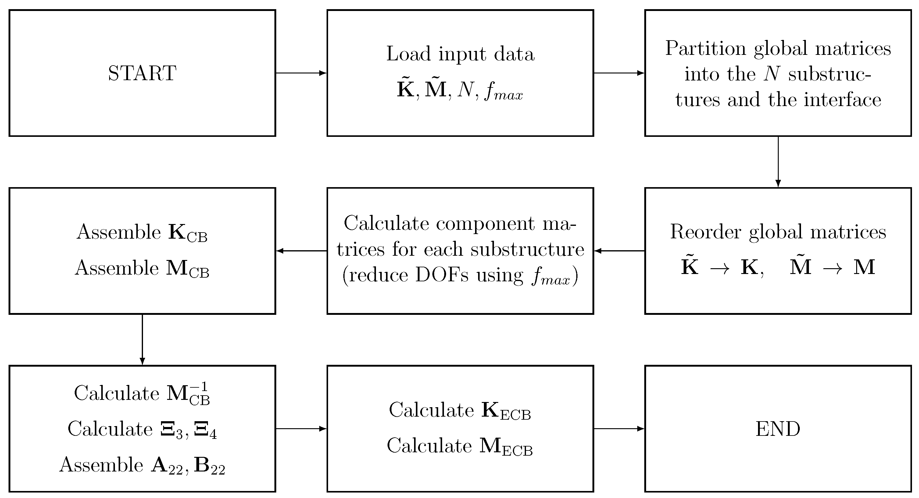
3.1. Reduction Algorithm

Computing the reduced model matrices by multiplication with the transformation matrices

$$\begin{array}{cccc}\hfill {\mathbf{K}}_{\mathrm{CB}}& ={\mathbf{T}}_0^{\mathrm{T}}\mathbf{K}{\mathbf{T}}_0,\hfill & \hfill {\mathbf{M}}_{\mathrm{CB}}& ={\mathbf{T}}_0^{\mathrm{T}}\mathbf{M}{\mathbf{T}}_0\hfill \end{array}$$

(20)

and subsequently

$$\begin{array}{cccc}\hfill {\mathbf{K}}_{\mathrm{ECB}}& ={\mathbf{T}}_1^{\mathrm{T}}\mathbf{K}{\mathbf{T}}_1,\hfill & \hfill {\mathbf{M}}_{\mathrm{ECB}}& ={\mathbf{T}}_1^{\mathrm{T}}\mathbf{M}{\mathbf{T}}_1\hfill \end{array}$$

(21)

is not efficient in case of large structures. Therefore, our reduction algorithm closely follows the derivation given in Section 2. The properties of the involved matrices are carefully examined and exploited to calculate the reduced matrices directly and efficiently.

Our reduction algorithm, outlined in Figure 1, is described in the following subsections. The original model, represented by the sparse global stiffness matrix $\tilde{\mathbf{K}}$ and sparse global mass matrix $\tilde{\mathbf{M}}$, is supplied by the user, who also chooses the number of substructures N and the cutoff frequency $f_{max}$. The global matrices are not expected to contain any prescribed (fixed) DOFs.

3.1.1. Partitioning

The original model (structure) is partitioned into N partitions (substructures) using the METIS library routines. The obtained partitions, however, cannot be readily used, because they may contain interface DOFs. Therefore, an extra post-processing step is necessary to identify the interface DOFs, remove them from the substructures, and put them into the additional $(N+1)$-th ‘interface’ partition.

Finally, the original global stiffness and mass matrix are reordered so that their rows and columns correspond to the ordering of partitions

$$\begin{array}{cccc}\hfill \mathbf{K}& =\mathbf{P}\tilde{\mathbf{K}}\mathbf{P},\hfill & \hfill \mathbf{M}& =\mathbf{P}\tilde{\mathbf{M}}\mathbf{P},\hfill \end{array}$$

(22)

where $\mathbf{P}$ represents the associated permutation matrix. Once again, it would not be efficient to form the permutation matrix explicitly and perform the double matrix multiplication. Consequently, the elements in the stiffness and mass matrices are widely distributed in the whole domain and, thus, those are inadequate for the sparse solver. To handle this issue, the matrices are reordered directly during a matrix copy operation. The reordering eliminates the need for complicated index-keeping and results in a significant simplification and speed-up of all subsequent matrix operations. The original global matrices are discarded after the reordering as they are no longer required.

3.1.2. Reduction

After the reordering, the substructural matrices ${\mathbf{K}}_s^{\left(i\right)}$, ${\mathbf{K}}_c^{\left(i\right)}$, ${\mathbf{M}}_s^{\left(i\right)}$ and ${\mathbf{M}}_c^{\left(i\right)}$ can be easily extracted for any i-th substructure, see Equations (2a)–(2c).

Each substructure $i=1,\cdots ,N$ is independent and, therefore, can be processed in parallel to obtain the following ‘substructural’ component matrices using Equations (8a)–(8d):

$$\begin{array}{c}\hfill {\mathsf{\Lambda }}_d^{\left(i\right)},\end{array}$$

(23)

$$\begin{array}{cc}\hfill {\widehat{\mathbf{D}}}_K^{\left(i\right)}& ={\left({\mathbf{K}}_c^{\left(i\right)}\right)}^{\mathrm{T}}{\mathbf{C}}^{\left(i\right)},\hfill \end{array}$$

(24)

$$\begin{array}{cc}\hfill {\widehat{\mathbf{C}}}^{\left(i\right)}& ={\left({\mathsf{\Phi }}_d^{\left(i\right)}\right)}^{\mathrm{T}}{\widehat{\mathbf{M}}}_c^{\left(i\right)},\hfill \end{array}$$

(25)

$$\begin{array}{cc}\hfill {\widehat{\mathbf{D}}}_M^{\left(i\right)}& ={\left({\mathbf{M}}_c^{\left(i\right)}\right)}^{\mathrm{T}}{\mathbf{C}}^{\left(i\right)}+{\left({\mathbf{C}}^{\left(i\right)}\right)}^{\mathrm{T}}{\widehat{\mathbf{M}}}_c^{\left(i\right)}\hfill \end{array}$$

(26)

and the following ‘interface’ component matrices using Equations (14a)–(14c):

$$\begin{array}{cc}\hfill {\widehat{\mathbf{A}}}^{\left(i\right)}& ={\left({\widehat{\mathbf{M}}}_c^{\left(i\right)}\right)}^{\mathrm{T}}{\mathbf{F}}_r^{\left(i\right)}{\widehat{\mathbf{M}}}_c^{\left(i\right)},\hfill \end{array}$$

(27)

$$\begin{array}{cc}\hfill {\widehat{\mathbf{B}}}^{\left(i\right)}& ={\left({\widehat{\mathbf{M}}}_c^{\left(i\right)}\right)}^{\mathrm{T}}{\mathbf{F}}_r^{\left(i\right)}{\mathbf{M}}_s^{\left(i\right)}{\mathbf{F}}_r^{\left(i\right)}{\widehat{\mathbf{M}}}_c^{\left(i\right)}.\hfill \end{array}$$

(28)

Although the interface component matrices will not be required until later, it is more efficient to include them here as their calculations are also independent for each substructure.

The number of reduced DOFs (i.e., dominant modes) of each substructure is determined automatically by examining the eigenvalues obtained from the eigenproblem

$${\mathbf{K}}_s^{\left(i\right)}{\mathbf{q}}^{\left(i\right)}={\mathsf{\Lambda }}_s^{\left(i\right)}{\mathbf{M}}_s^{\left(i\right)}{\mathbf{q}}^{\left(i\right)}$$

and considering only the eigenmodes that correspond to the eigenfrequencies that are lower than the user-chosen cutoff frequency $f_{max}$.

Finally, the substructural component matrices are assembled to directly obtain the reduced matrices as per Equation (9b):

$$\begin{array}{cc}\hfill {\mathbf{K}}_{\mathrm{CB}}& =\left[\begin{array}{cc}\sum {\mathsf{\Lambda }}_d^{\left(i\right)}& \mathbf{0}\\ \mathbf{0}& {\mathbf{K}}_b+\sum {\widehat{\mathbf{D}}}_K^{\left(i\right)}\end{array}\right],\hfill \end{array}$$

(29)

$$\begin{array}{cc}\hfill {\mathbf{M}}_{\mathrm{CB}}& =\left[\begin{array}{cc}{\mathbf{I}}_d& \sum {\widehat{\mathbf{C}}}^{\left(i\right)}\\ \mathrm{sym}.& {\mathbf{M}}_b+\sum {\widehat{\mathbf{D}}}_M^{\left(i\right)}\end{array}\right].\hfill \end{array}$$

(30)

3.1.3. Enhanced Reduction

To compute the enhanced reduced order matrices, we need the standard reduced order matrices and interface component matrices calculated earlier.

From the reduced model, the component matrices ${\Xi }_3$ and ${\Xi }_4$ are computed using Equation (12b):

$$\begin{array}{cc}\hfill \Xi & ={\mathbf{M}}_{\mathrm{CB}}^{-1}{\mathbf{K}}_{\mathrm{CB}}=\left[\begin{array}{cc}{\Xi }_1& {\Xi }_2\\ {\Xi }_3& {\Xi }_4\end{array}\right].\hfill \end{array}$$

(31)

However, the full matrix multiplication is not necessary, because the component matrices ${\Xi }_1$ and ${\Xi }_2$ are never used.

Independently, the component matrices ${\mathbf{A}}_{22}$ and ${\mathbf{B}}_{22}$ are assembled using Equations (14a)–(14c):

$$\begin{array}{cccc}\hfill {\mathbf{A}}_{22}& =\sum {\widehat{\mathbf{A}}}^{\left(i\right)},\hfill & \hfill {\mathbf{B}}_{22}& =\sum {\widehat{\mathbf{B}}}^{\left(i\right)}.\hfill \end{array}$$

(32)

Finally, using the component matrices, the enhanced reduced matrices are computed directly using Equations (15a) and (15b):

$$\begin{array}{cc}\hfill {\mathbf{K}}_{\mathrm{ECB}}& ={\mathbf{K}}_{\mathrm{CB}}+\left[\begin{array}{cc}{\Xi }_3^{\mathrm{T}}{\mathbf{A}}_{22}{\Xi }_3& {\Xi }_3^{\mathrm{T}}{\mathbf{A}}_{22}{\Xi }_4\\ \mathrm{sym}.& {\Xi }_4^{\mathrm{T}}{\mathbf{A}}_{22}{\Xi }_4\end{array}\right],\hfill \end{array}$$

(33)

$$\begin{array}{cc}\hfill {\mathbf{M}}_{\mathrm{ECB}}& ={\mathbf{M}}_{\mathrm{CB}}+\left[\begin{array}{cc}0& {\Xi }_3^{\mathrm{T}}{\mathbf{A}}_{22}\\ \mathrm{sym}.& {\Xi }_4^{\mathrm{T}}{\mathbf{A}}_{22}+{\mathbf{A}}_{22}{\Xi }_4\end{array}\right]+\left[\begin{array}{cc}{\Xi }_3^{\mathrm{T}}{\mathbf{B}}_{22}{\Xi }_3& {\Xi }_3^{\mathrm{T}}{\mathbf{B}}_{22}{\Xi }_4\\ \mathrm{sym}.& {\Xi }_4^{\mathrm{T}}{\mathbf{B}}_{22}{\Xi }_4\end{array}\right].\hfill \end{array}$$

(34)

Equations (33) and (34) are independent and, therefore, computed in parallel.

4. Numerical Examples

To test the parallel reduction algorithm implementation, we used several example problems. The numerical tests were carried out on the ‘Kraken’ computing cluster at the Institute of Thermomechanics ASCR, Prague, Czechia. The used cluster nodes had the following basic hardware and software configuration: 2× Intel Xeon E5-2637 v4 processor at 3.5 GHz with 16 logical cores, 256 GiB local memory, 740 GiB local SSD disk, CentOS Linux 7, and Intel Fortran compiler 18.0.2.

The following sections present the obtained results. The example problems were partitioned to different numbers of substructures. The reduction was performed on each partitioned model to test the parallel algorithm, then performed again, restricted only to one processor core to simulate a serial algorithm.

To verify the parallel algorithm, and compare the accuracy of CB and ECB methods, the relative error for the first 100 eigenvalues is also shown for both the CB reduction and the ECB reduction. The relative eigenvalue errors are considered here:

$${\xi }_i=\frac{{\overline{\lambda }}_i-{\lambda }_i}{{\lambda }_i},$$

(35)

where ${\xi }_i$ denotes the relative eigenvalue error for the i-th mode, and ${\lambda }_i$ and $\overline{{\lambda }_i}$ are the exact and approximated eigenvalues, respectively.

It should be noted that the interface size significantly impacts the computational time; therefore, if an interface reduction technique could be devised and employed, it could have a considerable effect on the computational costs.

The used processor had 16 relatively powerful cores; thus, the obtained results show about 20% to 70% difference in computational times between the serial and the parallel algorithms. We expect that the superiority of the parallel algorithm will be more apparent on a processor with a large number of less-powerful cores (64, 128, etc.).

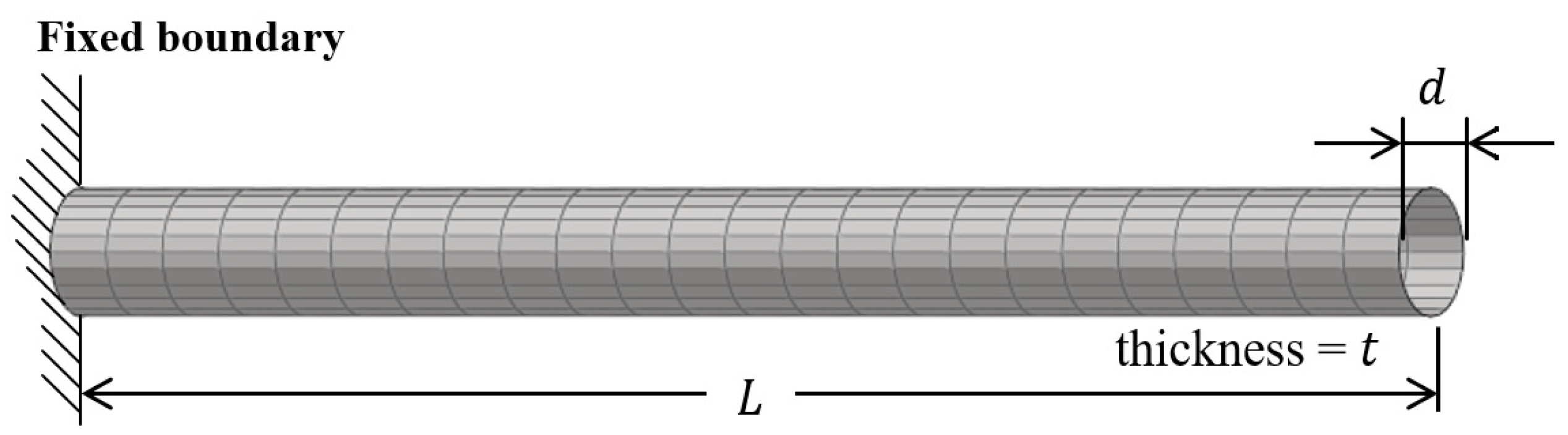
4.1. Cylindrical Shell

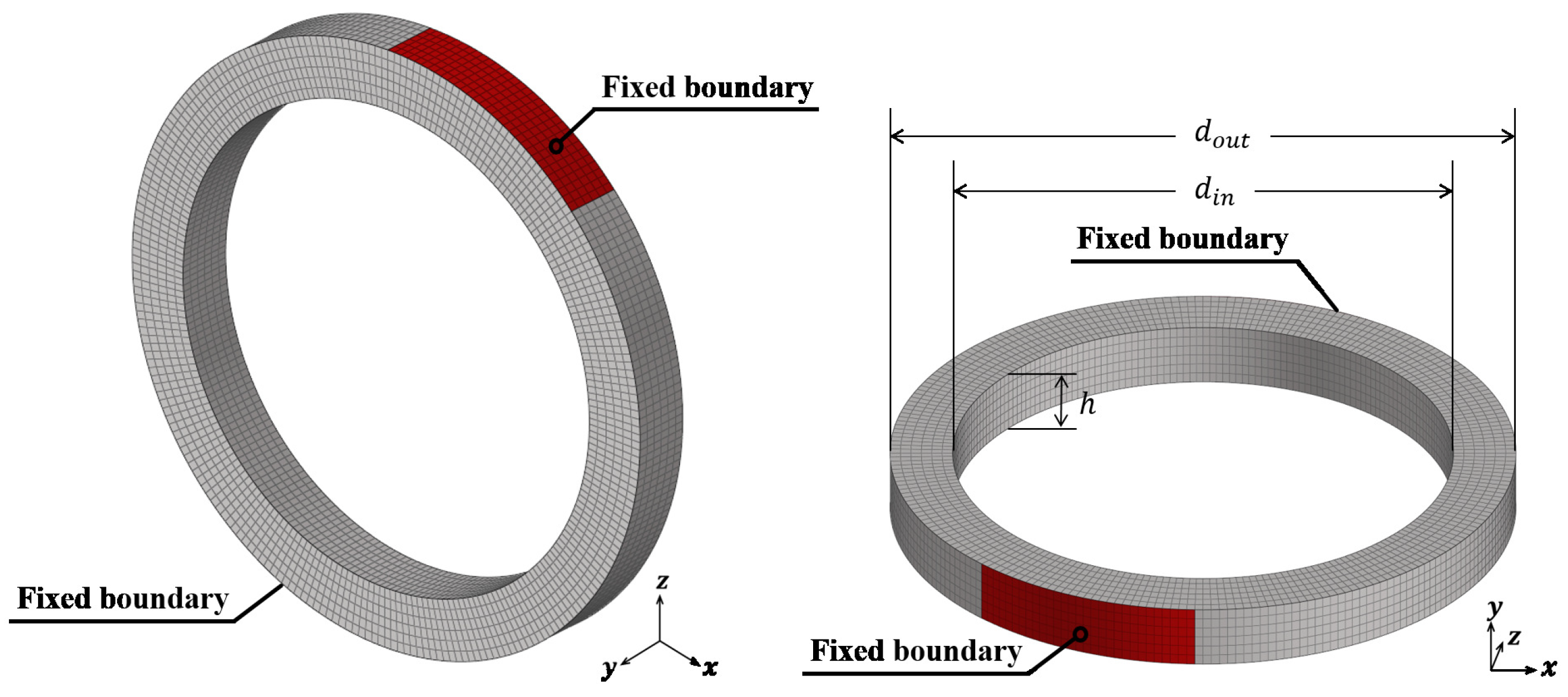
First, we implemented a cantilever cylinder problem, shown in Figure 2. The length L, thickness t, and radius d of the cantilever cylinder are 12, 0.06, and 0.5 m, respectively. Young’s modulus, Poisson’s ratio, and density are 69 GPa, 0.35, and 2700 kg/m${}^3$, respectively. The finite element model was implemented by four-node quad elements. The model had 2880 DOFs and was partitioned to 2, 4, 8, 16, and 32 substructures. The used cutoff frequency was $f_{max}=3400\mathrm{Hz}$.

To compare the accuracy for both the CB and the ECB methods, the relative error is also shown in Figure 3. The operation time at each step of the algorithm in Figure 1 is listed in

Table 1. Operation time at each step of the algorithm in the cylindrical shell problem.

Step of Algorithm	Operation Time [s]
	$\mathit{N}=\mathbf{2}$	$\mathit{N}=\mathbf{4}$	$\mathit{N}=\mathbf{8}$	$\mathit{N}=\mathbf{16}$	$\mathit{N}=\mathbf{32}$
$\mathrm{Load}\mathrm{input}\mathrm{data}$	0.2	0.2	0.2	0.2	0.2
$\mathrm{Partition}\mathrm{global}\mathrm{matrices}$	0.0	0.0	0.0	0.0	0.0
$\mathrm{Reoder}\mathrm{global}\mathrm{matrices}$	0.0	0.0	0.0	0.0	0.0
$\mathrm{Calculate}\mathrm{component}\mathrm{matrices}$	2.5	0.9	0.5	0.4	0.6
$\mathrm{Assemble}{\mathbf{M}}_{\mathrm{C}\mathrm{B}},{\mathbf{K}}_{\mathrm{C}\mathrm{B}}$	0.0	0.0	0.0	0.0	0.0
$\mathrm{Calculate}{\mathbf{M}}_{\mathrm{C}\mathrm{B}}^{-1},{\Xi }_3,{\Xi }_4,{\mathbf{A}}_{22},{\mathbf{B}}_{22}$	0.2	0.6	1.8	2.9	8.4
$\mathrm{Calculate}{\mathbf{M}}_{\mathrm{ECB}},{\mathbf{K}}_{\mathrm{ECB}}$	0.0	0.6	2.2	4.1	12.6
$\mathrm{Write}\mathrm{output}\mathrm{data}$	1.1	2.2	3.7	5.3	9.2

. The obtained reduction times listed in

Table 2. Reduction time [minute], Cylindrical Shell.

N	$min\left({\mathit{n}}_{\mathit{s}}\right)$	$max\left({\mathit{n}}_{\mathit{s}}\right)$	${\mathit{n}}_{\mathbf{int}}$	${\mathit{n}}_{\mathbf{red}}$	${\mathit{t}}_{\mathit{s}}$	${\mathit{t}}_{\mathit{p}}$
2	1320	1440	120	613	0.1	0.1
4	550	610	550	920	0.1	0.1
8	185	295	925	1195	0.2	0.1
16	60	135	1190	1397	0.3	0.2
32	10	65	1684	1795	0.6	0.5

are small and the difference between the serial and the parallel algorithm is negligible, as expected. The quantities listed in Table 2 are the number of substructures N, minimum and maximum substructure sizes $n_s$, interface size $n_{int}$, reduced model size $n_{red}$, computational time for serial reduction $t_s$, and computational time for parallel reduction $t_p$.

4.2. Solid Ring

A solid ring problem was considered with a fixed boundary condition, which is illustrated in Figure 4. The height h, the inner radii $d_{in}$, and outer radii $d_{out}$ are 0.2, 0.8, and 1.0 m, respectively. Young’s modulus, Poisson’s ratio, and density are 76 GPa, 0.3, and 2796 kg/m${}^3$, respectively. The finite element model was implemented by eight-node hexahedral elements. The model has 34,062 DOFs and was partitioned to 2, 4, 8, 16, 32, 64, and 128 substructures. The used cutoff frequency was $f_{max}=25,000\mathrm{Hz}$.

To compare the accuracy for both the CB and the ECB methods, the relative error is also shown in Figure 5. The operation time at each step of the algorithm in Figure 1 is listed in

Table 3. Operation time at each step of the algorithm in the solid ring problem.

Step of Algorithm	Operation Time [s]
	$\mathit{N}=\mathbf{2}$	$\mathit{N}=\mathbf{4}$	$\mathit{N}=\mathbf{8}$	$\mathit{N}=\mathbf{16}$	$\mathit{N}=\mathbf{32}$
$\mathrm{Load}\mathrm{input}\mathrm{data}$	1.6	1.6	1.6	1.6	1.6
$\mathrm{Partition}\mathrm{global}\mathrm{matrices}$	0.1	0.1	0.1	0.2	0.2
$\mathrm{Reoder}\mathrm{global}\mathrm{matrices}$	0.0	0.0	0.0	0.0	0.0
$\mathrm{Calculate}\mathrm{component}\mathrm{matrices}$	7148.2	1377.7	474.2	412.6	645.0
$\mathrm{Assemble}{\mathbf{M}}_{\mathrm{C}\mathrm{B}},{\mathbf{K}}_{\mathrm{C}\mathrm{B}}$	0.0	0.1	0.1	0.2	0.4
$\mathrm{Calculate}{\mathbf{M}}_{\mathrm{C}\mathrm{B}}^{-1},{\Xi }_3,{\Xi }_4,{\mathbf{A}}_{22},{\mathbf{B}}_{22}$	35.3	104.5	316.4	782.2	5299.4
$\mathrm{Calculate}{\mathbf{M}}_{\mathrm{ECB}},{\mathbf{K}}_{\mathrm{ECB}}$	3.5	22.6	234.1	1255.4	8414.1
$\mathrm{Write}\mathrm{output}\mathrm{data}$	56.8	74.9	105.8	176.8	388.3

, and the obtained results listed in

Table 4. Reduction time [minute], Solid Ring.

N	$min\left({\mathit{n}}_{\mathit{s}}\right)$	$max\left({\mathit{n}}_{\mathit{s}}\right)$	${\mathit{n}}_{\mathbf{int}}$	${\mathit{n}}_{\mathbf{red}}$	${\mathit{t}}_{\mathit{s}}$	${\mathit{t}}_{\mathit{p}}$
2	16,785	16,785	492	4696	217.1	120.8
4	8223	8247	1137	5228	86.3	26.4
8	3924	3990	2367	6240	65.0	18.9
16	1803	1962	4644	8088	82.1	43.8
32	720	883	9425	11,994	365.1	245.8
64	180	364	17,982	19,113	1698.0	1288.2
128	18	198	22,030	22,721	2989.0	2382.0

indicate that the optimal partitioning for this problem is somewhere between 5 and 15 substructures. It can be seen that a higher number of substructures increases the interface size and, subsequently, the computational time, significantly. However, a lower number of substructures, while having a smaller interface, results in large substructures, which themselves take longer to analyze and, thus, negatively affect the overall computational time.

The parallel algorithm is about 70% faster than the serial algorithm in the most favorable case tested.

4.3. Shaft Assembly

We considered a shaft problem with a free boundary condition. The shaft model consisted of five components, and the detailed features are described in Figure 6. Young’s modulus, Poisson’s ratio, and density are 210 MPa, 0.3, and 7850 kg/m${}^3$, respectively. The finite element model was implemented by four-node tetrahedral elements. The model had 64,086 DOFs and was partitioned to 2, 4, 8, 16, and 32 substructures. The used cutoff frequency was $f_{max}=100,000\mathrm{Hz}$.

Figure 7 shows the conceptual reduction process. The first one on the left is a sparse matrix modeled by the general finite element method, and a compact reduced matrix can be obtained after the reduction process.

To compare the accuracy for both the CB and the ECB methods, the relative error is also shown in Figure 8. The operation time at each step of the algorithm in Figure 1 is listed in

Table 5. Operation time at each step of the algorithm in the shaft problem.

Step of Algorithm	Operation Time [s]
	$\mathit{N}=\mathbf{2}$	$\mathit{N}=\mathbf{4}$	$\mathit{N}=\mathbf{8}$	$\mathit{N}=\mathbf{16}$	$\mathit{N}=\mathbf{32}$
$\mathrm{Load}\mathrm{input}\mathrm{data}$	3.1	3.0	3.2	3.1	3.1
$\mathrm{Partition}\mathrm{global}\mathrm{matrices}$	0.1	0.2	0.3	0.3	0.5
$\mathrm{Reoder}\mathrm{global}\mathrm{matrices}$	0.1	0.1	0.1	0.1	0.1
$\mathrm{Calculate}\mathrm{component}\mathrm{matrices}$	56,310.5	17,074.7	8282.5	6210.4	6494.7
$\mathrm{Assemble}{\mathbf{M}}_{\mathrm{C}\mathrm{B}},{\mathbf{K}}_{\mathrm{C}\mathrm{B}}$	0.1	0.2	0.4	0.9	1.5
$\mathrm{Calculate}{\mathbf{M}}_{\mathrm{C}\mathrm{B}}^{-1},{\Xi }_3,{\Xi }_4,{\mathbf{A}}_{22},{\mathbf{B}}_{22}$	174.7	1108.5	8680.3	26,534.1	61,743.2
$\mathrm{Calculate}{\mathbf{M}}_{\mathrm{ECB}},{\mathbf{K}}_{\mathrm{ECB}}$	92.8	1893.8	14,163.9	43,361.5	104,813.5
$\mathrm{Write}\mathrm{output}\mathrm{data}$	72.4	195.2	483.8	936.4	1539.2

, and the obtained results listed in

Table 6. Reduction time [minute], Shaft Assembly.

N	$min\left({\mathit{n}}_{\mathit{s}}\right)$	$max\left({\mathit{n}}_{\mathit{s}}\right)$	${\mathit{n}}_{\mathbf{int}}$	${\mathit{n}}_{\mathbf{red}}$	${\mathit{t}}_{\mathit{s}}$	${\mathit{t}}_{\mathit{p}}$
2	30,894	31,212	1980	5330	2556.3	944.2
4	14,052	15,201	5586	8573	1018.3	337.9
8	5964	7416	11,412	13,723	1204.1	526.9
16	2517	3618	16,998	18,746	2017.0	1284.1
32	1071	1677	22,912	24,186	3835.1	2909.9

indicate that the optimal partitioning for this problem is somewhere between three and seven substructures. In the most favorable case tested, the parallel algorithm is about 65% faster than the serial algorithm.

Note that the model is unconstrained, therefore, there is a gap in Figure 8 in place of the first six eigenvalues representing the free degrees of freedom.

5. Conclusions

The advanced residual modal compensation could offer dramatic accuracy improvements of the reduced matrices of the original CMS methods. However, the final reduced mass and stiffness matrices become fully populated and connected; thus, employing the parallel algorithm in the recent CMS methods with residual flexibility is difficult. To handle this issue, we introduce a component level parallel algorithm of the enhanced CB method. The reduced mass and stiffness matrices are obtained by assembling the blockwise component computation without direct transformation of the system level matrices. Automatic matrix partitioning and assembling procedures are achieved by the METIS library. Decoupling the original CB substructuring components and the ECB added matrices is essential in the proposed parallel algorithm.

The main idea of the proposed method can be extended to other iterative CMS methods with higher order residual flexibility, both primal and dual assemblies [22,32,33]. It should be noted that blockwise and decoupled formulations are prerequisites to achieve the parallel computations of iterative methods. In addition, many substructures are commonly adequate for parallel computations, but more substructures lead to larger interface DOFs in the proposed ECB formulation. Therefore, the interface reduction technique of the ECB method will be studied and considered for the high fidelity parallel ECB algorithm in the near future.

References

1. Craig, R.R.; Bampton, B.C.C. Coupling of substructures for dynamic analysis. AIAA J. 1968, 6, 1313–1319. [Google Scholar] [CrossRef] [Green Version]
2. Shabana, A.A. Dynamics of Multibody Systems; Wiley: New York, NY, USA, 1989. [Google Scholar]
3. Kim, J.G.; Han, J.B.; Lee, H.; Kim, S.S. Flexible multibody dynamics using coordinate reduction improved by dynamic correction. Multibody Syst. Dyn. 2018, 42, 411–429. [Google Scholar] [CrossRef]
4. FunctionBay, Inc. Recurdyn V9R3 User Manual; FunctionBay, Inc.: Seongnam-si, Korea, 2019. [Google Scholar]
5. Cammarata, A.; Pappalardo, C.M. On the use of component mode synthesis methods for the model reduction of flexible multibody systems within the floating frame of reference formulation. Mech. Syst. Signal Process. 2020, 142, 106745. [Google Scholar] [CrossRef]
6. Sarsri, D.; Azrar, L.; Jebbouri, A.; El Hami, A. Component mode synthesis and polynomial chaos expansions for stochastic frequency functions of large linear FE models. Comput. Struct. 2011, 89, 346–356. [Google Scholar] [CrossRef]
7. Jensen, H.A.; Millas, E.; Kusanovic, D.; Papadimitriou, C. Model-reduction techniques for Bayesian finite element model updating using dynamic response data. Comput. Methods Appl. Mech. Eng. 2014, 279, 301–324. [Google Scholar] [CrossRef]
8. Yotov, V. Stochastic Finite Element Method for Vibroacoustic Loads Prediction. Ph.D. Thesis, University of Surrey, Guildford, UK, 2020. [Google Scholar]
9. Nachtergaele, P.; Rixen, D.J.; Steenhoek, A.M. Efficient weakly coupled projection basis for the reduction of thermomechanical models. J. Comput. Appl. Math. 2010, 234, 2272–2278. [Google Scholar] [CrossRef] [Green Version]
10. Kim, S.M.; Kim, J.G.; Chae, S.W.; Park, K.C. A strongly coupled model reduction of vibro-acoustic interaction. Comput. Methods Appl. Mech. Eng. 2019, 347, 495–516. [Google Scholar] [CrossRef]
11. Wang, X.; Wang, D.; Liu, B. Efficient Acoustic Topology Optimization Using Vibro-Acoustic Coupled Craig–Bampton Mode Synthesis. Acoust. Aust. 2020, 48, 407–418. [Google Scholar] [CrossRef]
12. Kammer, D.C.; Triller, M.J. Selection of Component Modes for Craig–Bampton Substructure Representations. J. Vib. Acoust. 1996, 118, 264–270. [Google Scholar] [CrossRef]
13. Bai, Z.; Liao, B.S. Towards an Optimal Substructuring Method for Model Reduction. In PARA 2004: Applied Parallel Computing. State of the Art in Scientific Computing; Springer: New York, NY, USA, 2004; pp. 276–285. [Google Scholar]
14. Kim, S.M.; Kim, J.G.; Park, K.C.; Chae, S.W. A Component Mode Selection Method Based on a Consistent Perturbation Expansion of Interface Displacement. Comput. Methods Appl. Mech. Eng. 2018, 330, 578–597. [Google Scholar] [CrossRef]
15. Kim, S.M.; Kim, J.G.; Chae, S.W.; Park, K.C. Evaluating Mode Selection Methods for Component Mode Synthesis. AIAA J. 2016, 54, 2852–2863. [Google Scholar] [CrossRef]
16. Park, K.C.; Park, Y.H. Partitioned component mode synthesis via a flexibility approach. AIAA J. 2004, 42, 1236–1245. [Google Scholar] [CrossRef]
17. Rixen, D.J. A dual Craig–Bampton method for dynamic substructuring. J. Comput. Appl. Math. 2004, 168, 383–391. [Google Scholar] [CrossRef]
18. Kim, J.G.; Markovic, D. High-fidelity flexibility based CMS method with interface degrees of freedom reduction. AIAA J. 2016, 54, 3619–3631. [Google Scholar] [CrossRef]
19. Kim, J.G.; Lee, P.S. An enhanced Craig–Bampton method. Int. J. Numer. Methods Eng. 2015, 103, 79–93. [Google Scholar] [CrossRef]
20. Boo, S.H.; Kim, J.H.; Lee, P.S. Towards improving the enhanced Craig–Bampton method. Comput. Struct. 2018, 196, 63–75. [Google Scholar] [CrossRef]
21. Tian, W.; Weng, S.; Xia, Y.; Zhu, H.; Gao, F.; Sun, Y.; Li, J. An iterative reduced-order substructuring approach to the calculation of eigensolutions and eigensensitivities. Mech. Syst. Signal Process. 2019, 130, 361–377. [Google Scholar] [CrossRef]
22. Go, M.S.; Lim, J.H.; Kim, J.G.; Hwang, K.R. A family of Craig–Bampton methods considering residual mode compensation. Appl. Math. Comput. 2020, 369, 124822. [Google Scholar] [CrossRef]
23. Jensen, H.A.; Muñoz, A.; Papadimitriou, C.; Vergara, C. An enhanced substructure coupling technique for dynamic re-analyses: Application to simulation-based problems. Comput. Methods Appl. Mech. Eng. 2016, 307, 215–234. [Google Scholar] [CrossRef]
24. Kim, J.; Kim, J.G.; Yun, G.; Lee, P.S.; Kim, D.N. Toward modular analysis of supramolecular protein assemblies. J. Chem. Theory Comput. 2015, 11, 4260–4272. [Google Scholar] [CrossRef]
25. Krattiger, D.; Hussein, M.I. Generalized Bloch mode synthesis for accelerated calculation of elastic band structures. J. Comput. Phys. 2018, 357, 183–205. [Google Scholar] [CrossRef]
26. Kim, J.G.; Boo, S.H.; Lee, P.S. An enhanced AMLS method and its performance. Comput. Methods Appl. Mech. Eng. 2015, 287, 90–111. [Google Scholar] [CrossRef]
27. Kim, J.G.; Park, Y.J.; Lee, G.H.; Kim, D.N. A general model reduction with primal assembly in structural dynamics. Comput. Methods Appl. Mech. Eng. 2017, 324, 1–28. [Google Scholar] [CrossRef]
28. Karypis, G.; Kumar, V. A fast and highly quality multilevel scheme for partitioning irregular graphs. SIAM J. Sci. Comput. 1999, 20, 359–392. [Google Scholar] [CrossRef]
29. Wang, E.; Zhang, Q.; Shen, B.; Zhang, G.; Lu, X.; Wu, Q.; Wang, Y. Intel Math Kernel Library. In High-Performance Computing on the Intel® Xeon PhiTM; Springer: Cham, Switzerland, 2014. [Google Scholar] [CrossRef]
30. Kim, J.-G.; Seo, J.; Lim, J.H. Novel modal methods for transient analysis with a reduced order model based on enhanced Craig–Bampton formulation. Appl. Math. Comput. 2019, 344, 30–45. [Google Scholar] [CrossRef]
31. Dagum, L.; Menon, R. OpenMP: An industry standard API for shared-memory programming. Comput. Sci. Eng. 1998, 1, 46–55. [Google Scholar] [CrossRef] [Green Version]
32. Cui, J.; Xing, J.; Wang, X.; Wang, Y.; Zhu, S.; Zheng, G. A simultaneous iterative scheme for the Craig–Bampton reduction based substructuring. In Dynamics of Coupled Structures; Springer: Cham, Switzerland, 2017; Volume 4, pp. 103–114. [Google Scholar]
33. Chung, I.S.; Kim, J.G.; Chae, S.W.; Park, K.C. An iterative scheme of flexibility-based component mode synthesis with higher-order residual modal compensation. Int. J. Numer. Methods Eng. 2021, 122, 3171–3190. [Google Scholar] [CrossRef]
Figure 1. Parallel reduction algorithm.
Mathematics 09 03278 g001
Figure 2. Example mesh, Cylindrical Shell.
Mathematics 09 03278 g002
Figure 3. Comparison of reduced model accuracy, cylindrical shell. The results are obtained by (a) the CB method and (b) the ECB method, respectively.
Mathematics 09 03278 g003
Figure 4. Example mesh, Solid Ring.
Mathematics 09 03278 g004
Figure 5. Comparison of reduced model accuracy, solid ring. The results are obtained by (a) the CB method and (b) the ECB method, respectively.
Mathematics 09 03278 g005
Figure 6. Example mesh, shaft assembly.
Mathematics 09 03278 g006
Figure 7. Illustration of reduction process of the shaft assembly.
Mathematics 09 03278 g007
Figure 8. Comparison of reduced model accuracy, shaft assembly. The results are obtained by (a) the CB method and (b) the ECB method, respectively.
Mathematics 09 03278 g008