1. Introduction
The Craig–Bampton (CB) method is one of the most successful component mode synthesis (CMS) techniques [
1]. It has been implemented in various commercial software packages. The CB method was originally developed for structural vibration analysis in aerospace engineering, but it has been used in various engineering fields. The CB method is a standard coordinate reduction technique of elastic bodies (finite element model in general) in flexible multibody dynamics (FMBD) [
2,
3,
4,
5]. Recently, the CB method has been extended to structural vibration with uncertainties [
6,
7,
8], and employed to multiphysics coupled problems, such as thermomechanical models [
9] and vibro-acoustic interactions [
10,
11].
The CB method starts from substructuring (mathematically matrix partitioning). The original model is partitioned into substructures and the interface boundary. In the mode superposition manner, the substructural DOFs are presented by using few dominant modes that are substructural eigenvectors, and the constraint modes at the interface boundary are additionally employed to reassemble the substructural modes. Most eigenvectors of substructures, which are over 95% of the total DOFs in general, are neglected in the reduced matrix. It means that the accuracies of the CB-reduced matrices depend on the dominant and constraint modes. Thus, many researchers have sought to develop selection criteria of the important modes that well describe the substructural response [
12,
13,
14]. Kim et al. investigated the performance of the various mode selection methods [
15].
Conventionally, varying the numbers of retained dominant modes is one way to accuracy control of the reduced matrices. Using more modes provides better accuracy, but causes larger sizes of reduced matrices. Computational efficiency is then compromised in the desired accuracy level of the reduced matrices. The mode correction (or updating) techniques are alternatives of the mode selection methods. Considering residual flexibility to the dominant mode correction may be the most popular technique. The residual flexibility is natural in free interface CMS methods, which are the CMS methods with substructural interfaces, with classical and/or localized Lagrange multipliers [
16,
17,
18]. However, the first trial using the residual flexibility of the CB method was proposed by Kim et al. [
19], known as the enhanced CB (ECB) method. The ECB method considers the first order term of the residual flexibility in an infinite series expansion for dominant modal correction; nevertheless, it shows dramatic accuracy improvement, over (around) three or four digits, of the CB-reduced matrices, without increasing the number of the dominant modes. The ECB method has provided motives to many following works, such as iterative algorithms, considering higher order residual terms [
20,
21,
22], precise stochastic model reduction [
23], multiscale model reduction [
24,
25], eigenvalue problem solvers [
26], etc. Kim et al. [
27] generalized the model reduction with the residual flexibility, and summarized the relationship between the CMS and dynamic condensation methods. The accuracy improvement of the ECB families is clear, but treatments of the residual flexibility for the modal correction require additional computational costs. In particular, the ill-conditioned problems are severe through the higher iteration steps. Regularization may be considered to handle this problem. Go et al. [
22] proposed a high fidelity iterative ECB method within a standard 16 digit computation, and compared the results with the other iterative techniques required over 32 digits to get stable numerical solutions. However, effective computation has been less investigated and, thus, the ECB family has been limited when applied into large-scale structural problems.
To overcome this issue, an efficient parallelization of the ECB method is presented. The original ECB formulation is then reorganized first for the parallel computation. In this numerical algorithm, the METIS library [
28] is used to partition the structure automatically, then the reduced matrices are calculated directly by assembling blockwise contributions from substructures, exploiting the fact that substructures are independent and can be processed in parallel. The Intel MKL library [
29] provides the necessary matrix operations. The blockwise ECB formulation for the applicability of the parallel computation is presented in
Section 2. The details of the parallel implementation of the ECB method, including the algorithm, are described in
Section 3. The performances of both accuracy and computational efficiency of the proposed algorithm are investigated in
Section 4. Conclusions are presented in
Section 5.
2. The Enhanced Craig–Bampton Method
The enhanced Craig–Bampton method [
19] is presented in this section. In the substructuring manner, the original formulations are explicitly presented and modified for parallel implementation. The equations of the motion of structural dynamics can be written as
where
and
are mass and stiffness matrices, respectively;
and
are displacement and force vectors, respectively. The subscripts
s,
b, and
c denote substructure, interface boundary, and coupling matrices (or vectors), respectively. Here, the matrices and vectors with respect to substructures are
where
and
are block diagonal mass and stiffness matrices of substructures, respectively.
denotes number of substructures.
In the CB method [
1], the original displacement vector
is approximated by combining the substructural eigenvectors and interface constraint modes as follows:
where an overbar denotes an approximation.
is a transformation matrix,
is a generalized coordinate vector of substructures,
is a constraint matrix, and
is an identity matrix of interface boundary, respectively.
is a substructural eigenvector matrix calculated from the following eigenvalue problems:
where
is the number of DOFs of the
kth substructure. The number of total DOFs is defined as
(
), in which
is the number of interface boundary DOFs. The
ith eigenvalue and its corresponding eigenvector of the
kth substructure are denoted as
and
, respectively. Then, the component matrices and vectors of Equation (
3) are
Note that the eigenvectors in this paper are defined as mass-orthonormal vectors.
By decomposing dominant and residual eigenvectors, the approximated displacement vector in Equation (
3) can be rewritten as
where
and
are dominant and residual substructural eigenvector matrices, respectively, and both are block diagonal matrices.
and
are the corresponding generalized coordinate vectors, respectively. The subscripts
d and
r denote the dominant and residual terms, respectively. Here,
and
denote numbers of the dominant and residual modes, which are defined as
and
, respectively. The number of the dominant modes is much less than the number of the residual modes in general structural vibration (
).
Using Equations (6a)–(6d) in Equations (1a)–(1c), we obtain the equations of motion for the partitioned structure
and the component matrices are
From the mass-orthonormal condition,
and
are identity matrices, and
and
are diagonal matrices with the dominant and residual eigenvalues computed from Equation (
4), respectively.
The following reduced eigenvalue problem of the original CB method can be obtained by neglecting the terms of the generalized coordinates with respect to the residual modes from Equations (7a) and (7b):
in which
is an angular frequency (
). This is also derived by using the CB transformation matrix
from
, neglecting the residual modes (
) in Equations (6a)–(6d) as
Equation (
10) means that the residual mode are simply neglected in the original CB method, but considering the residual mode effect in the model reduction process provides a change to dramatic improvement. It is a main idea of the enhanced CB method. From the second row of Equations (7a) and (7b), assuming
, the generalized coordinate vector of the residual modes,
, can be expressed as
Using Equation (
11) in Equations (7a) and (7b),
and
are redefined, and then the displacement vector in Equations (6a)–(6d) is modified as
where
is the residual flexibility of the
kth substructure, which is simply computed by its full and dominant flexibilities.
defined by using the CB-reduced matrices is an asymmetric matrix. The new transformation matrix
can be obtained by the original CB transformation matrix
and the additional transformation matrix
, including the residual modal effect. The derivation details are well presented in Reference [
19].
Using the enhanced transformation matrix
in Equation (
10) instead of
, the following enhanced reduced mass and stiffness matrices are defined
It clearly shows that the residual mode correction is additionally considered in the ECB-reduced matrices. Therefore, the ECB formulation provides more accurate reduced matrices than the original CB method.
Using the orthogonal condition and investigating the component matrix level in Equations (13a) and (13b), we obtain
Using Equations (14a)–(14c), the reduced matrices in Equations (13a) and (13b) are rewritten as
and then its eigenvalue problem is
It clearly shows that the sizes of the ECB-reduced matrices are exactly the same as the sizes of the CB-reduced matrices.
After solving Equation (
16), the original displacement vector can be obtained by back-transformation from the reduced unknown vector as
This is known as the
modal-displacement method [
30], which is a standard domain recovery technique. It also clearly shows that the substructural displacement vector
is only approximated and needs to recover.
Considering Equations (12a)–(12d), the ECB transformation matrix is explicitly written as
and
is then computed by
4. Numerical Examples
To test the parallel reduction algorithm implementation, we used several example problems. The numerical tests were carried out on the ‘Kraken’ computing cluster at the Institute of Thermomechanics ASCR, Prague, Czechia. The used cluster nodes had the following basic hardware and software configuration: 2× Intel Xeon E5-2637 v4 processor at 3.5 GHz with 16 logical cores, 256 GiB local memory, 740 GiB local SSD disk, CentOS Linux 7, and Intel Fortran compiler 18.0.2.
The following sections present the obtained results. The example problems were partitioned to different numbers of substructures. The reduction was performed on each partitioned model to test the parallel algorithm, then performed again, restricted only to one processor core to simulate a serial algorithm.
To verify the parallel algorithm, and compare the accuracy of CB and ECB methods, the relative error for the first 100 eigenvalues is also shown for both the CB reduction and the ECB reduction. The relative eigenvalue errors are considered here:
where
denotes the relative eigenvalue error for the
i-th mode, and
and
are the exact and approximated eigenvalues, respectively.
It should be noted that the interface size significantly impacts the computational time; therefore, if an interface reduction technique could be devised and employed, it could have a considerable effect on the computational costs.
The used processor had 16 relatively powerful cores; thus, the obtained results show about 20% to 70% difference in computational times between the serial and the parallel algorithms. We expect that the superiority of the parallel algorithm will be more apparent on a processor with a large number of less-powerful cores (64, 128, etc.).
4.1. Cylindrical Shell
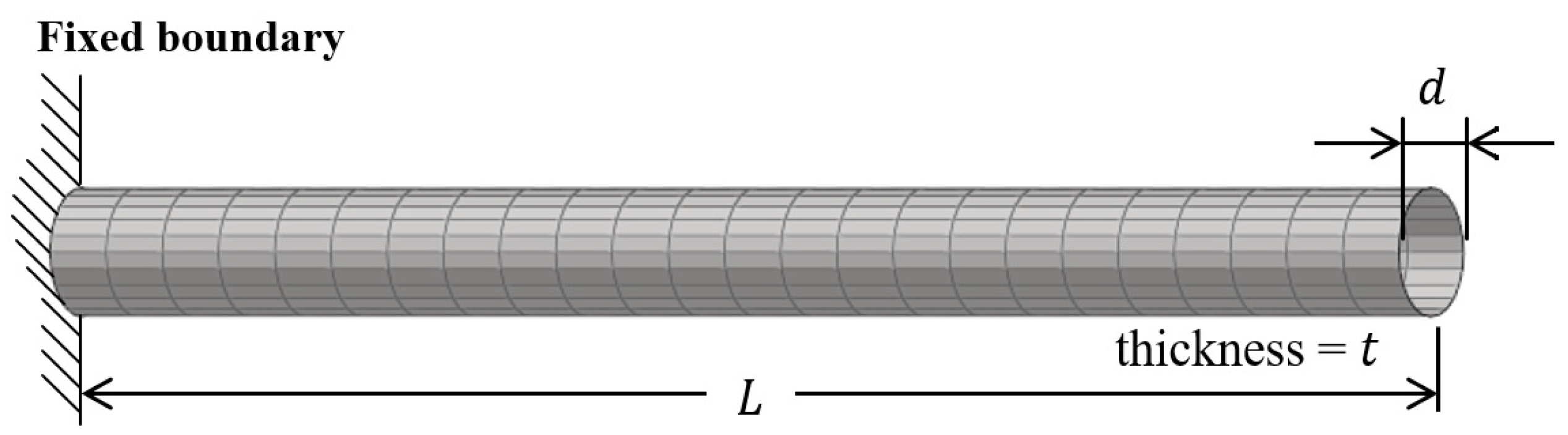
First, we implemented a cantilever cylinder problem, shown in
Figure 2. The length
L, thickness
t, and radius
d of the cantilever cylinder are 12, 0.06, and 0.5 m, respectively. Young’s modulus, Poisson’s ratio, and density are 69 GPa, 0.35, and 2700 kg/m
, respectively. The finite element model was implemented by four-node quad elements. The model had 2880 DOFs and was partitioned to 2, 4, 8, 16, and 32 substructures. The used cutoff frequency was
.
To compare the accuracy for both the CB and the ECB methods, the relative error is also shown in
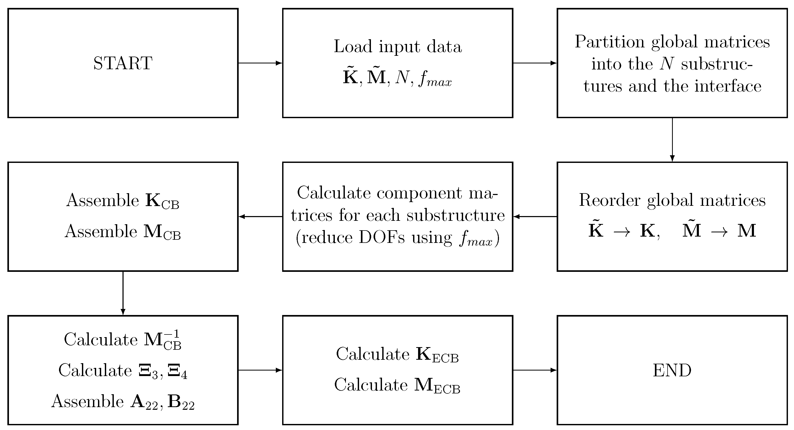
Figure 3. The operation time at each step of the algorithm in
Figure 1 is listed in
Table 1. The obtained reduction times listed in
Table 2 are small and the difference between the serial and the parallel algorithm is negligible, as expected. The quantities listed in
Table 2 are the number of substructures
N, minimum and maximum substructure sizes
, interface size
, reduced model size
, computational time for serial reduction
, and computational time for parallel reduction
.
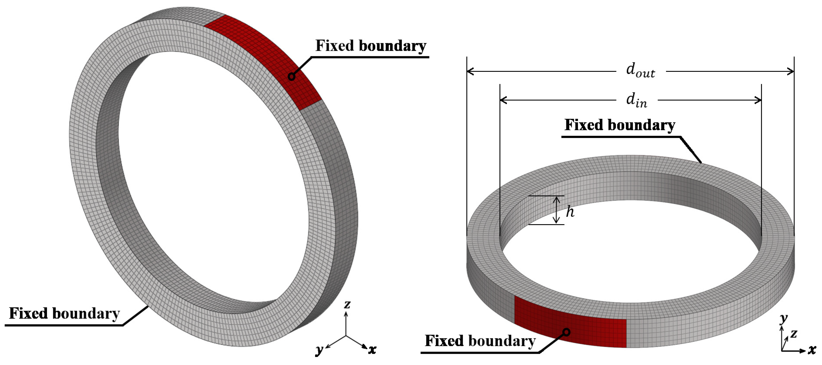
4.2. Solid Ring
A solid ring problem was considered with a fixed boundary condition, which is illustrated in
Figure 4. The height
h, the inner radii
, and outer radii
are 0.2, 0.8, and 1.0 m, respectively. Young’s modulus, Poisson’s ratio, and density are 76 GPa, 0.3, and 2796 kg/m
, respectively. The finite element model was implemented by eight-node hexahedral elements. The model has 34,062 DOFs and was partitioned to 2, 4, 8, 16, 32, 64, and 128 substructures. The used cutoff frequency was
.
To compare the accuracy for both the CB and the ECB methods, the relative error is also shown in
Figure 5. The operation time at each step of the algorithm in
Figure 1 is listed in
Table 3, and the obtained results listed in
Table 4 indicate that the optimal partitioning for this problem is somewhere between 5 and 15 substructures. It can be seen that a higher number of substructures increases the interface size and, subsequently, the computational time, significantly. However, a lower number of substructures, while having a smaller interface, results in large substructures, which themselves take longer to analyze and, thus, negatively affect the overall computational time.
The parallel algorithm is about 70% faster than the serial algorithm in the most favorable case tested.
4.3. Shaft Assembly
We considered a shaft problem with a free boundary condition. The shaft model consisted of five components, and the detailed features are described in
Figure 6. Young’s modulus, Poisson’s ratio, and density are 210 MPa, 0.3, and 7850 kg/m
, respectively. The finite element model was implemented by four-node tetrahedral elements. The model had 64,086 DOFs and was partitioned to 2, 4, 8, 16, and 32 substructures. The used cutoff frequency was
.
Figure 7 shows the conceptual reduction process. The first one on the left is a sparse matrix modeled by the general finite element method, and a compact reduced matrix can be obtained after the reduction process.
To compare the accuracy for both the CB and the ECB methods, the relative error is also shown in
Figure 8. The operation time at each step of the algorithm in
Figure 1 is listed in
Table 5, and the obtained results listed in
Table 6 indicate that the optimal partitioning for this problem is somewhere between three and seven substructures. In the most favorable case tested, the parallel algorithm is about 65% faster than the serial algorithm.
Note that the model is unconstrained, therefore, there is a gap in
Figure 8 in place of the first six eigenvalues representing the free degrees of freedom.


