Abstract
The stream sediment (SS) records evolution information of the water system structure and sedimentary environment in specific regions during different geological periods, which is of great significance for studying the ancient planetary environment and the law of water system changes. Based on the SS of different geographical environments on Earth, remote laser-induced breakdown spectroscopy (remote-LIBS) technology combined with the multidimensional scaling-back propagation neural network (MDS-BPNN) algorithm was used to conduct an in-depth analysis of remote qualitative and quantitative detection of the elemental composition and content of SS. The results show that the detection system based on remote LIBS combined with an artificial neural network algorithm can achieve an ideal quantitative analysis of major and trace elements. The coefficients of determination (R2) of the test set for major elements is greater than 0.9996, and the root mean square error (RMSE) is less than 0.7325. The coefficients of determination (R2) of the test set for trace elements is greater than 0.9837, and the root mean square error is less than 42.21. In addition, for the application scenario of exploring extraterrestrial life, biominerals represented by stromatolite phosphorite (SP) are easy to form sand and enter into SS under weathering. Therefore, this paper discusses the feasibility of using remote-LIBS technology to detect and identify such minerals under the disappearance of SPs’ macro- and micro-characteristics. From our research, we can find that remote-LIBS technology is the preferred candidate for discovering dust-covered biominerals. In geological environments rich in water system sedimentary rocks, such as Mars’ ancient riverbeds, LIBS technology is crucial for deciphering the “life signals” hidden in the Martian sand.
1. Introduction
Stream sediment (SS) plays an essential role in exploring earth minerals. By studying the distribution of elements in SSs, we can find geochemical anomalies, delineate prospecting prospects and favorable metallogenic areas, and provide the basis for further detailed geochemical exploration and geological survey. More importantly, quantitative analysis of major, minor, and trace elements in SS can be used to reconstruct paleoclimate, paleosalinity, and paleo-redox environments [1]. In addition, geochemical investigations of major, minor, and trace elements from bedload sediments can link the fluvial with the marine depositional system [2]. SS can also be used for potential risk assessment of the ecological environment by measuring the potential ecological risk index of heavy metals and analyzing the main factors that cause heterogeneity in the potential environmental risk index. X-ray fluorescence spectroscopy (XRF), inductively coupled plasma emission mass spectroscopy (ICP-MS), inductively coupled plasma optical emission spectroscopy (ICP-OES), atomic absorption spectroscopy (AA), and micro scanning X-ray diffusion (SXRD) are still the primary technical means for analyzing river sediment at present [2,3,4,5]. However, to achieve good measurement accuracy, on-site sampling and laboratory nuanced analysis strategies are still the main factors, which restrict the realization of large-scale, high-efficiency, and low-cost in situ remote detection of SS. Therefore, achieving a remote, in situ, and efficient qualitative and quantitative detection method for major, minor, and trace elements in SS is a research hotspot, especially for applying deep space exploration. Laser-induced breakdown spectroscopy (LIBS) is plasma emission spectroscopy formed by a high-energy pulsed laser focusing on the surface of a sample and creating spectroscopy composed of atoms and ions excited by electrons by ablating the material [6,7]. LIBS is an atomic spectroscopy comprising “unique fingerprints” generated by different elements, which can almost achieve almost all periodic table elements. The most valuable feature of LIBS is its strong signal and high detection efficiency, which can meet the detection needs of various functions such as remote in situ and short-range microscopy [8,9,10,11].
LIBS is a technique that can be used for stand-off analysis of soils at reduced air pressures and in a simulated Martian atmosphere. This technique has been shown to be feasible for space exploration [12,13,14,15] and geoscience [16,17,18,19]. Under specific physical and chemical conditions, LIBS can also obtain molecular emission spectra. For the first time, researchers conducted LIBS detection of organic compounds of interest in astrobiology in the Mars simulated atmosphere. In addition, they studied the impact of the Mars atmosphere on the new combination mechanism of laser-induced plasma of organic compounds of interest in astrobiology [20]. In addition, the team also conducted research on the remote-LIBS in situ rapid identification of stromatolite phosphorite (SP) that preserve early life on Earth, targeting the application scenarios of extraterrestrial life detection [10]. The research of geochemistry and astrobiology is mainly focused on detecting and identifying biological molecules with a reference value for discovering Martian life. The study of biomarkers of Martian-like landforms on the Earth, or “traces” left by early life on the Earth, can help us to find life on the red planet or its “traces” [21,22]. Life’s evolution process on Earth cannot be separated from the participation of water, so the types of planetary (such as Mars) landforms related to water are the Important geological environment for deep space in situ exploration [23].
The main types of water-related landforms are ancient lakes, rivers, and deltas, and these unique landforms have a high spatial correlation with the distribution of water-bearing minerals. Primitive life is highly likely to occur in such areas, and its “traces” of life can be preserved in some way [24]. Therefore, remote in situ detection of major and trace elements in SSs in sedimentary environments such as lakes, rivers, or deltas is of great reference value for searching for extraterrestrial life. At variance with most scenario’s on Earth SS on Mars are expected to be dried for sure. Stromatolites are layered biochemical accretion structures formed by early life on Earth and are the sedimentary structures that preserve the oldest life on Earth. The growth environment of stromatolites is closely related to water-related geomorphic types, and stromatolites have also become indicative minerals for searching for extraterrestrial life [24,25].
Referring to the planetary scale stromatolite sedimentary structure formed by the large-scale accumulation of Precambrian microorganisms on the Earth, during a long period of warm and humid climate, Mars may also have a biological sedimentary structure similar to that created by the direct or indirect influence of organisms on the Earth. Even if this biological sedimentary structure does not reach the planetary scale, it appears in the form of small-scale and scattered distribution. But this assumption is also sufficient to drive human research on identifying and detecting stromatolites in different geological backgrounds. In an extreme space environment, weathering will drive the dusting of this kind of biominerals. Finding and quantifying this kind of biominerals is a vital work to look for the “relics” of Martian life in the future.
In this study, for the first time, a laboratory simulation analysis study was conducted to identify and quantify the SPs powder in SS. SPs powder no longer possesses macroscopic and microscopic morphological characteristics, making it difficult to evaluate them effectively through microscopic images or Raman mapping. This study first identifies and quantifies the main and trace elements in SS to verify the potential application of remote-LIBS in quantifying the elemental content of SS. Second, machine learning algorithms are used to achieve dimensionality reduction clustering of high-dimensional data, analyze the recognition problem of SPs, and evaluate their detection limits in SSs. Finally, the concentration of SPs was quantified using neural network algorithms. By introducing the molecular emission spectrum (molecular laser-induced fluorescence, MLIF), the feasibility of using LIBS to discover biominerals powder in SS has been confirmed. The remote application proposed is from the Mars Rover arm, already designed and realized with a LIBS probe operating at 7 m distance. Therefore, this study is a fundamental study aimed at further analyzing the measured LIBS data on Mars.
2. Materials and Methods
2.1. Sample Description and Preparation
The article used 28 certified reference materials (CRMs) and 1 typical stromatolite phosphate rock (SP). The content of CRMs is shown in Table 1, including 16 chemical compositions of stream sediments (CCSSs), 4 chemical compositions of floodplain sediments (CCFSs), and 8 chemical compositions of soils (CCSs). The preparation process for the collected CCSSs, CCFSs, and CCSs samples is as follows: after drying, impurity removal, coarse crushing, passing through a 1 mm sieve, and drying at a temperature above 100 °C for 24 h, removing water, inactivating, and grinding with a high alumina ceramic ball mill until the particle size is less than 80 μm (accounting for more than 99%). The geographical and climatic characteristics of the sampling area are diverse, with temperature zones covering the temperate, warm temperate, subtropical, tropical, and Qinghai Tibet Plateau regions. The climatic characteristics of the sampling area include temperate monsoon climate, temperate continental climate, subtropical monsoon climate, tropical monsoon climate, and plateau mountain climate. The dry and wet characteristics of the sampling area include humid, semi-humid, arid, and semi-arid regions, as shown in Figure 1a. Using the SS of the Yangtze River in Wuhan as the geological background, 21 types of mineral mixed powders (MMPs) were prepared by mixing SP powder with CRM (GBW07309) in the proportion shown in Table 2. The research team purchased all CRMs mentioned in the paper from Weiye Metrology and Technology Research Group Co., Ltd., Beijing, China (http://www.bzwz.com) (accessed on 23 May 2023). Readers can obtain all detailed information of CRMs by searching for the reference IDs.

Table 1.
The abundance of the major, minor, and trace elements (wt.%) and its geographical location of the 28 CRMs.
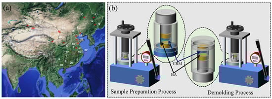
Figure 1.
Geographical location of sampling area and preparation process of CRMs experimental target: (a) geographical location of sampling area; (b) preparation process of CRMs experimental target.
Table 2.
The abundance of the major and trace elements (wt.%) of the 21 MMPs.
The preparation of experimental targets mainly includes the sample preparation and demolding processes; the detailed process is shown in Figure 1b. It should be emphasized that the sample preparation process involves laying a layer of boric acid powder first, followed by a layer of CRM powder. Boric acid is prone to molding under strong pressure, so in this study, boric acid was selected as the substrate for CRM. The pressure exerted by the tablet press on the sample is 250 MPa (lasting 5 min).
2.2. Experimental Device
The experimental setup built by the team is shown in Figure 2. The system can be divided into four parts: signal excitation (collection) system, signal acquisition system, digital delay control system, and sample movement platform. The signal excitation (collection) system mainly comprises the pulse laser, the improved Cassegrain optical system, the smit mirror, and other main components. The system is primarily responsible for using the pulse laser to generate plasma emission and collecting the generated LIBS signal; The signal acquisition system is mainly composed of Avantes multi-channel spectrometer, which is primarily responsible for collecting spectral signals covering deep ultraviolet to near-infrared using multiple portable spectrometers. The digital delay control system is composed mainly of a pulse delay generator DG645, which is primarily responsible for using the synchronous delay to control the signal acquisition time sequence of the laser and spectrometer, and achieve accurate pickup of single pulse signals. The sample moving platform is mainly composed of a rotating platform and a vacuum chamber, primarily responsible for using the rotating platform to replace experimental targets automatically. In addition, the vacuum chamber can simulate simulated environmental experiments with different atmospheres and pressures. It should be noted that this study only simulated the atmospheric pressure of Mars in the vacuum chamber and did not fill it with the simulated Martian atmosphere. The pulsed laser is an Nd: YAG Q-switched laser (Lapa-80, Beamtech Optronics Co., Ltd., Beijing, China), with a laser wavelength of 1064 nm, a pulse width of 8 ns, a maximum pulse energy of 80 mJ, and a maximum repetition frequency of 20 Hz. 8-channel spectrometer (AVS-RACKMOUNT-USB2, AvaSpec Multi-Channel Spectrometer, Avantes Co., Ltd., Apeldoorn, The Netherlands) with a slit of 10 μm for each channel. The spectral acquisition ranges of the eight channels are 200~320, 318~420, 417~505, 500~565, 565~670, 668~750, 745~930, and 920~1070 nm. The spectral resolution of the first channel to the fourth channel is 0.09 to 0.13 nm, the spectral resolution of the fifth and sixth channels is 0.1 to 0.18 nm, and the spectral resolution of the seventh and eighth channels is 0.2 to 0.28 nm. The exposure time of a single LIBS is 1 ms, and a single LIBS corresponds to a signal generated by one laser pulse. The distance between the experimental target and the device is 7 m, and the time collected by the spectrometer is 159 microseconds and 898 nanoseconds later than the laser trigger time. At a working distance of 7 m, the focal spot diameter of the pulsed laser on the sample surface is less than 200 μm.
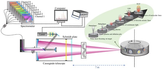
Figure 2.
Structural diagram of sample and experimental system.
As shown in Figure 2, the process of plasma emission generated by the contact between a pulse laser and the sample target material includes a pulse laser focusing on the target, small plasma, and insertion dots, forming plasma, emission of continuous light, and emission of discrete atomic lines. Therefore, the digital delay control system selects the period of emission of atomic and molecule lines by adjusting the time sequence of the laser and spectrometer.
2.3. Spectral Data Preprocessing
The preprocessing of spectral data mainly includes baseline correction, noise reduction, redundant data deletion, mean normalization, multi-channel stitching, and other steps. Baseline correction is essential in removing the influence of the instrument’s dark current, background noise interference, and continuous light. Through baseline correction, more pure LIBS signals can be extracted. Noise reduction is the process of reducing noise in spectral signals, further highlighting the inherent characteristics of LIBS signals. Redundant data deletion refers to the removal of spectral segments without signal response, achieving the effect of reducing data dimensionality by deleting useless data. Normalization is an essential means to reduce the impact of factors such as laser energy jitter, defocusing, and different detection distances on LIBS data. Multi-channel stitching is the best scheme to realize LIBS spectral coverage from deep ultraviolet to near-infrared high spectral resolution detection. Figure 3 shows some core processes of spectral data preprocessing implemented, including baseline correction, noise removal, redundant data deletion, and mean normalization. It is worth emphasizing that the data processing of each channel above is conducted separately and without interference with each other. This article uses baseline estimation and denoising using sparsity (BEADS) algorithm in the baseline correction and noise reduction process. Some parameters of the BEADS algorithm require human intervention to achieve the optimal processing effect through regulation [26,27]. The three essential core parameters are distinguished as off frequency (fc), filter order parameter (d), and geometry parameter (r), where fc is 0.01, d is 1.0, and r is 6.
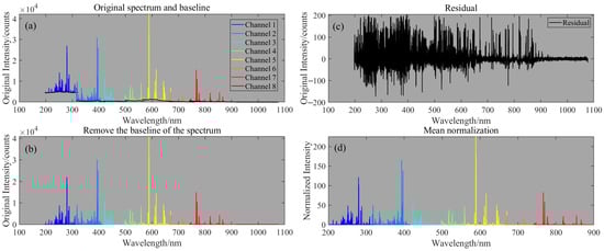
Figure 3.
LIBS baseline correction and noise reduction: (a) original spectrum and baseline; (b) remove the baseline of LIBS; (c) residual; (d) mean normalization.
2.4. Building Quantitative Analysis Models
In terms of data processing, Matlab R2020a (Massachusetts Institute of Technology, Natick, MA, USA) is used for data analysis and scientific drawing, respectively. This study detected 28 types of CRMs targets, each of which collected 30 LIBS spectra, forming 840 spectral datasets. The training set, validation set, and test set were randomly generated in a ratio of 14:3:3. Construct a quantitative analysis model for major, minor, and trace elements based on the dataset, where major element oxides include SiO2, Al2O3, TFe2O3, TiO2, CaO, MgO, K2O, and Na2O, and other elements include Ba, Be, Li, Rb, and Sr.
The original high-dimensional data contains a large amount of redundant information, which can introduce errors in practical applications and affect the results of qualitative and quantitative analysis. By reducing the dimensionality of the data and extracting feature values, useful information can be picked up, and useless information can be eliminated, making it easier to calculate and visualize. The two commonly used dimensionality reduction methods are principal component analysis (PCA) [28] and multidimensional scaling (MDS) [29]. The most significant difference between MDS and PCA is that MDS focuses on the internal features of high-dimensional data rather than preserving the maximum separability of the data. As a result, MDS can maintain the relative relationship of high-dimensional data in the original space without requiring prior knowledge and simple calculation, resulting in better visualization results. The back propagation neural network (BPNN) is a classic neural network structure composed of three layers: the input layer, the hidden layer, and the output layer. The hidden layer transmits essential information between the input and output layers. When faced with complex problems, BPNN can be composed of multiple hidden layers to form a deep learning network, which can realize the fitting of multi-input and multi-output arbitrary nonlinear functions through the nesting of multiple functions [30,31,32]. Figure 4a,b show single-neuron mathematical models and BPNN neural network structures.
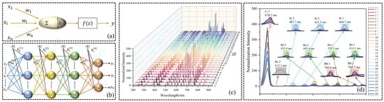
Figure 4.
Neural network structure and LIBS spectra: (a) neuron model; (b) structure of BPNN; (c) LIBS spectra of 28 CRMs; (d) splicing of LIBS spectral peaks of minor and trace elements.
Figure 4c shows the LIBS spectra of 28 CRMs. The major elements contribute most of the characteristic information of the target LIBS spectrum. Therefore, for the quantitative analysis of the major elements, the MDS dimensionality reduction method of the full spectrum is adopted, that is, while removing the redundant information, extracting the characteristic values, and retaining the relative relationship of the high latitude data. Then, BPNN quantitative analysis model is constructed. The spectral lines of minor and trace elements such as Ba, Be, Li, Rb, and Sr are relatively simple and account for a small proportion of the spectrum of the whole spectrum. Therefore, first, the characteristic spectral peaks of these elements are selected by human intervention (Figure 4d), and all spectral peaks are spliced for MDS dimensionality reduction processing. Then, the BPNN quantitative analysis model is constructed by the low latitude data after dimensionality reduction.
3. Results
3.1. LIBS Spectra of CRMs and Its MDS Dimensionality Reduction Visualization
Each CRM has 30 spectra, so we can obtain 840 preprocessed spectral data and characteristic peak splicing curves for the quantitative analysis of major and other elements, respectively. We will perform MDS dimensionality reduction on these data and select the first three dimensions of data to present the clustering features of the dimensionality reduction data, as shown in Figure 5. Figure 5a–c show the MDS dimensionality reduced 3D visualization of LIBS spectral data for 28 CRMs from different angles. Figure 5d–f show the MDS dimensionality reduced 3D visualization of LIBS peak splicing curves for minor and trace elements of 28 CRMs from different angles. The experimental results in Figure 5 indicate that regardless of the full LIBS spectrum and feature peak splicing curve dataset, the dimensionality reduction data of each type of CRMs has good clustering performance, and there are significant differences among different CRMs. This clustering effect benefits from MDS projecting high-dimensional data into a low-dimensional space, making similar objects in the high-dimensional space closer together in the low-dimensional space. The dimensionality reduction data provides a basis for qualitative analysis of mineral categories and quantitative analysis of major and other elements in minerals.
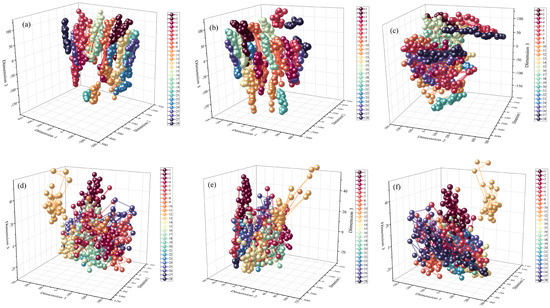
Figure 5.
The 3D Visualization of MDS dimensionality reduction: (a–c) 3D visualization of full spectrum data dimensionality reduction; (d–f) 3D visualization of characteristic peaks/bands dimensionality reduction.
3.2. Quantitative Analysis of Major Element Oxides
The structure of the quantitative analysis model of the BPNN consists of four hidden layers, and the number of neurons in each layer is 35, 15, 12, 10. The activation function uses the sigmoid function, with a learning rate of 0.01, a maximum training number of 100, and a minimum error of 0.05. We divide the training set, validation set, and test set into a ratio of 14:3:3 and construct a BPNN quantitative analysis model. In the training process of the BPNN quantitative analysis model, dimensionality reduction data of the entire spectrum is used as the model input, and the content of eight major element oxides is used as the model output. The overall prediction performance of the eight main element quantitative analysis models is shown in Figure 6. Figure 6a shows the quantitative analysis effect of the major element oxides in the LIBS spectral training sets of CRMs, Figure 6b shows the quantitative analysis effect of the major element oxides in the LIBS spectral validation sets of CRMs, and Figure 6c shows the quantitative analysis effect of the major element oxides in the LIBS spectral testing sets of CRMs.
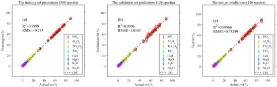
Figure 6.
Quantitative prediction of major element oxides based on MDS-BPNN model: (a) quantification effect of major element oxides in the training set; (b) quantification effect of major element oxides in the validation set; (c) quantification effect of major element oxides in the test set.
To further compare the predictive effects of BPNN quantitative analysis on eight major element oxides, the prediction results of the test set were analyzed separately by different element, as shown in Figure 7 and Figure 8. The results showed that except for TiO2 and K2O. The coefficients of determination (R2) of the quantitative analysis results for the other six major element oxides were all greater than 0.9671, and the root mean square error (RMSE) was less than 0.75. The quantitative analysis results of TiO2 and K2O have R2 values of 0.755 and 0.895, respectively, and RMSE values of 0.20 and 0.31, respectively. The content of TiO2 and K2O in 28 types of CRMs is relatively low, resulting in insignificant characteristics in LIBS spectra. In high-dimensional data compression, the extracted features of these two elements are not apparent, so the predictive effect of BPNN quantitative analysis on these two elements is average.
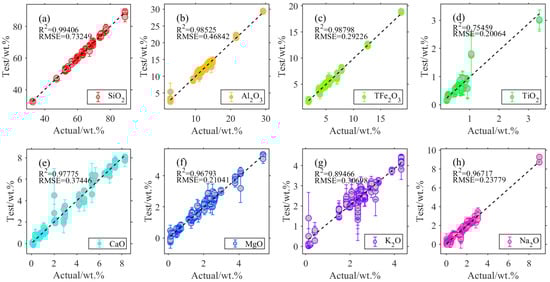
Figure 7.
Quantitative prediction of eight major element oxides in the test set based on MDS-BPNN model: (a) quantification effect of SiO2; (b) quantification effect of Al2O3; (c) quantification effect of TFe2O3; (d) quantification effect of TiO2; (e) quantification effect of CaO; (f) quantification effect of MgO; (g) quantification effect of K2O; (h) quantification effect of Na2O.
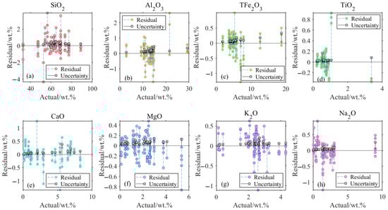
Figure 8.
Residual and uncertainty of eight major element oxides in the test set based on MDS-BPNN model: (a) residual and uncertainty of SiO2; (b) residual and uncertainty of Al2O3; (c) residual and uncertainty of TFe2O3; (d) residual and uncertainty of TiO2; (e) residual and uncertainty of CaO; (f) residual and uncertainty of MgO; (g) residual and uncertainty of K2O; (h) residual and uncertainty of Na2O.
Table 3 shows the analysis methods for the reference values of CRMs. Through this series of detection methods, the determination accuracy of the reference values of CRMs can be maximized. However, each detection technology has certain errors, so the reference values of major and other elements determined by them have certain uncertainties. Figure 8 is a comparison diagram of residual error and reference value uncertainty predicted by quantitative analysis of BPNN of major element oxides. The results show that the residual error indicated by the BPNN quantitative analysis model and the uncertainty of its reference value is almost in the same order of magnitude, which shows that the quantitative accuracy of the model is relatively reliable.
Table 3.
Quantitative analysis methods for major, minor, and trace elements of the 28 CRMs.
3.3. Quantitative Analysis of Minor and Trace Elements
The structure of the minor and trace elements BPNN quantitative analysis model is the same as that of the major element oxides BPNN quantitative analysis model. The difference lies in human intervention, selection of characteristic spectral peaks of elements such as Ba, Be, Li, Rb, and Sr, and spliced of all spectral peaks for MDS dimensionality reduction. Then, the dimensionality reduced low latitude data is used to construct the BPNN quantitative analysis model. The overall prediction effect of the five minor and trace elements quantitative analysis models is shown in Figure 9. Figure 9a shows the quantitative analysis effect of the minor and trace elements in the LIBS peaks spliced curves training sets of CRMs, Figure 9b shows the quantitative analysis effect of the minor and trace elements in the LIBS peaks spliced curves validation sets of CRMs, and Figure 9c shows the quantitative analysis effect of the minor and trace elements in the LIBS peaks spliced curves testing sets of CRMs.
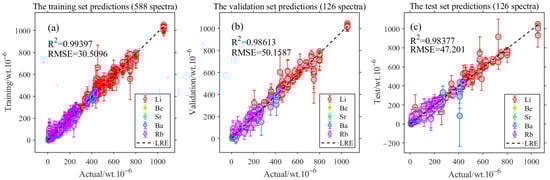
Figure 9.
Quantitative prediction of minor and trace elements based on MDS-BPNN model: (a) quantification effect of minor and trace elements in the training set; (b) quantification effect of minor and trace elements in the validation set; (c) quantification effect of minor and trace elements in the test set.
To further compare the predictive effects of BPNN quantitative analysis on five minor and trace elements, the predicted results of the test set were statistically analyzed separately by element category, as shown in Figure 10. The results showed that except for Be and Sr, the R2 of the quantitative analysis results for the other three elements were all better than 0.8, and the RMSE was better than 50. The R2 of the quantitative analysis results for Be and Sr were 0.425 and 0.514, respectively, and the RMSE were 3.936 and 9.88, respectively. The content of Be and Sr in 28 types of CRMs is relatively low, resulting in insignificant characteristics in LIBS spectra. In high-dimensional data (spliced curves), the extracted features of these two elements are not apparent, so the predictive effect of BPNN quantitative analysis on these two elements is average. Figure 10f–j were comparison diagrams of residual error and reference value uncertainty predicted by quantitative analysis of BPNN of minor and trace elements.
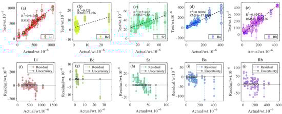
Figure 10.
Quantitative prediction of five minor and trace elements in the test set based on MDS-BPNN model: (a) quantification effect of Li; (b) quantification effect of Be; (c) quantification effect of Sr; (d) quantification effect of Ba; (e) quantification effect of Rb; (f) residual and uncertainty of Li; (g) residual and uncertainty of Be; (h) residual and uncertainty of Sr; (i) residual and uncertainty of Ba; (j) residual and uncertainty of Rb.
3.4. Identification and Quantitative Analysis of Fluoroapatite in SS
Each type of MMP randomly detected five points, and each point obtained 30 spectra, meaning that each type of MMP collected 150 spectra. Figure 11a shows the average spectrum of 150 spectra for each of the 24 MMPs, Figure 11b shows the intensity of atomic peaks of phosphorus with concentration, and Figure 11c shows the intensity of CaF molecular emission spectrum with F concentration. The key to finding fluorapatite (Ca5F(PO4)3) in SSs is the quantification of calcium, phosphorus and fluorine. The abundance of Ca can be predicted by the quantitative model of major element oxides of MDS-BPNN, and the results are shown in Figure 12a. The quantification of phosphorus and fluorine elements can refer to the process of establishing trace element quantification, which involves constructing a quantitative prediction model for phosphorus and fluorine element abundance through splicing characteristic spectral peaks. The results are shown in Figure 12b–f.
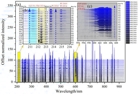
Figure 11.
LIBS-MLIF spectra of 21 MMPs: (a) LIBS-MLIF spectra of 21 MMPs; (b) LIBS-MLIF in the 210–216 nm range; (c) LIBS-MLIF in the 594–608 nm range.
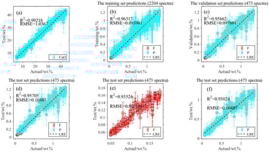
Figure 12.
Quantitative prediction of CaO, F and P elements based on MDS-BPNN model: (a) Quantitative prediction of CaO in MMPs based on MDS-BPNN model; (b) quantification effect of F and P elements in the training set; (c) quantification effect of F and P elements in the validation set; (d) quantification effect of F and P elements in the test set; (e) quantification effect of F in the test set based on MDS-BPNN model; (f) quantification effect of P in the test set based on MDS-BPNN model.
The average spectrum of MMPs in Figure 11 shows a positive correlation between element abundance and peak intensity. As element abundance increases, the intensity of the atomic or molecular emission spectra they produce also increases. However, this weak signal is highly susceptible to uneven sample mixing. Therefore, the residual of the predicted values for the abundance of F and P elements in the model is relatively large.
4. Discussion
4.1. Discussion on Quantitative Analysis Results and Geological Background of CRMs
Among the eight major element oxides of 28 CRMs, the content of TiO2 is relatively low, and the LIBS characteristic peak intensity of Ti element is weaker than that of active metals. Therefore, the characteristic spectrum of Ti is not apparent in LIBS, indicating a lack of obvious characteristic information. As a result, the MDS-BPNN model has the worst predictive effect on TiO2. Although the content of CaO, MgO, K2O, and Na2O is also low, as these major elements (Ca, Mg, K, and Na) will generate strong LIBS characteristic spectra, the MDS-BPNN model has a good prediction effect on these four oxides. Figure 13a shows the boxplot of eight major element oxides abundances for 28 types of CRMs, and Figure 13b shows the boxplot of five minor and trace element abundances for 28 types of CRMs. Among these elements, the content of Be and Sr is generally low, and their characteristic spectral peaks are weak. Therefore, the quantitative analysis effect of the model on these two elements is poor.
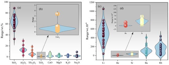
Figure 13.
Boxplots of major, minor, and trace elements content for 28 CRMs: (a) boxplot of major element oxides content for 28 CRMs; (b) boxplot of TiO2 content for 28 CRMs; (c) boxplot of minor and trace elements content for 28 CRMs; (d) boxplot of Be and Sr content for 28 CRMs.
China has a vast territory and diverse geography and climate. Therefore, this study selected 28 typical sampling areas in China. The temperature zones of the sampling areas cover the middle temperate zone, warm temperate zone, subtropical zone, tropical zone, and Qinghai Tibet Plateau. The climate characteristics of the sampling areas include temperate monsoon climate, temperate continental climate, subtropical monsoon climate, tropical monsoon climate, and plateau mountain climate. The sampling areas’ dry and wet characteristics include humid areas, arid, and semi-arid regions. Therefore, conducting laboratory research on detecting major, minor, and trace elements in CCSSs, CCFSs, and CCSs based on remote-LIBS has essential reference value for analyzing measured Martian soil data.
For the quantitative analysis results of the abundance of F and P elements, it is likely that the main factor affecting the predictive performance of the model is the uneven mixing of the two substances during the sample preparation process, which results in a certain spectral jitter in the 150 spectral data obtained for each concentration. This jitter is caused by the uneven composition of the ablated substance, as shown in Figure 14, with 3150 spliced spectra corresponding to the 21 MMPs.
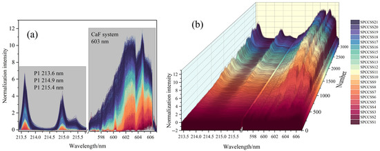
Figure 14.
Splicing of 3150 LIBS-MLIF spectral peaks from 21 MMPs; (a) splicing of LIBS-MLIF spectral peaks of F and P elements (2D); (b) splicing of LIBS-MLIF spectral peaks of F and P elements (3D).
4.2. The Significance of Searching for Biominerals in SS
Mars is the most similar planet to Earth in the solar system. Due to its rich ancient water activity and warm and humid ancient climate, Mars has always been a popular planet for human deep space exploration [33]. The ancient rivers, lakes, and deltas on Mars, rich in sediment, have become the preferred candidate areas for human probes to land on Mars and conduct patrols [34]. The Perseverance Mars rover is conducting detailed exploration in the delta intending to search for extraterrestrial life “relics” [35,36]. LIBS is a significant payload for remote analysis of mineral categories and qualitative and quantitative elements analysis. It can achieve rapid, in situ, and multi-functional detection and research and is a “sharp tool” for quickly screening potential life indicator minerals in large areas.
The complex physical and chemical matrix effects are the main factors affecting the accuracy of LIBS quantitative analysis [37]. Therefore, conducting quantitative research on major and trace elements in the geological background of CCSSs, CCFSs, and CCSs in sediments and soils has essential reference value for interpreting measured data in similar geological environments on Mars. This study focuses on 28 CRMs with Earth representative sediments and soils, demonstrating the performance and potential applications of LIBS in the rapid quantification of major, minor, and trace elements.
Life-indicating minerals are a type of biominerals that have the potential to preserve traces of life. During their formation, organisms directly or indirectly participate in the “growth” of minerals. Weathering is an essential factor affecting the preservation of Martian biominerals [38]. Assuming that this type of mineral exists on Mars and is preserved in river sediments after weathering, conducting analogical studies of the geological environment in which this type of life indicator mineral may be located in the laboratory is of great significance for discovering and identifying life indicator minerals on Mars. The results of this study prove that MLIF generated based on LIBS is an effective potential technology to identify biominerals. MLIF can carry out remote in situ rapid screening of biominerals such as fluorapatite or fluorocarbon apatite and quantitatively analyze the dusting substances formed by weathering.
4.3. The Scientific Research Value of Conducting Analogical Research on the Ground
The Martian atmosphere and water escape caused it to stop most of the chemical weathering, thus preserving the evolution process of early Mars, which has significant reference value for humans to study Mars and to help understand the early geological evolution history and origin of life on Earth [39]. Although most of the chemical weathering has stopped, the wind erosion (Martian physical weathering) caused by the collision of wind-moving particles continues to ravage the whole planet of Mars, and the physical weathering results in the exposure of fresh materials to a high radiation environment, causing a certain degree of chemical weathering [40]. Assuming that Mars experienced an evolutionary process similar to early life on Earth during warm and humid periods and produced many stromatolites, incredibly unique biological sedimentary structures such as SPs. However, under the long Martian weathering, such biological sedimentary structures exposed on the surface of Mars may gradually become dusty, thus losing the macro and micro characteristics. How to discover this type of material in SS is an important research topic for future human remote sensing in situ detection of the composition of Martian surface materials. It is expected to solve the major scientific problem of whether there has been earthlike life on Mars. It is also essential for selecting potentially significant scientific targets in sampling missions for Mars.
4.4. Limitations of Ground Simulation Experiments
For a specific geological background, ground simulation experiments can verify the application potential of LIBS-MLIF technology in the search for SPs, which can help scientists to further analyze the measured data on Mars to the maximum extent and can also provide technical reserves and references for future exploration of Mars exploration and sample-return mission to the Earth. However, ground simulation experiments inevitably have problems, such as the inherent heterogeneity of these samples. Although the samples used in the simulation experiment have undergone a series of pre-treatment, the actual Martian environment is not only cold and dry (with almost no liquid water) but also has intense radiation. The minerals on Mars have undergone a long process of chemical and physical weathering. Therefore, subsequent ground simulation experiments need to consider more factors, such as changes in chemical composition or physical properties caused by radiation.
5. Conclusions
This article applies laser-induced breakdown spectroscopy to remote detection of major, minor, and trace elements in SS. This experiment aims to evaluate the efficient remote in situ detection of SS in a large-scale area. Real-time detection of the chemical composition of SS is an important research content in fields such as geological exploration and deep space extraterrestrial life detection. Therefore, ground experiments on SS and its mixed substances containing life-indicating minerals have essential reference values for real-time detection of material composition and evaluation of potential life-indicating minerals. This article proposes a method based on MDS-BPNN combined with LIBS-MLIF to detect the composition and content of elements in SS. Taking SP as a potential indicator mineral of extraterrestrial life, it is assumed that under weathering, the macro and micromorphology of the stromatolite biological sedimentary structures disappear and become dust. The identification and quantification of SP mixed with SS are discussed for the first time, and the reference value of SP in extraterrestrial life detection is comprehensively considered.
We have demonstrated that combining MDS-BPNN with LIBS-MLIF can become a feasible method for efficiently quantifying major, minor, and trace elements in SS over a wide range of regions. In addition, we have specifically studied its potential application in deep-space extraterrestrial life detection.
We realize that in extreme extraterrestrial environments, chemical weathering can alter the specific composition of SP powder, which may lead to false negatives or false positives in identifying life-indicating minerals. This is a problem that must be considered in detecting extraterrestrial life and an essential direction for the future development of this research. We plan to conduct ground laboratory simulations of the combined effects of physical and chemical weathering in different extreme environments. In summary, the failure to consider chemical weathering may affect the determination of life-indicating minerals. But this does not negate the practicality of LIBS-MLIF technology in quantifying the abundance of F and P elements and the potential application of extraterrestrial life detection.
6. Patents
No patent.
Author Contributions
Conceptualization, H.W., X.Y., Y.X., P.F. and Y.W.; methodology, H.W., X.W., X.Y., Y.X., P.F. and Y.W.; software, H.W., X.Y., Y.X., P.F. and Y.W.; validation, H.W., X.Y., Y.X., P.F., Y.W. and S.L.; formal analysis, H.W., X.Y., Y.X., P.F., Y.W. and L.Z.; investigation, H.W. and S.L.; resources, J.J.; data curation, H.W. and J.J.; writing—original draft preparation, H.W. and X.W.; writing—review and editing, H.W. and S.L.; visualization, H.W. and J.J.; supervision, X.W., J.J. and L.Z; project administration, L.Z.; funding acquisition, X.W., J.J. and L.Z. All authors have read and agreed to the published version of the manuscript.
Funding
This research was funded by the National Natural Science Foundation of China (Grant No. U1931211, 42074210 and 42241130) and the National Key R&D Program of China (Grant No. 2021YFA0716100, 2021YFF0601201 and 2021YFF0601202) and the sponsored by Natural Science Foundation of Shanghai (Grant No. 21ZR1473700), the Shanghai Municipal Science and Technology Major Project (Grant No. 2019SHZDZX01), and the Shanghai Pilot Program for Basic Research—Chinese Academy of Science, Shanghai Branch (Grant No. JCYJ-SHFY-2021-04), the Shanghai Rising-Star Program (Grant No.21QA1409100). This work was also supported by the Pre-Research Project on Civil Aerospace Technologies (Grant No. D020102). We are grateful to Yang Ruidong and Wu Wenming from Guizhou University for their assistance and guidance in field geological sampling.
Institutional Review Board Statement
Not applicable.
Informed Consent Statement
Not applicable.
Data Availability Statement
Data underlying the results presented in this paper are not publicly available at this time but may be obtained from the authors upon reasonable request.
Conflicts of Interest
The authors declare no conflict of interest.
References
- Zou, C.H.; Mao, L.J.; Tan, Z.H.; Zhou, L.; Liu, L. Geochemistry of major and trace elements in sediments from the Lubei Plain, China: Constraints for paleoclimate, paleosalinity, and paleoredox environment. J. Asian Earth Sci. X 2021, 6, 100071. [Google Scholar] [CrossRef]
- Vital, H.; Stattegger, K. Major and trace elements of stream sediments from the lowermost Amazon River. Chem. Geol. 2000, 168, 151–168. [Google Scholar] [CrossRef]
- Carvalho, L.; Reis, A.T.; Soares, E.; Tavares, C.; Monteiro, R.J.R.; Figueira, P.; Henriques, B.; Vale, C.; Pereira, E. A Single Digestion Procedure for Determination of Major, Trace, and Rare Earth Elements in Sediments. Water Air Soil Pollut. 2020, 231, 1–14. [Google Scholar] [CrossRef]
- Chen, J.J.; Chakravarty, P.; Davidson, R.G.; Wren, D.G.; Locke, M.A.; Zhou, Y.; Brown, G.; Cizdziel, J.V. Simultaneous determination of mercury and organic carbon in sediment and soils using a direct mercury analyzer based on thermal decomposition–atomic absorption spectrophotometry. Anal. Chim. Acta 2015, 871, 9–17. [Google Scholar] [CrossRef]
- Cecile, G.; Alexandra, C.N. Microscale distribution of trace elements: A methodology for accessing major bearing phases in stream sediments as applied to the Loire basin (France). J. Soils Sediments 2020, 20, 498–512. [Google Scholar]
- Kearton, B.; Mattley, Y. Laser-induced breakdown spectroscopy: Sparking new applications. Nat. Photonics 2008, 2, 537–540. [Google Scholar] [CrossRef]
- Cremers, D.A.; Radziemski, L.J.; Wiley, J. Handbook of Laser-Induced Breakdown Spectroscopy; John Wiley & Sons: Hoboken, NJ, USA, 2006. [Google Scholar]
- Syed, K.H.S.; Javed, I.; Pervaiz, A.; Mayeen, U.K.; Sirajul, H.; Muhammad, N. Laser induced breakdown spectroscopy methods and applications: A comprehensive review. Radiat. Phys. Chem. 2020, 170, 108666. [Google Scholar]
- Zhao, S.Y.; Zhao, Y.C.; Hou, Z.Y.; Wang, Z. Rapid and high-resolution visualization elements analysis of material surface based on laser-induced breakdown spectroscopy and hyperspectral imaging. Appl. Surf. Sci. 2023, 629, 157415. [Google Scholar] [CrossRef]
- Wang, H.; Xin, Y.; Fang, P.; Jia, J.; Zhang, L.; Liu, S.; Wan, X. LIBS-MLIF Method: Stromatolite Phosphorite Determination. Chemosensors 2023, 11, 301. [Google Scholar] [CrossRef]
- Harmon, R.S.; Wise, M.A.; Curry, A.C.; Mistele, J.S.; Mason, M.S.; Grimac, Z. Rapid Analysis of Muscovites on a Lithium Pegmatite Prospect by Handheld LIBS. Minerals 2023, 13, 697. [Google Scholar] [CrossRef]
- Liu, C.; Wu, Z.; Fu, X.; Liu, P.; Xin, Y.; Xiao, A.; Bai, H.; Tian, S.; Wan, S.; Liu, Y.; et al. A Martian Analogues Library (MAL) Applicable for Tianwen-1 MarSCoDe-LIBS Data Interpretation. Remote Sens. 2022, 14, 2937. [Google Scholar] [CrossRef]
- Ribes-Pleguezuelo, P.; Guilhot, D.; Gilaberte, B.M.; Beckert, E.; Eberhardt, R.; Tünnermann, A. Insights of the Qualified ExoMars Laser and Mechanical Considerations of Its Assembly Process. Instruments 2019, 3, 25. [Google Scholar] [CrossRef]
- David, G.; Meslin, P.-Y.; Dehouck, E.; Gasnault, O.; Cousin, A.; Forni, O.; Berger, G.; Lasue, J.; Pinet, P.; Wiens, R.C.; et al. Laser-Induced Breakdown Spectroscopy (LIBS) characterization of granular soils: Implications for ChemCam analyses at Gale crater, Mars. Icarus 2021, 365, 114481. [Google Scholar] [CrossRef]
- Anderson, R.B.; Forni, O.; Cousin, A.; Wiens, R.C.; Clegg, S.M.; Frydenvang, J.; Gabriel, T.S.J.; Ollila, A.; Schröder, S.; Beyssac, O.; et al. Post-landing major element quantification using SuperCam laser induced breakdown spectroscopy. Spectrochim. Acta Part B At. Spectrosc. 2021, prepublish. [Google Scholar] [CrossRef]
- Harmon, R.S.; Senesi, G.S. Laser-Induced Breakdown Spectroscopy—A geochemical tool for the 21st century. Appl. Geochem. 2021, 128, 104929. [Google Scholar] [CrossRef]
- Chen, T.T.; Zhang, T.L.; Li, H. Applications of laser-induced breakdown spectroscopy (LIBS) combined with machine learning in geochemical and environmental resources exploration. TrAC Trends Anal. Chem. 2020, 133, 116113. [Google Scholar] [CrossRef]
- Harmon, R.S.; De, L.F.; Miziolek, A.; McNesby, K.; Walters, R.; French, P. Laser-Induced Breakdown Spectroscopy (LIBS)—An Emerging Field-Portable Sensor Technology for Real-Time, In-Situ Geochemical and Environmental Analysis. Geochem. Explor. Environ. Anal. 2005, 5, 21–28. [Google Scholar] [CrossRef]
- Senesi, G.S.; Harmon, R.S.; Hark, R.R. Field-portable and handheld laser-induced breakdown spectroscopy: Historical review, current status and future prospects. Spectrochim. Acta Part B At. Spectrosc. 2021, 175, 106013. [Google Scholar] [CrossRef]
- Delgado, T.; Fortes, F.J.; Cabalín, L.M.; Laserna, J.J. The crucial role of molecular emissions on LIBS differentiation of organic compounds of interest in astrobiology under a Mars simulated atmosphere. Spectrochim. Acta Part B At. Spectrosc. 2022, 192, 106413. [Google Scholar] [CrossRef]
- Schwieterman, E.W.; Kiang, N.Y.; Parenteau, M.N.; Harman, C.E.; DasSarma, S.; Fisher, T.M.; Arney, G.N.; Hartnett, H.E.; Reinhard, C.T.; Olson, S.L.; et al. Exoplanet Biosignatures: A Review of Remotely Detectable Signs of Life. Astrobiology 2018, 18, 663–708. [Google Scholar] [CrossRef]
- Osterhout, J.T.; Schopf, J.W.; Kudryavtsev, A.B.; Czaja, A.D.; Williford, K.H. Deep-UV Raman Spectroscopy of Carbonaceous Precambrian Microfossils: Insights into the Search for Past Life on Mars. Astrobiology 2022, 22, 1239–1254. [Google Scholar] [CrossRef] [PubMed]
- John, A.G.; Matthew, P.G.; Sharon, A.W.; Kenneth, A.F.; Ken, H.W.; Al, C. The science process for selecting the landing site for the 2020 Mars rover. Planet. Space Sci. 2018, 164, 106–126. [Google Scholar]
- Antony, J. Chapter 4–Biosignatures—The prime targets in the search for life beyond Earth. In Water World in the Solar System; Elsevier: Amsterdam, The Netherlands, 2023; pp. 167–200. [Google Scholar]
- Jonathan, D.A.C.; Carol, R.S. Searching for stromatolites: The 3.4 Ga Strelley Pool Formation (Pilbara region, Western Australia) as a Mars analogue. Icarus 2013, 224, 413–423. [Google Scholar]
- Ning, X.R.; Selesnick, I.W.; Duval, L. Chromatogram baseline estimation and denoising using sparsity (BEADS). Chemom. Intell. Lab. Syst. 2014, 139, 156–167. [Google Scholar] [CrossRef]
- Wang, H.P.; Fang, P.P.; Yan, X.R.; Zhou, Y.; Cheng, Y.; Yao, L.; Jia, J.; He, J.; Wan, X. Study on the Raman spectral characteristics of dynamic and static blood and its application in species identification. J. Photochem. Photobiol. B Biol. 2022, 232, 112478. [Google Scholar] [CrossRef]
- Fang, C.; Luo, Y.L.; Zhang, X.; Zhang, H.P.; Nolan, A.; Naidu, R. Identification and visualisation of microplastics via PCA to decode Raman spectrum matrix towards imaging. Chemosphere 2022, 286, 131736. [Google Scholar] [CrossRef]
- Dzemyda, G.; Sabaliauskas, M. Geometric multidimensional scaling: A new approach for data dimensionality reduction. Appl. Math. Comput. 2021, 409, 125561. [Google Scholar] [CrossRef]
- Wei, X.; Li, S.; Zhu, S.P.; Zheng, W.Q.; Xie, Y.; Zhou, S.L.; Hu, M.D.; Miao, Y.J.; Ma, L.K.; Wu, W.J.; et al. Terahertz spectroscopy combined with data dimensionality reduction algorithms for quantitative analysis of protein content in soybeans. Spectrochim. Acta Part A Mol. Biomol. Spectrosc. 2021, 253, 119571. [Google Scholar] [CrossRef]
- Zhang, H.; Lu, H.; Xie, F.; Ma, T.; Qian, X. Combustion Regime Identification in Turbulent Non-Premixed Flames with Principal Component Analysis, Clustering and Back-Propagation Neural Network. Processes 2022, 10, 1653. [Google Scholar] [CrossRef]
- Chen, H.; Sun, Z.; Zhong, Z.; Huang, Y. Fatigue Factor Assessment and Life Prediction of Concrete Based on Bayesian Regularized BP Neural Network. Materials 2022, 15, 4491. [Google Scholar] [CrossRef]
- Di, A.G.; Hynek, B.M. Ancient ocean on Mars supported by global distribution of deltas and valleys. Nat. Geosci. 2010, 3, 459–463. [Google Scholar]
- Stack, K.M.; Grotzinger, J.P.; Lamb, M.P.; Gupta, S.; Rubin, D.M.; Kah, L.C.; Edgar, L.A.; Fey, D.M.; Hurowitz, J.A.; McBride, M.; et al. Evidence for plunging river plume deposits in the Pahrump Hills member of the Murray formation, Gale crater, Mars. Sedimentology 2018, 66, 1768–1802. [Google Scholar] [CrossRef]
- Tarnas, J.D.; Stack, K.M.; Parente, M.; Koeppel, A.H.D.; Mustard, J.F.; Moore, K.R.; Horgan, B.H.N.; Seelos, F.P.; Cloutis, E.A.; Kelemen, P.B.; et al. Characteristics, Origins, and Biosignature Preservation Potential of Carbonate-Bearing Rocks Within and Outside of Jezero Crater. J. Geophys. Res. Planets 2021, 126, e2021JE006898. [Google Scholar] [CrossRef] [PubMed]
- Hickman-Lewis, K.; Moore, K.R.; Hollis, J.J.R.; Tuite, M.L.; Beegle, L.W.; Bhartia, R.; Grotzinger, J.P.; Brown, A.J.; Shkolyar, S.; Cavalazzi, B.; et al. In Situ Identification of Paleoarchean Biosignatures Using Colocated Perseverance Rover Analyses: Perspectives for In Situ Mars Science and Sample Return. Astrobiology 2022, 22, 1143–1163. [Google Scholar] [CrossRef] [PubMed]
- Borduchi, L.C.L.; Milori, D.M.B.P.; Meyer, M.C.; Villas-Boas, P.R. Reducing matrix effects on the quantification of Ca, Mg, and Fe in soybean leaf samples using calibration-free LIBS and one-point calibration. Spectrochim. Acta Part B At. Spectrosc. 2022, 198, 106561. [Google Scholar] [CrossRef]
- Bak, E.N.; Larsen, M.G.; Jensen, S.K.; Nørnberg, P.; Moeller, R.; Finster, K. Wind-Driven Saltation: An Overlooked Challenge for Life on Mars. Astrobiology 2019, 19, 497–505. [Google Scholar] [CrossRef]
- Jakosky, B.M. Atmospheric Loss to Space and the History of Water on Mars. Annu. Rev. Earth Planet. Sci. 2021, 49, 71–93. [Google Scholar] [CrossRef]
- Fornaro, T.; Steele, A.; Brucato, J.R. Catalytic/Protective Properties of Martian Minerals and Implications for Possible Origin of Life on Mars. Life 2018, 8, 56. [Google Scholar] [CrossRef]


Disclaimer/Publisher’s Note: The statements, opinions and data contained in all publications are solely those of the individual author(s) and contributor(s) and not of MDPI and/or the editor(s). MDPI and/or the editor(s) disclaim responsibility for any injury to people or property resulting from any ideas, methods, instructions or products referred to in the content. |
© 2023 by the authors. Licensee MDPI, Basel, Switzerland. This article is an open access article distributed under the terms and conditions of the Creative Commons Attribution (CC BY) license (https://creativecommons.org/licenses/by/4.0/).