Abstract
The Raman spectroscopy analysis technique has found extensive applications across various disciplines due to its exceptional convenience and efficiency, facilitating the analysis and identification of diverse substances. In recent years, owing to the escalating demand for high-efficiency analytical methods, deep learning models have progressively been introduced into the realm of Raman spectroscopy. However, the application of these models to portable Raman spectrometers has posed a series of challenges due to the computational intensity inherent to deep learning approaches. This paper proposes a lightweight classification model, named RepDwNet, for identifying 28 different types of biological blood. The model integrates advanced techniques such as multi-scale convolutional kernels, depth-wise separable convolutions, and residual connections. These innovations enable the model to capture features at different scales while preserving the coherence of feature data to the maximum extent. The experimental results demonstrate that the average recognition accuracy of the model on the reflective Raman blood dataset and the transmissive Raman blood dataset are 97.31% and 97.10%, respectively. Furthermore, by applying structural reparameterization to compress the well-trained model, it maintains high classification accuracy while significantly reducing the parameter size, thereby enhancing the speed of classification inference. This makes the model more suitable for deployment in portable and mobile devices. Additionally, the proposed model can be extended to various Raman spectroscopy classification scenarios.
1. Introduction
Blood, as one of the most crucial biological fluids in organisms, possesses unique characteristics in carrying biological and genetic information that other bodily fluids lack. It has found broad applications and achieved significant research outcomes in various fields such as biopharmaceuticals, species detection, and forensic exploration. Given the distinctive nature of blood products, countries have successively established corresponding legal regulations to combat illegal activities such as the smuggling of blood products. Consequently, the rapid identification of illicit blood products during import and export has become an urgent issue requiring resolution. Researchers such as H. Inouel [1] have successfully differentiated blood samples from primates and non-primates using High-Performance Liquid Chromatography (HPLC). Although this approach has yielded remarkable results, it is essential to note that it involves complex preprocessing of blood samples and demands a high level of experimental environment control. On another front, Espinoza [2] and colleagues have achieved significant classification results in distinguishing blood samples from birds, reptiles, and mammals using Mass Spectrometry (MS). Additionally, Dalton [3] and others have employed DNA analysis technology in identifying blood samples from wild animals, particularly playing a crucial role in combating poaching activities. However, both of these approaches impose high requirements on sample quality and necessitate specialized knowledge during the detection process. Consequently, the three mentioned detection methods cannot provide a quick and non-destructive inspection of samples during import and export. Overcoming the challenges of non-destructive and rapid detection for large sample datasets has become a pressing research direction that urgently needs breakthroughs.
Raman spectroscopy is a method employed for collecting spectroscopic data, acquiring specific information by recording spectral lines induced by molecular vibrations in the sample under optical excitation. Due to the diverse molecular structures of different substances, Raman spectra exhibit unique characteristics. Its advantages, including convenience, speed, and non-destructiveness, have led to widespread applications and high acclaim in disciplines such as medicine [4,5], chemistry [6,7,8], and biology [9,10]. It is noteworthy that peak information plays a crucial role in spectral data, containing key details about the molecular structure and chemical composition of the sample. In the early 1970s, scholars such as Goheen [11] delved into the impact of artificial red blood cell membrane peripheral proteins on Raman spectroscopy, achieving significant research outcomes. However, the equipment and detection methods of that time were relatively primitive, and the detection process was cumbersome, limiting its applicability in practical work environments. Subsequently, researchers gradually deepened their exploration of Raman spectroscopy in blood. It was not until the 21st century that Raman spectroscopy found extensive application in blood data analysis. In 2008, Saade [12] and colleagues successfully employed a near-infrared Raman spectroscopy approach combining Principal Component Analysis (PCA) with Mahalanobis distance to identify Hepatitis C virus in human serum, effectively classifying 24 blood samples. This experiment validated the feasibility of machine learning in Raman spectroscopy detection of blood, although the study did not incorporate preprocessing operations such as denoising on the blood dataset, potentially rendering the experimental results susceptible to noise and other factors. Simultaneously, overreliance on feature extraction methods similar to Principal Component Analysis (PCA) entails the risk of human intervention, potentially causing the omission of critical microscopic feature information in spectral data. In 2018, Kyle C. Doty [13] and colleagues successfully utilized Partial Least Squares Discriminant Analysis (PLS-DA) to distinguish blood from 17 different organisms, including humans, providing crucial assistance for forensic investigations at crime scenes and paving the way for future research into differentiating blood data from various organisms. Subsequently, researchers such as Wang [14] applied the Support Vector Machine (SVM) method to successfully inspect the blood spectral data of four avian species, offering a novel solution for analyzing the presence of food additives in blood. However, traditional machine learning algorithms often fail to achieve the expected results when handling large sample datasets. Hence, the search for a convenient, rapid, and precise Raman spectroscopy detection method becomes imperative.
With the rapid development in the field of artificial intelligence, deep learning techniques have found extensive applications across various disciplines, including Raman spectroscopy classification. The application of deep learning in Raman spectroscopy classification has yielded significant research outcomes. Currently, mainstream spectral classification methods primarily involve the utilization of one-dimensional feedforward neural networks for Raman spectral feature extraction and classification. Building upon this foundation, Dong et al. [15] successfully devised a one-dimensional convolutional neural network for distinguishing between human and animal blood, achieving efficient classification of human, dog, and rabbit blood with an accuracy of 96.33%. In their study, the authors emphasized the importance of data denoising and baseline correction and introduced unique modules to implement these steps. In comparison to traditional machine learning methods such as Support Vector Machines (SVM) and Partial Least Squares Discriminant Analysis (PLSDA), this research indicates that convolutional neural networks exhibit superior performance. This study provides valuable insights for further exploration in related fields. Huang et al. [16] designed a hierarchical convolutional neural network, achieving an average accuracy of 97% in a blind test involving 20 different animal species. Additionally, Chen et al. [17] combined a convolutional neural network with the Stochastic Gradient Descent (SGD) optimizer, achieving significant results in differentiating 19 types of blood in experiments. The model in this study demonstrated a recognition accuracy as high as 98.79%, establishing a solid foundation for research in trace blood analysis. These research achievements offer robust support for subsequent scholars engaged in trace blood studies. It is noteworthy that, in the aforementioned three experiments, no manual extraction of feature information from the data was employed. This further underscores the superiority of combining deep learning with Raman spectroscopy. From the experimental results, this approach not only yielded significant research outcomes but also exhibited superior performance compared to traditional machine learning methods. Therefore, the integration of deep learning with Raman spectroscopy presents a viable approach to overcoming challenges in the non-destructive and rapid detection of large-sample data.
Convolutional operations play a crucial role in deep learning models. However, the significant variability in peak widths observed in different Raman spectral datasets poses a challenge for traditional single-sized convolutional kernels to adequately capture information across various peak widths. Therefore, one of the primary challenges in the current field of spectral classification is achieving compatibility of convolutional kernels with information from peaks of different widths. In this context, the adoption of a multi-scale convolutional kernel strategy becomes imperative. To address this issue, Ding [18] and colleagues successfully designed a multi-scale convolutional neural network. This model adopts a cascaded hierarchical structure, utilizing three convolutional kernels of different sizes to extract more refined feature information from input spectral data, achieving a classification accuracy of 96.77%. This effectively demonstrates compatibility with peak information of different widths. The study substantiates the rationality of employing multi-scale convolutional kernels for feature extraction in Raman spectra and provides valuable directions for future research. Similarly, Den [19] and collaborators proposed an adaptive-scale deep learning model. This model achieved accuracies of 86.7% and 98% in the classification of 30 isolates and eight empirical treatment tasks, respectively, in bacterial Raman spectral classification. The performance of this model confirms the superiority of multi-scale models over both single convolutional kernel deep learning models and traditional machine learning algorithms. These studies offer directions for overcoming the challenge of effectively capturing information from peaks of different widths. However, the introduction of multi-scale models inevitably increases the model parameters, posing challenges for deployment on certain portable devices. Additionally, Raman spectra, as a type of remote sensing data with coherent information features, may suffer from a loss of feature coherence to some extent during traditional convolutional operations. Consequently, preserving feature coherence during the process of extracting feature information becomes a crucial problem that urgently needs addressing. To tackle the aforementioned issues, we propose a model named RepDwNet. This model effectively integrates local information without increasing model parameters. Experimental results demonstrate that the RepDwNet model achieves classification-balanced accuracies of 97.17% and 97.31% on transmissive and reflective blood Raman spectral datasets, respectively, showcasing its outstanding performance in blood Raman spectral classification tasks.
2. Materials and Methods
2.1. Equipment and Data Acquisition
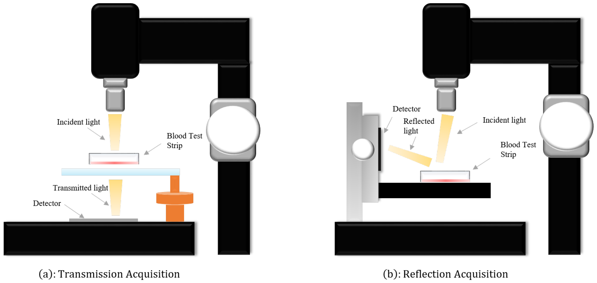
In this study, we utilized two independent Raman spectroscopy datasets, both acquired through the Surface-Enhanced Raman Scattering (SERS) strategy, with support from Beijing Huatai Nova Detection Technology Co., Ltd.,Beijing, China. To enhance the long-term sensitivity of SERS bands and facilitate the operational convenience of detection, we employed synthetically prepared silver nanoparticle (AgNP) and gold nanoparticle (AuNP) test papers for sample collection. These are surface-enhanced composite test papers that incorporate two materials, AgNPs and AuNPs. The composite surface-enhanced material paper demonstrates outstanding performance, effectively capturing information carried by materials enhanced with AgNPs or AuNPs. This significantly enhances the convenience of surface-enhanced Raman detection. It is noteworthy that, under identical testing conditions, this enhancement not only achieves or surpasses higher values compared to individual materials but also transcends a simple weighted average of AgNP and AuNP material proportions. This composite surface-enhanced material paper successfully inherits the enhancement effects of both AgNPs and AuNPs. To better address each distinct blood sample, the ratio of AgNPs to AuNPs should be adjusted within the range of 1:4 to 4:1. The detailed preparation process can be found in the relevant research literature by Wang et al. [20]. Prior to SERS testing, we rapidly heated the test papers to 65 degrees Celsius and swiftly immersed them in the sample bottle for 5 s to achieve rapid drying of the papers. It is noteworthy that we diluted the collected blood with a 0.9% NaCl solution by a factor of 10 to obtain the final sample solution. During the testing phase, the profound impact of laser-induced thermal accumulation on dark whole blood samples has been observed, leading to combustion and damage. Hence, the indispensability of employing dilution techniques to mitigate the extent of laser-induced thermal accumulation. Subsequently, we placed the moistened test papers in a microheater at 65 degrees Celsius and baked them for 1 min. Throughout the sampling process, we repeated the above steps multiple times to gradually accumulate the concentration of the target molecules in the material. For better preservation of blood specimens, we chose trisodium citrate as an anticoagulant and stored the blood at−20 degrees Celsius. During the acquisition of spectral data, we employed a portable handheld Raman spectrometer (model CR-2000, HT-NOVA Ltd., Beijing, China). To acquire high-quality blood spectral data, we employed a portable handheld Raman spectrometer (model CR-2000, HT-NOVA Limited) for the collection of spectral data. Utilizing the transmissive and reflective properties of laser light, we collected two distinct Raman spectral datasets, namely reflective and transmissive, as illustrated in Figure 1. During the data acquisition process, a laser with a power of 5 mW and a wavelength of 785 nm was utilized. Additionally, spectral data collection was complemented by scanning electron microscopy (FE-SEM, SUPRA 55, Carl Zeiss, Germany) and transmission electron microscopy (Tecnai F30, FEI company, Hillsboro, OR, USA). The signal range for reflective Raman spectra was 200–2998 cm−1, while that for transmissive Raman spectra was 166–2084 cm−1. Simultaneously, we ensured that the spectral resolution remained within the range of 4–6 cm−1. Furthermore, the pertinent parameters of the optical filter can be found in Table 1.

Figure 1.
(a) The procedures for acquiring transmissive Raman spectra by harnessing the transparency of light. (b) The steps involved in obtaining reflective Raman spectra through the utilization of the reflectivity of light.

Table 1.
The pertinent parameters of the optical filter.
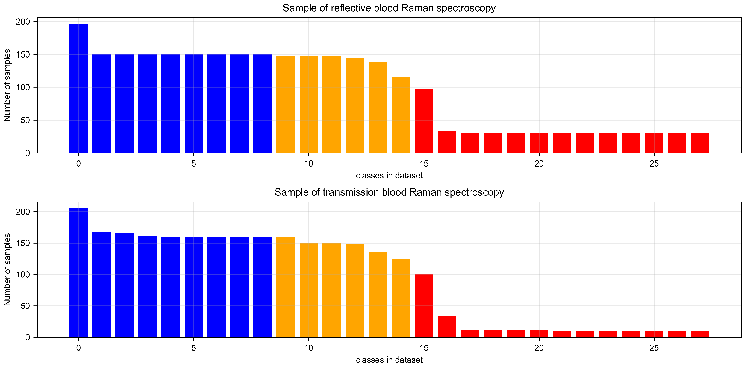
Through the aforementioned procedures, we successfully obtained two distinct sets of animal blood sample data, comprising specimens from 28 different animal species. Specifically, the reflective blood dataset comprises a total of 2696 data samples, while the transmissive blood dataset contains 2620 data samples. However, due to challenges in collecting blood samples from certain specific animals, such as pandas and golden snub-nosed monkeys, both datasets exhibit varying degrees of sample imbalance. The sample distribution of these two datasets is illustrated in Figure 2. Refer to the detailed sample categories and corresponding data in Supplementary Tables S1 and S2 for additional materials.

Figure 2.
The presented figures illustrate the statistical distribution of the reflective and transmissive animal blood datasets, respectively. In the graphs, the categories represented by the blue histograms indicate species with sample counts exceeding 150, the yellow histograms represent species with sample counts between 100 and 150, and the red histograms reflect the number of species with sample counts below 100.
2.2. Data Proccessing
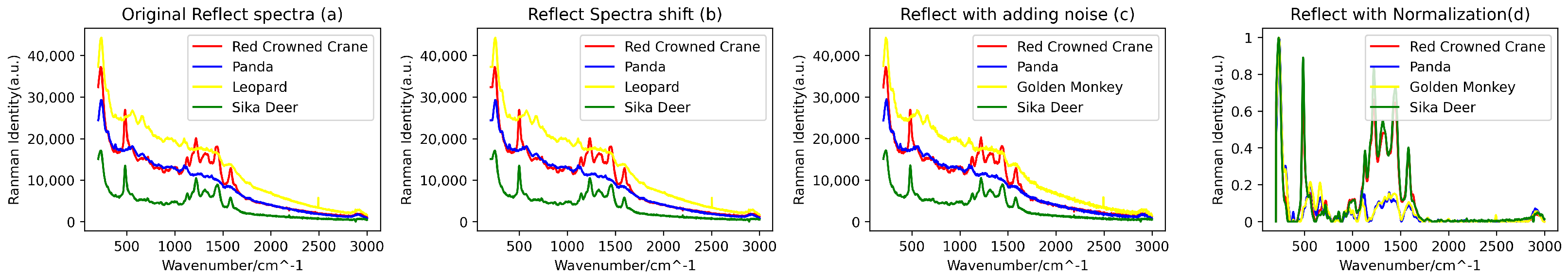
In consideration of the potential interference from external factors, such as the quality of the filter used during blood data collection, to ensure higher data quality and information accuracy, a series of data preprocessing steps were undertaken. Firstly, we employed the Savitzky–Golay filtering algorithm (with a window size of 11 and an order of 3) to perform denoising on the raw spectral data. Subsequently, a combination of the BaselineRemoval library and the Adaptive Iteratively Reweighted Penalized Least Squares (airPLS) algorithm proposed by Zhang [21] was utilized for baseline correction and fluorescence reduction in the spectral data. Additionally, due to the possibility of data point loss under varying conditions during the spectral data acquisition process, resulting in discrepancies in the lengths of spectral data for different biological species, a downsampling technique was employed. This involved uniform sampling of the spectral curves with a fixed step size (step size of 2), thus achieving uniformity in the length of the spectral data. Following the completion of downsampling, the spectral range for reflectance blood spectra covered the range of 200–2998 cm−1, while the range for transmittance blood spectra covered 166–2084 cm−1. Furthermore, to ensure the stability and reliability of the training model, the spectral data were subjected to min-max normalization. This step aimed to reduce the adverse effects of outliers on the model’s training performance, ultimately enhancing its generalization capability. Figure 3 and Figure 4 illustrate a portion of the preprocessed and augmented spectral data.
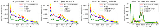
Figure 3.
(a) Original reflective blood Raman spectroscopy, (b) transformed spectra following spectral shifts, (c) introduced noise effects, and (d) reflective spectra subjected to normalization and downsampling processes.
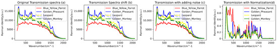
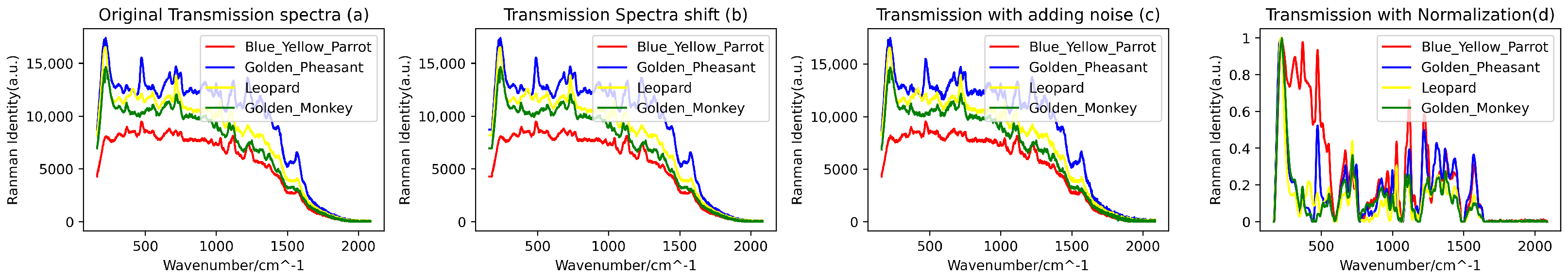
Figure 4.
(a) Original transmissive blood Raman spectroscopy, (b) transformed spectra following spectral shifts, (c) introduced noise effects, and (d) transmissive spectra subjected to normalization and downsampling processes.
2.3. Extending Dataset
The high-quality dataset plays a crucial role in facilitating the comprehensive absorption of feature information by models. It has the capability to effectively enhance the model’s generalization ability and, to a certain extent, prevent overfitting. Additionally, this training approach, built upon a high-quality dataset, aids deep learning models in acquiring a more profound understanding of complex baseline information. As illustrated in Figure 2, both datasets exhibit varying degrees of sample imbalance, which proves to be detrimental to the model’s ability to learn intrinsic feature information within Raman spectra. Therefore, to ensure the model adequately absorbs feature information, data augmentation becomes an indispensable step.
This paper’s approaches draw upon methodologies outlined in the existing literature [22,23], primarily encompassing the introduction of random Gaussian noise and the application of spectral data shifting techniques. Regarding the treatment of spectral data shifting, it is worth noting that excessive shifts can potentially result in the loss of pivotal information inherent in the original spectral data. To address this concern, a judicious choice was made to employ uniformly distributed random variables within the range of cm−1 to 16 cm−1, thereby effecting minor perturbations in the spectral data through shifts of negligible magnitude. For handling data situated at the dataset’s periphery, a decision was made to employ neighboring values for padding, thereby upholding the continuity of the dataset. Introducing Gaussian noise plays a pivotal role in the context of the signal-to-noise ratio (SNR). The signal-to-noise ratio is a crucial metric for assessing the relative strength or quality of a signal in the presence of noise. It is typically quantified as the ratio of signal power to noise power, expressed in decibels (dB). The specific mathematical expression is represented by Equation (1). It is imperative to note that the signal-to-noise ratio (SNR) values utilized in this manuscript are set at 40.
is the signal power of input data, expressed as the mean square value of the data. Expanding upon , we can obtain where N represents the total number of data points in the input spectral signal, and denotes the intensity of the data point at the corresponding index. denotes the power of noise. Equation (2) can be obtained by transforming Equation (1) through appropriate adjustments.
By squaring the , we obtain the numerical value . Ultimately, Gaussian noise with a mean of 0 and a standard deviation of is added to the original spectral data to achieve the purpose of data augmentation.
To ensure the reliability of the final experimental results, we performed sample division for two blood datasets that had not undergone data augmentation, with an approximate ratio of 8:2. Specifically, 20% of the sample data were reserved as the final test dataset, comprising 535 test samples for the reflective blood dataset and 519 test samples for the transmissive blood dataset. Subsequently, data augmentation was applied to the remaining 80% of the sample data. In practical implementation, we employed two augmentation schemes with equal probability to expand the dataset. Real data were introduced for enhancement through uniform sampling. In the augmentation of the reflective blood dataset, the sample count for each class was increased to 195. As a result, the overall sample size of the reflective blood dataset (including test data) increased from 2696 to 5995. In the case of the transmissive blood dataset, the sample count for each class was augmented to 187, leading to an increase in the overall sample size of the transmissive blood dataset (including test data) from 2620 to 5755. Table 2 summarizes the basic information of the datasets used in this study and the corresponding processing methods. It is imperative to emphasize that, owing to the distinctive characteristics inherent in the original spectra, this paper endeavors to perform expansion operations on preprocessed spectral data. The objective is to maximize the retention of the intrinsic spectral features during this process.
Table 2.
Summary of information about related datasets.
2.4. Dataset Partitioning
K-fold cross validation is widely adopted in Raman spectroscopy detection experiments [24]. This method divides the dataset into K equally sized and mutually exclusive sub-datasets to ensure consistent data sample distribution within each sub-dataset. In each validation round, K-1 sub-datasets are combined as the training set, while the 1 remaining sub-dataset serves as the test set for experimentation. This approach yields K different combinations of training and test sets, resulting in K distinct experimental outcomes. This strategy maximizes the utilization of data information while mitigating the impact of sample distribution imbalance on experimental results.
In the specific experiment, in order to make the model more reliable, we divided the augmented reflection blood dataset and transmission blood dataset in the form of 9:1. It should be noted that, as mentioned in Section 2.2, since we had divided the test set in advance, this part of the dataset for k-fold cross validation did not include the validation set. Therefore, in the overall experiment process, for the reflective blood dataset, a total of 4928 data were used for training, 532 data were used for validation, and 535 data were used for testing. For the transmission blood dataset, there are 4732 data for training, 504 data for validation, and 519 data for testing. Table 3 summarizes the fundamental aspects of dataset partitioning.
Table 3.
Summary of dataset partitioning.
2.5. Establishment of RepDwNet Model
2.5.1. Overview of RepDwNet
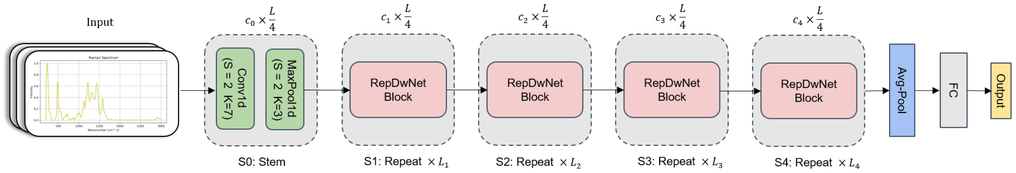
This section provides a detailed exposition of a one-dimensional convolutional neural network (CNN) model applied to Raman spectroscopy blood categorization. As shown in Figure 5, the holistic architecture of the model consists of the Stem layer, the Average Pooling layer, the Fully Connected layer, and multiple Replicated Depthwise Block (RepDwBlock) modules. In the diagram, the quantities of RepDwBlock modules are denoted as , , , and with values of 2, 2, 4, and 1, respectively. Regarding feature extraction, the spectral data are initially subjected to preliminary feature extraction via the Stem layer. The Stem layer encompasses a one-dimensional convolutional layer (Conv1D) and a maximum pooling layer (MaxPool1D), with kernel sizes of 7 and 3 and strides of 1 each. Subsequently, through the integration of four RepDwBlock modules, deep feature extraction is applied to the output of the Stem layer, incorporating residual connections to ensure coherence in feature information extraction. Ultimately, spectral data classification is accomplished by means of the Average Pooling layer and Fully Connected layer. Throughout different stages of feature extraction, the dimensional progression of the input feature sequence is (1, 16, 32, 64, 128). During the deployment phase of the model, structural reparameterization techniques were employed to amalgamate multiple branches, simplifying the model structure and rendering it more amenable for deployment on resource-constrained devices. This optimization further enhances the applicability and lucidity of the model.
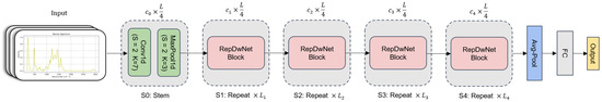
Figure 5.
The overall architecture of RepDwNet exhibits a stratified and phased design. The framework is demarcated into five successive feature extraction stages, with the latter four stages being composed of a sequence of RepDwBlock modules, while the initial stage encompasses a Stem layer. The ultimate two layers are allocated for the purpose of feature classification tasks. For the sake of brevity, the diagram omits the inclusion of normalization and activation layers.
2.5.2. RepDwNetBlock
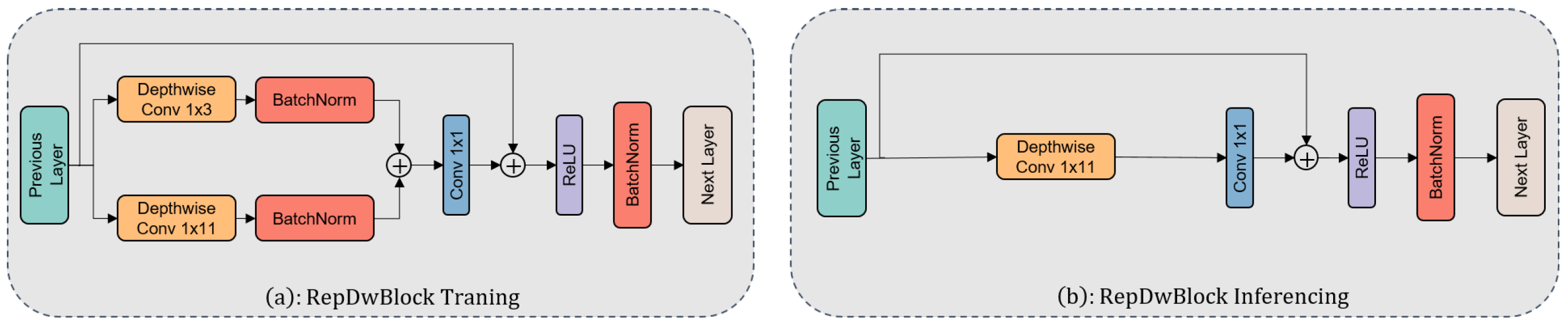
The extraction of core features in the model is undertaken by the RepDwBlock module. The design objective of this module is to integrate multi-scale convolutional kernels to endow the model with the capability to capture peaks of varying widths. To address the issue of parameter inflation caused by the multiple-branch convolutional kernels, this research introduces depthwise separable convolutions for model streamlining. Depthwise separable convolutions [25] find widespread application in visual tasks, breaking down the conventional convolution into depthwise and pointwise convolutions, thereby reducing parameter volume and computational load. In RepDwNet, several convolutional kernels (1 × 3, 1 × 11) undergo individual depthwise convolutions and their outputs are aggregated within specific branches. Ultimately, feature fusion is achieved through pointwise convolutions, enabling the model to effectively capture peak features of diverse widths. It is noteworthy that although depthwise separable convolutions have found extensive use in the field of visual classification, their application in spectral classification tasks remains somewhat limited. This primarily stems from the fact that while depthwise separable convolutions can reduce parameter count, they often come at the cost of decreased model accuracy. This trade-off appears unfavorable in the context of spectral classification tasks. However, the strategy adopted in this study precisely manages to counterbalance the contradiction between the accuracy improvement from introducing multi-scale features and the issue of parameter inflation. Figure 6 provides a detailed overview of the architecture of the RepDwBlock module.
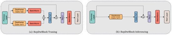
Figure 6.
(a) Module structure utilized during RepDwNet model training and (b) module structure employed during RepDwNet model testing or validation.
If confined solely to conventional convolutional operations, there is a potential loss of coherent spectral feature information to a certain extent. To effectively preserve this information to the utmost degree, respectively employs residual connection structures. The intrinsic capabilities of residual connections in addressing the issue of accuracy saturation degradation and mitigating the vanishing gradient phenomenon [23] render them extensively applicable in various deep learning models. This architectural paradigm proficiently establishes inter-layer direct connections, thereby endowing the model not only with the capacity to capture local feature information but also to retain spectral coherence. Consequently, for data possessing coherent spatial or temporal features such as Raman spectra, residual connections manifest supplementary significance.
2.5.3. Multi-Scale Reparameterization
In the context of classification tasks involving Raman spectroscopy data, models are predominantly deployed in portable devices. Inspired by models such as RepVGG [26], this study introduces structural reparameterization techniques. Through this technique, the model’s structure is simplified while maintaining its original performance, resulting in improved inference speed. This adaptation makes the model more suitable for deployment on portable devices. Structural reparameterization plays a crucial role in this paper, contributing not only to optimizing the computational efficiency of the model but also effectively maintaining predictive accuracy under the premise of achieving lightweight deployment. This section provides a detailed description of the implementation of structural reparameterization for the model.
Equations (3) and (4) represent the convolution operation and the normalization operation, respectively. In these equations, the variable X represents the input received by the operation, and b and correspond to the bias terms of the respective operations. In Equation (3), the variables , , and correspond to the mean, variance, and learnable factor of this operation, respectively. By integrating the convolution operation and batch normalization operation, they can be transformed into convolution operations with equivalent responses. Specifically, we introduce the output of the initial convolutional layer into the batch normalization layer and perform the transformation, yielding Equation (5):
It is not difficult to observe that this form can also be regarded as a convolution operation denoted as Equation (6):
In practical implementation, the fusion of convolutional kernels is achieved by laterally extending smaller convolutional kernels to match the dimensions of the largest convolutional kernel. Subsequently, the weights and biases of these kernels are aggregated, yielding a cohesive amalgamation of the convolutional kernels. In the aforementioned equation, where is defined as , can be expressed as .
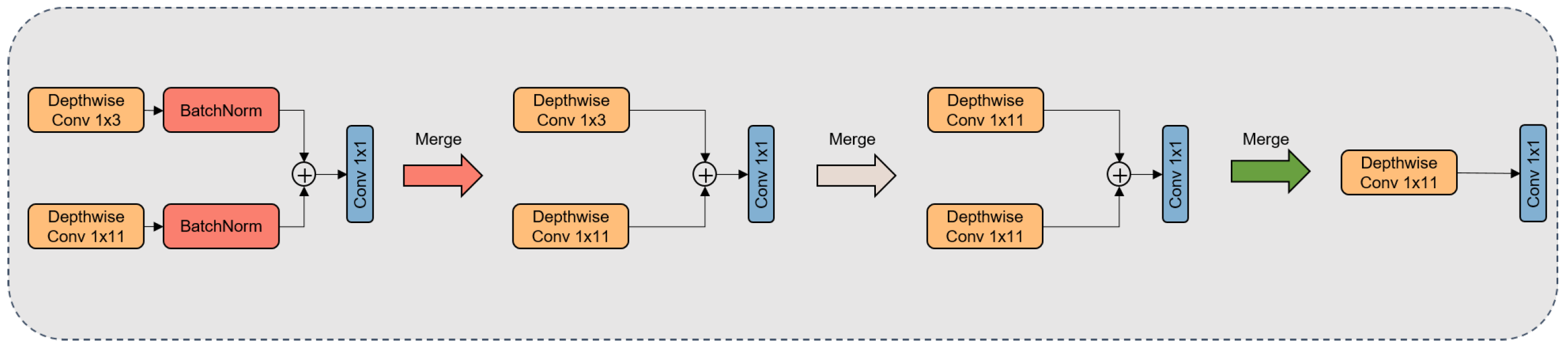
As depicted in Figure 7, we optimized the model architecture by transitioning from the original dual-branch structure to a single-branch model. Firstly, we integrated the Conv1D operation and its adjacent normalization operation (refer to Equation (5)) to form a novel convolutional operation (refer to Equation (6)). Subsequently, employing zero-padding, we expanded the 1 × 3 convolutional kernel to the left and right, extending it to a 1 × 11 configuration. Building upon this, we further amalgamated these two 1 × 11 convolutional kernels. During the merging step, a corresponding summation operation was applied to the biases and parameter matrices of the two convolutional kernels, ultimately fusing them into a completely new 1 × 11 convolutional kernel. The objective of these structural adjustments is to enhance the model’s applicability in production environments while preserving its performance.
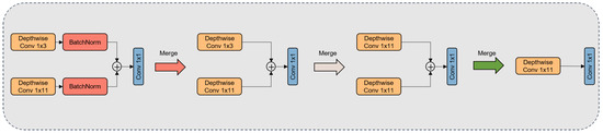
Figure 7.
The figure illustrates how dual-branch convolutional kernels undergo a fusion process to evolve into a single-branch convolutional kernel.
In practical implementation, the effective merging of convolutional kernels requires special attention to several key details. Firstly, it is essential to ensure that, prior to merging, the output dimensions of the two convolutional kernels are consistent. This is a crucial factor in ensuring the smooth progression of the model after merging. Secondly, it is necessary to maintain equal stride values for both convolutional kernels to uphold the consistency of the merging operation. This method can also be applied to convolutional kernels with sizes differing by a factor of 2. Ultimately, the model that undergoes merging enjoys a reduction in parameter requirements while preserving the same level of inference accuracy as before the merging process. This operational approach enhances model efficiency while ensuring accuracy throughout the inference process.
3. Results
3.1. Model Training
This study implemented the described model using the Python programming language and utilized core modules implemented with major frameworks such as PyTorch and scikit-learn. The model falls into the category of a classification model, and it is crucial to judiciously select a loss function and optimizer for fine-tuning its weights to achieve optimal performance. In our experiments, we employed the Adam optimizer for optimizing model parameters. Specifically, we set the learning rate of the Adam optimizer to 0.001, while configuring the exponential decay rates for the first-moment estimate () as 0.9 and the second-moment estimate () as 0.999. Furthermore, we applied an exponential decay strategy to adjust the model’s learning rate, with a decay factor of 0.95.
Taking into consideration the multi-class nature of the model, we employed the technique of one-hot encoding in conjunction with the cross-entropy loss function to quantify the disparity between the model’s predictions and the actual labels. This evaluative approach has demonstrated remarkable efficacy when addressing tasks involving multiple classification categories.
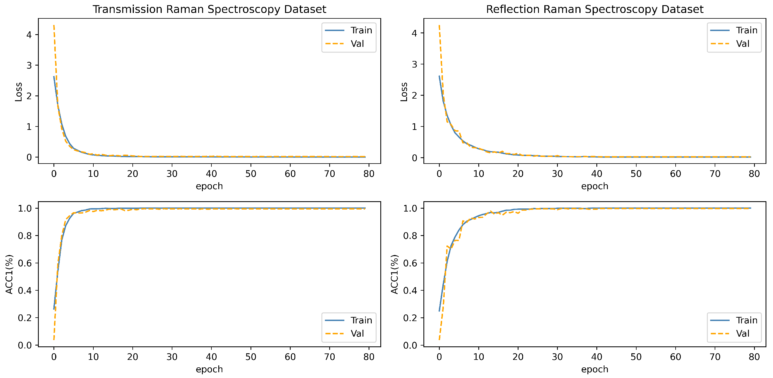
The experimentation was conducted on a server equipped with the NVIDIA GeForce RTX 4090 GPU which purchased in Shanghai, China. Throughout the experimental procedure, a batch size of 128 was employed for input data, and the model underwent 80 iterations of training. Additionally, an early stopping strategy was implemented, whereby training ceased if the model’s accuracy failed to exhibit improvement over a consecutive span of 10 epochs. Ultimately, the optimal model weight parameters, reflecting superior performance during the experimentation, were preserved for subsequent evaluative purposes. The fluctuations in metrics such as loss and accuracy during the model training process are illustrated in Figure 8.
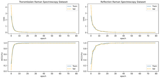
Figure 8.
The loss curve and AUC curve of the model in the training process of two blood datasets. The blue curve is the training set, and the orange curve is the validation set.
3.2. Model Evaluation
Accuracy is one of the most intuitive metrics for assessing model performance. However, when dealing with imbalanced datasets, traditional calculation methods are prone to causing the model to overly focus on the majority class, resulting in a bias in performance metrics. To provide a more objective evaluation of model performance, this study employs balanced accuracy for analysis. Balanced accuracy aims to address class imbalance issues by calculating the average sensitivity (recall) for each class and assigning equal weight to each class. It is worth noting that balanced accuracy shares conceptual similarities with macro-recall, especially in multi-class tasks, where their formulas are identical. To clearly distinguish between the two, this paper introduces the adjusted balanced accuracy, whose formula is presented in Equation (7). The adjusted balanced accuracy incorporates adjustments for randomness in the results, ensuring that a random performance scores as 0 and a perfect performance scores as 1.
Additionally, considering the presence of data imbalance in the dataset, this study employs evaluation metrics such as precision, recall, and F1-Score to comprehensively assess the model performance. Precision reflects the accuracy of positive predictions, with its value indicating the proportion of correctly predicted positive instances among all instances predicted as positive. As for recall, an increase in its numerical value signifies a stronger ability of the model to detect true positive instances. F1-Score, on the other hand, integrates both precision and recall, providing a balanced measure of the overall model performance. During the evaluation process, given the relatively limited number of true instances for certain species, the corresponding sample size in the test set is also constrained. Therefore, we adopt a macro-average approach to calculate the relevant performance metrics to maintain the comprehensiveness of the evaluation. Specifically, the formulas for computing the performance metrics are provided in Equations (8)–(10).
In the equations, , , and denote true positives, false positives, and false negatives, respectively.
During the experimental process, we employed functions provided by the sklearn library to calculate relevant performance metrics. This toolkit afforded us the necessary support, enabling the effective evaluation of experimental outcomes.
3.3. Model Performance
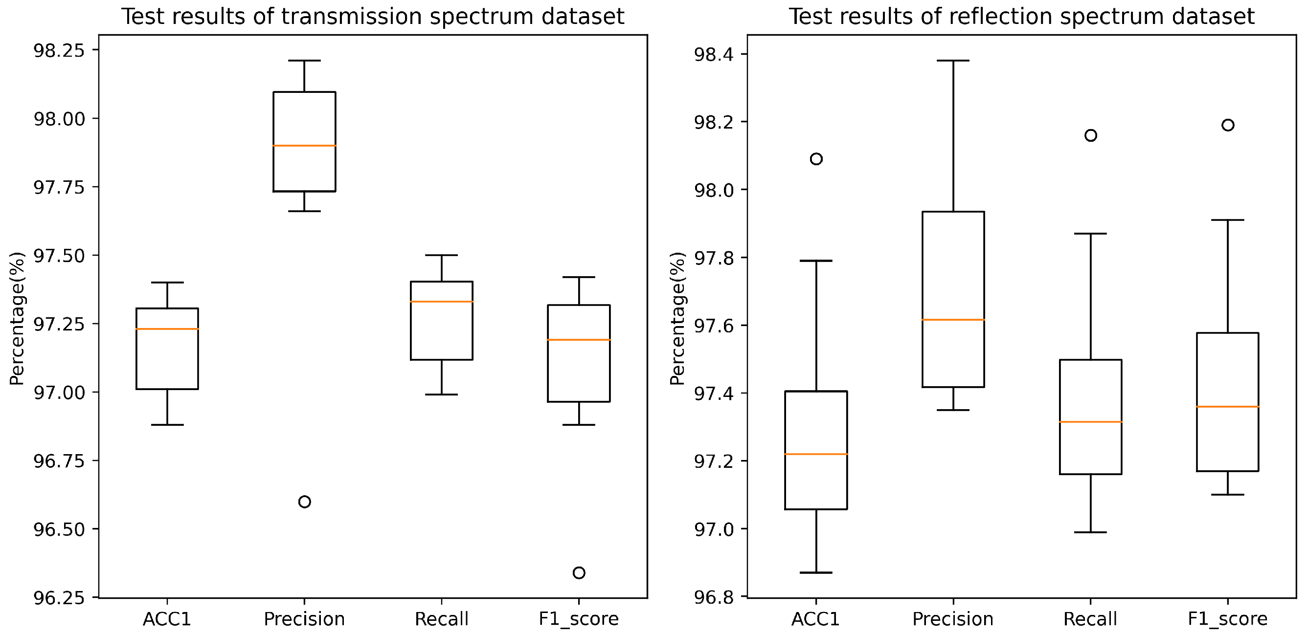
To enhance the reliability of model outcomes and mitigate the stochasticity during the model training process, this study employed a 10-fold cross-validation methodology for conducting multiple experiments while controlling the variables associated with model parameters. Throughout the experimental procedure, for each cross-validation iteration, we recorded the model’s performance metrics on the test dataset, including accuracy, precision, recall, and F1 score. A detailed depiction of the model’s performance evaluation results on two distinct datasets is presented in Figure 9. Notably, across the transmissive and reflective Raman spectroscopy datasets, the model exhibited remarkable performance, achieving balanced accuracies of 97.17% and 97.31%, respectively. It is noteworthy that, while maintaining elevated precision and recall rates, the model demonstrated significant stability. Specifically, precision values of 97.80% and 97.70%, along with recall rates of 97.27% and 97.40%, were recorded. The culmination of these high-caliber evaluation metrics signifies that the model is adept not only at accurately predicting positive samples but also at effectively identifying a substantial proportion of positive instances within the samples. Furthermore, the model achieved F1 scores of 97.09% and 97.45% on the transmissive and reflective datasets, respectively, further underscoring the well-balanced equilibrium achieved between recall and precision.
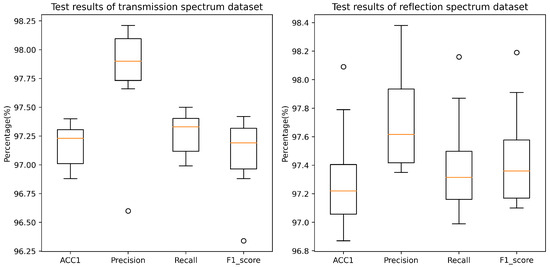
Figure 9.
Classification performance of the proposed RepDwNet model on two blood datasets. The dots in the graph represent outliers, meaning their values are significantly higher or lower compared to the other data points.
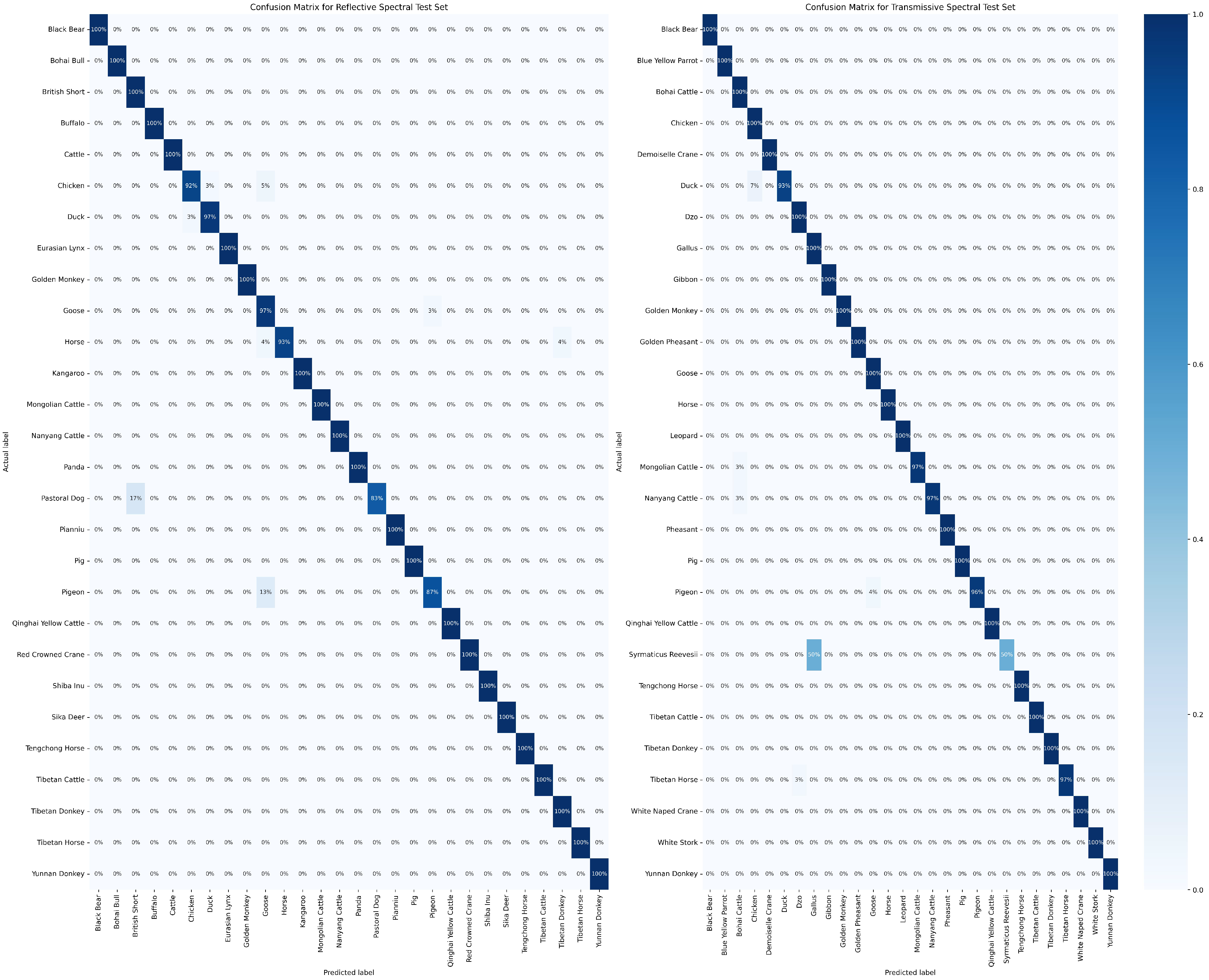
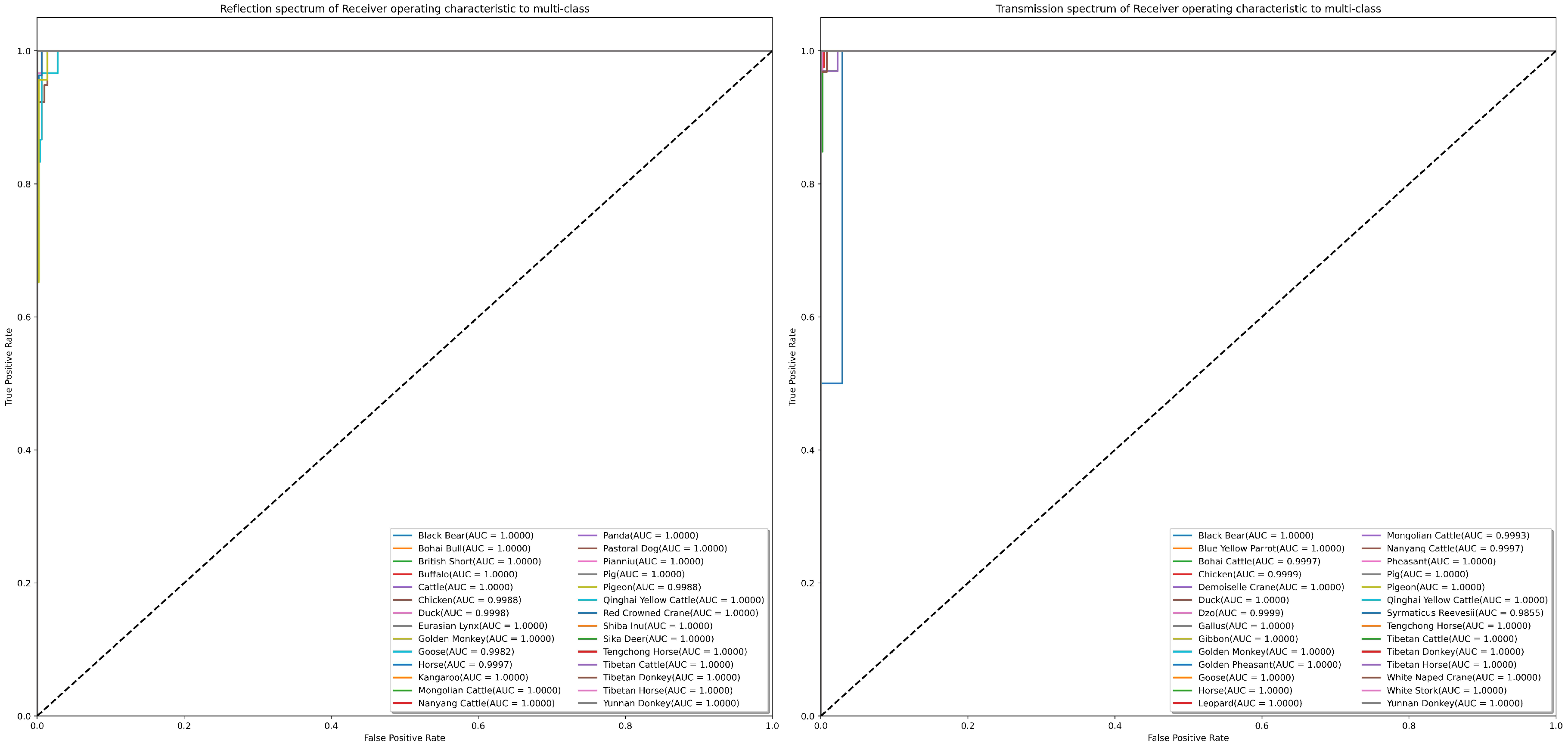
The confusion matrix is widely regarded as a valuable tool for intuitively demonstrating the classification performance of a model on different categories. In Figure 10, the results of the model’s classification predictions for two distinct test samples are presented. In this figure, the vertical axis represents the actual categories of the samples, while the horizontal axis represents the predicted sample categories. It is noteworthy that in the transmissive blood dataset, the model performs relatively poorly in classifying Syrmaticus Reevesii compared to other species. We attribute this outcome primarily to the higher requirements of this species for sample quantity and quality. Despite some degree of data augmentation, the model still struggles to fully learn more effective feature information. However, in the classification of other species, the model demonstrates excellent performance. More detailed confusion matrix data can be obtained from Tables S3 and S4 in the Supplementary Information. To further assess the sensitivity and specificity of the model’s classification results, we employ Receiver Operating Characteristic curves (ROC curves) for a more in-depth examination, as specifically presented in Figure 11. Through analysis of this figure, it becomes clear that the RepDwNet model exhibits outstanding classification efficiency in the small-sized sample dataset after data augmentation. Combining the aforementioned classification results and analysis, we have reason to believe that the classification performance of RepDWNet on the two blood datasets is reliable.

Figure 10.
The displayed figures depict the confusion matrix results of RepDwNet in two distinct blood spectral datasets. The (left) figure corresponds to the confusion matrix of transmissive blood spectral data, while the (right) figure corresponds to the confusion matrix of reflective blood spectral data.
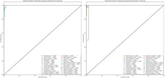
Figure 11.
The presented illustrations depict the ROC curve results of RepDwNet on two distinct blood spectroscopy datasets. The ROC curve corresponding to transmissive blood spectroscopy is shown in the (left) figure, whereas the (right) figure corresponds to the curve derived from reflective blood spectroscopy.
3.4. Comparison with Other Classification Methods
To assess the performance of Raman RepDwNet in Raman spectroscopy classification, we conducted a comparative analysis with other network classification models proposed by scholars in the last two years. These models include a one-dimensional VGG Raman spectroscopy classification network proposed by Sang [27], a model combining LSTM with convolutional neural networks proposed by Bratchenkoa [28], a one-dimensional AlexNet Raman spectroscopy classification network designed by Zhang [29], as well as a pure multi-head attention mechanism network adopted by Liu et al. [30] and an adaptive multi-scale convolutional neural network designed by Deng et al. [19]. In the process of experimental comparison, we utilized the same experimental dataset and employed a 10-fold cross-validation method. To achieve optimal classification predictive performance, we fine-tuned each model.
According to the experimental results in Table 4, RepDWNet demonstrates unique advantages in extracting blood spectral features compared to models designed by scholars such as Song, Zhang, and Liu. On both the transmissive blood dataset and reflective blood dataset, RepDWNet achieves classification-balanced accuracies of 97.17% and 97.31%, respectively. This indicates that even when facing imbalanced datasets, RepDWNet can still make accurate predictions for the majority of cases. Furthermore, the model has achieved breakthroughs in terms of parameter size and inference speed. In comparison to models designed by Bratchenko et al. [28], although RepDWNet exhibits a slightly lower inference speed, it demonstrates relatively high classification performance under a smaller memory footprint. In addition, despite not achieving a significant breakthrough in classification performance compared to the network designed by Deng et al. [19], as mentioned earlier, RepDWNet has not addressed the parameter growth issue caused by multi-scale models. While RepDWNet experiences a slight decline in classification performance, this decrease contributes to the model’s characteristics of being more lightweight and having a faster inference speed. Therefore, compared to other Raman spectroscopy classification networks on the market, RepDWNet possesses unique model performance advantages. It successfully maintains high classification performance while reducing the model’s parameter size and improving inference speed.
Table 4.
The present study presents a comparative experimental analysis of the RepDwNet model, proposed herein, with respect to Raman spectroscopy classification approaches put forth by other researchers. This comparison is conducted using transmissive and reflective blood datasets.
In addition, this study conducted a subtle evaluation of machine learning algorithms commonly used for Raman spectroscopy classification. As evidenced by the comparative results in Table 5, RepDWNet demonstrates outstanding classification performance compared to the traditional Partial Least Squares (PLS) algorithm. Furthermore, an empirical comparison was performed between RepDWNet and the combination of Principal Component Analysis (PCA) with Support Vector Machine(SVM). However, the PCA+SVM algorithm exhibited a noticeable overfitting phenomenon on the test set, despite achieving significant effectiveness on the training and validation sets. We attribute this to the possibility that PCA+SVM learned inappropriate information, during the process of acquiring blood spectral feature information. Therefore, we chose not to present the experimental results of PCA+SVM in the table. Consequently, from a comprehensive perspective, RepDWNet demonstrates unique superiority in extracting feature information from blood Raman spectra.
Table 5.
The table presented herein illustrates a comparative analysis between RepDWNet and selected mainstream machine learning algorithms.
4. Conclusions
In this study, we introduce RepDWNet, a lightweight Raman spectroscopy classification network. This model combines multiple-scale convolutional kernels while maintaining a smaller model parameter size and faster inference speed. To address the coherence of Raman spectroscopy, we incorporate residual connections to facilitate inter-layer information transfer. Simultaneously, to enhance the model’s suitability for portable devices, we employ result reparameterization techniques, rendering the model more concise and expediting the inference speed. Furthermore, to better capture the intrinsic features of Raman spectra, data augmentation techniques are applied to augment two imbalanced datasets. Comprehensive experimental results demonstrate that data augmentation operations, coupled with RepDWNet, yield significant balanced accuracy on both transmissive and reflective blood datasets, achieving 97.17% and 97.31%, respectively. Through ablation experiments, we observe that, for Raman spectroscopy classification, larger convolutional kernels may outperform smaller ones, a direction we aim to thoroughly validate in future investigations. Finally, the Raman spectroscopy augmentation techniques and RepDWNet proposed in this paper can be extended to other spectral classification domains.
Supplementary Materials
The following supporting information can be downloaded at: https://www.mdpi.com/article/10.3390/chemosensors12020029/s1, Table S1: Reflective Raman spectroscopy dataset category and sample details; Table S2: Transmission Raman spectroscopy dataset category and sample details; Table S3: Classification report of Raman RepDwNet for reflective Raman spectral of blood species identification; Table S4: Classification report of Raman RepDwNet for transmission Raman spectral of blood species identification
Author Contributions
Conceptualization, J.H.; methodology, J.H. and P.R.; software, R.Z.; validation, J.H.; formal analysis, J.H., Y.L. and P.R.; investigation, S.X.; resources, R.Z.; data curation, S.X. and Y.L.; writing—original draft preparation, J.H.; writing—review and editing, Y.L. and R.Z.; visualization, J.H.; supervision, Y.L. and J.H.; project administration, R.Z.; funding acquisition, R.Z. All authors have read and agreed to the published version of the manuscript.
Funding
This research was funded by the National Key R&D Plan under Grant No. 2021YFF0601200 and 2021YFF0601204.
Institutional Review Board Statement
Not applicable.
Informed Consent Statement
Not applicable.
Data Availability Statement
Data are contained within the article.
Acknowledgments
The authors would like to thank the anonymous reviewers for their invaluable suggestions that helped improve the manuscript. We would also like to thank Yingfeng Li for her help with data curation. The biological blood protocol used in this study has been assessed and approved by the Life Science Ethics Committee of the Shanghai Institutes for Biological Sciences, Chinese Academy of Sciences (Ethics Review Approval Number: ER-SIBS-251910).
Conflicts of Interest
Authors Shengjun Xiong employed by the company HT-NOVA Co., Ltd. The remaining authors declare that the research was conducted in the absence of any commercial or financial relationships that could be construed as a potential conflict or interest.
References
- Inouel, H.; Takabe, F.; Takenaka, O.; Iwasa, M.; Maeno, Y. Species identification of blood and bloodstains by high-performance liquid chromatography. Int. J. Leg. Med. 1990, 104, 9–12. [Google Scholar] [CrossRef] [PubMed]
- Espinoza, E.O.; Lindley, N.C.; Gordon, K.M.; Ekhoff, J.A.; Kirms, M.A. Electrospray ionization mass spectrometric analysis of blood for differentiation of species. Anal. Biochem. 1999, 268, 252–261. [Google Scholar] [CrossRef] [PubMed]
- Dalton, D.L.; Kotze, A. DNA barcoding as a tool for species identification in three forensic wildlife cases in South Africa. Forensic Sci. Int. 2011, 207, e51–e54. [Google Scholar] [CrossRef] [PubMed]
- Traynor, D.; Duraipandian, S.; Bhatia, R.; Cuschieri, K.; Tewari, P.; Kearney, P.; D’Arcy, T.; O’Leary, J.J.; Martin, C.M.; Lyng, F.M. Development and validation of a Raman spectroscopic classification model for Cervical Intraepithelial Neoplasia (CIN). Cancers 2022, 14, 1836. [Google Scholar] [CrossRef] [PubMed]
- Bratchenko, I.A.; Bratchenko, L.A. Comment on “Serum Raman spectroscopy combined with multiple classification models for rapid diagnosis of breast cancer”. Photodiagn. Photodyn. Ther. 2023, 41, 103215. [Google Scholar] [CrossRef] [PubMed]
- Wang, J.; Liu, Y.; Song, P.; Fan, X.; Ma, F. Mechanism of surface plasmon-catalyzed reaction of fluorine phenylboronic acid. J. Nanophotonics 2018, 12, 036009. [Google Scholar] [CrossRef]
- Park, S.; Lee, J.; Khan, S.; Wahab, A.; Kim, M. Machine learning-based heavy metal ion detection using surface-enhanced Raman spectroscopy. Sensors 2022, 22, 596. [Google Scholar] [CrossRef]
- Theobald, N.; Ledvina, D.; Kukula, K.; Maines, S.; Hasz, K.; Raschke, M.; Crawford, J.; Jessing, J.; Li, Y. Identification of Unknown Nanofabrication Chemicals Using Raman Spectroscopy and Deep Learning. IEEE Sens. J. 2023, 23, 7910–7916. [Google Scholar] [CrossRef]
- Mo, W.; Wen, J.; Huang, J.; Yang, Y.; Zhou, M.; Ni, S.; Le, W.; Wei, L.; Qi, D.; Wang, S.; et al. Classification of Coronavirus Spike Proteins by Deep-Learning-Based Raman Spectroscopy and its Interpretative Analysis. J. Appl. Spectrosc. 2023, 89, 1203–1211. [Google Scholar] [CrossRef]
- Ho, C.S.; Jean, N.; Hogan, C.A.; Blackmon, L.; Jeffrey, S.S.; Holodniy, M.; Banaei, N.; Saleh, A.A.; Ermon, S.; Dionne, J. Rapid identification of pathogenic bacteria using Raman spectroscopy and deep learning. Nat. Commun. 2019, 10, 4927. [Google Scholar] [CrossRef]
- Goheen, S.; Gilman, T.; Kauffman, J.; Garvin, J. The effect on Raman spectra of extraction of peripheral proteins from human erythrocyte membranes. Biochem. Biophys. Res. Commun. 1977, 79, 805–814. [Google Scholar] [CrossRef]
- Saade, J.; Pacheco, M.T.T.; Rodrigues, M.R.; Silveira, L., Jr. Identification of hepatitis C in human blood serum by near-infrared Raman spectroscopy. Spectroscopy 2008, 22, 387–395. [Google Scholar] [CrossRef]
- Doty, K.C.; Lednev, I.K. Differentiation of human blood from animal blood using Raman spectroscopy: A survey of forensically relevant species. Forensic Sci. Int. 2018, 282, 204–210. [Google Scholar] [CrossRef]
- Wang, H.; Fang, P.; Yan, X.; Zhou, Y.; Cheng, Y.; Yao, L.; Jia, J.; He, J.; Wan, X. Study on the Raman spectral characteristics of dynamic and static blood and its application in species identification. J. Photochem. Photobiol. B Biol. 2022, 232, 112478. [Google Scholar] [CrossRef]
- Dong, J.; Hong, M.; Xu, Y.; Zheng, X. A practical convolutional neural network model for discriminating Raman spectra of human and animal blood. J. Chemom. 2019, 33, e3184. [Google Scholar] [CrossRef]
- Huang, S.; Wang, P.; Tian, Y.; Bai, P.; Chen, D.; Wang, C.; Chen, J.; Liu, Z.; Zheng, J.; Yao, W.; et al. Blood species identification based on deep learning analysis of Raman spectra. Biomed. Opt. Express 2019, 10, 6129–6144. [Google Scholar] [CrossRef] [PubMed]
- Chen, J.; Wang, P.; Tian, Y.; Zhang, R.; Sun, J.; Zhang, Z.; Gao, J. Identification of blood species based on surface-enhanced Raman scattering spectroscopy and convolutional neural network. J. Biophotonics 2023, 16, e202200254. [Google Scholar] [CrossRef] [PubMed]
- Ding, J.; Lin, Q.; Zhang, J.; Young, G.M.; Jiang, C.; Zhong, Y.; Zhang, J. Rapid identification of pathogens by using surface-enhanced Raman spectroscopy and multi-scale convolutional neural network. Anal. Bioanal. Chem. 2021, 413, 3801–3811. [Google Scholar] [CrossRef]
- Deng, L.; Zhong, Y.; Wang, M.; Zheng, X.; Zhang, J. Scale-adaptive deep model for bacterial Raman spectra identification. IEEE J. Biomed. Health Inform. 2021, 26, 369–378. [Google Scholar] [CrossRef] [PubMed]
- Wang, C.; Wan, Y.; Su, Y.; Cai, Y.; Xiong, S.; Yuan, D.; Xia, Z.; Zhu, J. An Expedient SERS Strip Tactic for Rapid On-Site Detection with Long-Time Sensitivity and Repeatability. Adv. Mater. Sci. Eng. 2021, 2021, 5560513. [Google Scholar] [CrossRef]
- Zhang, Z.M.; Chen, S.; Liang, Y.Z. Baseline correction using adaptive iteratively reweighted penalized least squares. Analyst 2010, 135, 1138–1146. [Google Scholar] [CrossRef]
- Zhang, W.; Feng, W.; Cai, Z.; Wang, H.; Yan, Q.; Wang, Q. A deep one-dimensional convolutional neural network for microplastics classification using Raman spectroscopy. Vib. Spectrosc. 2023, 124, 103487. [Google Scholar] [CrossRef]
- Kazemzadeh, M.; Hisey, C.L.; Zargar-Shoshtari, K.; Xu, W.; Broderick, N.G. Deep convolutional neural networks as a unified solution for Raman spectroscopy-based classification in biomedical applications. Opt. Commun. 2022, 510, 127977. [Google Scholar] [CrossRef]
- Yu, M.; Ding, J.; Liu, W.; Tang, X.; Xia, J.; Liang, S.; Jing, R.; Zhu, L.; Zhang, T. Deep multi-feature fusion residual network for oral squamous cell carcinoma classification and its intelligent system using Raman spectroscopy. Biomed. Signal Process. Control 2023, 86, 105339. [Google Scholar] [CrossRef]
- Howard, A.G.; Zhu, M.; Chen, B.; Kalenichenko, D.; Wang, W.; Weyand, T.; Andreetto, M.; Adam, H. Mobilenets: Efficient convolutional neural networks for mobile vision applications. arXiv 2017, arXiv:1704.04861. [Google Scholar]
- Ding, X.; Zhang, X.; Ma, N.; Han, J.; Ding, G.; Sun, J. Repvgg: Making vgg-style convnets great again. In Proceedings of the IEEE/CVF Conference on Computer Vision and Pattern Recognition, Nashville, TN, USA, 19–25 June 2021; pp. 13733–13742. [Google Scholar]
- Sang, X.; Zhou, R.g.; Li, Y.; Xiong, S. One-dimensional deep convolutional neural network for mineral classification from Raman spectroscopy. Neural Process. Lett. 2021, 54, 677–690. [Google Scholar] [CrossRef]
- Bratchenko, I.A.; Bratchenko, L.A.; Khristoforova, Y.A.; Moryatov, A.A.; Kozlov, S.V.; Zakharov, V.P. Classification of skin cancer using convolutional neural networks analysis of Raman spectra. Comput. Methods Programs Biomed. 2022, 219, 106755. [Google Scholar] [CrossRef] [PubMed]
- Zhang, X.; Song, X.; Li, W.; Chen, C.; Wusiman, M.; Zhang, L.; Zhang, J.; Lu, J.; Lu, C.; Lv, X. Rapid diagnosis of membranous nephropathy based on serum and urine Raman spectroscopy combined with deep learning methods. Sci. Rep. 2023, 13, 3418. [Google Scholar] [CrossRef] [PubMed]
- Liu, B.; Liu, K.; Qi, X.; Zhang, W.; Li, B. Classification of deep-sea cold seep bacteria by transformer combined with Raman spectroscopy. Sci. Rep. 2023, 13, 3240. [Google Scholar] [CrossRef]
Disclaimer/Publisher’s Note: The statements, opinions and data contained in all publications are solely those of the individual author(s) and contributor(s) and not of MDPI and/or the editor(s). MDPI and/or the editor(s) disclaim responsibility for any injury to people or property resulting from any ideas, methods, instructions or products referred to in the content. |
© 2024 by the authors. Licensee MDPI, Basel, Switzerland. This article is an open access article distributed under the terms and conditions of the Creative Commons Attribution (CC BY) license (https://creativecommons.org/licenses/by/4.0/).