
Modelling Motor Insurance Claim Frequency and Severity Using Gradient Boosting †


Abstract
:1. Introduction
2. Gradient Boosting Machines
3. Empirical Strategy
3.1. Dataset Information and Treatment
3.2. Tuning Approach
4. Results
4.1. Model Performance
4.2. Model Interpretation
4.2.1. Variable Importance Measure
4.2.2. Partial Dependence Plots
4.2.3. GLM Model Results
4.2.4. Searching for Interactions
5. Conclusions
Author Contributions
Funding
Institutional Review Board Statement
Informed Consent Statement
Data Availability Statement
Acknowledgments
Conflicts of Interest
References
- Aguero-Valverde, Jonathan. 2013. Multivariate spatial models of excess crash frequency at area level: Case of Costa Rica. Accident Analysis & Prevention 59: 365–73. [Google Scholar]
- Ashofteh, Afshin, and Jorge M. Bravo. 2021. A Conservative Approach for Online Credit Scoring. Expert Systems With Applications 176: 114835. [Google Scholar] [CrossRef]
- Ashofteh, Afshin, Jorge M. Bravo, and Mercedes Ayuso. 2022. A New Ensemble Learning Strategy for Panel Time-Series Forecasting with Applications to Tracking Respiratory Disease Excess Mortality during the COVID-19 pandemic. Applied Soft Computing 128: 109422. [Google Scholar] [CrossRef]
- Ayuso, Mercedes, Jorge M. Bravo, Robert Holzmann, and Eduard Palmer. 2021. Automatic indexation of pension age to life expectancy: When policy design matters. Risks 9: 96. [Google Scholar] [CrossRef]
- Baecke, Philippe, and Lorenzo Bocca. 2017. The value of vehicle telematics data in insurance risk selection processes. Decision Support Systems 98: 69–79. [Google Scholar] [CrossRef]
- Boehmke, Bradley, and Brandon Greenwel. 2020. Hands-On Machine Learning with R, 1st ed. Boca Raton: CRC Press, Taylor & Francis. [Google Scholar]
- Bravo, Jorge M. 2021. Pricing Participating Longevity-Linked Life Annuities: A Bayesian Model Ensemble approach. European Actuarial Journal 12: 125–59. [Google Scholar] [CrossRef]
- Bravo, Jorge M., and Mercedes Ayuso. 2021. Linking Pensions to Life Expectancy: Tackling Conceptual Uncertainty through Bayesian Model Averaging. Mathematics 9: 3307. [Google Scholar] [CrossRef]
- Breiman, Leo. 2001. Random Forests. Machine Learning 45: 5–32. [Google Scholar] [CrossRef]
- Chollet, François. 2021. Deep Learning with Python, 2nd ed. New York: Manning. [Google Scholar]
- Clemente, Carina. 2023. A Refreshed Vision of Non-Life Insurance Pricing—A Generalized Linear Model and Machine Learning Approach. Master’s thesis, NOVA IMS, Lisbon, Portugal. [Google Scholar]
- Cunha, Lourenço, and Jorge M. Bravo. 2022. Automobile Usage-Based-Insurance: Improving Risk Management using Telematics Data. Paper presented at 2022 17th Iberian Conference on Information Systems and Technologies (CISTI), Madrid, Spain, June 22–25; pp. 1–6. [Google Scholar]
- Czado, Claudia, Rainer Kastenmeier, Eike C. Brechmann, and Aleksey Min. 2012. A mixed copula model for insurance claims and claim sizes. Scandinavian Actuarial Journal 4: 278–305. [Google Scholar] [CrossRef]
- European Parliament. 2016. General Data Protection Regulation. Regulation (EU) 2016/679. Strasbourg: European Parliament. [Google Scholar]
- Fauzan, Muhammad A., and Hendri Murfi. 2018. The Accuracy of XGBoost for Insurance Claim Prediction. International Journal of Advances in Soft Computing and Its Applications 10: 159–71. [Google Scholar]
- Frees, Edward W., and Emiliano A. Valdez. 2009. Actuarial applications of a hierarchical insurance claims model. ASTIN Bulletin: The Journal of the IAA 39: 165–97. [Google Scholar] [CrossRef]
- Frees, Edward W., and Ping Wang. 2006. Copula credibility for aggregate loss models. Insurance: Mathematics and Economics 38: 360–73. [Google Scholar] [CrossRef]
- Frees, Edward W., Jie Gao, and Marjorie A. Rosenberg. 2011. Predicting the frequency and amount of health care expenditures. North American Actuarial Journal 15: 377–92. [Google Scholar] [CrossRef]
- Friedman, Jerome H. 2001. Greedy boosting approximation: A gradient boosting machine. Annals of Statistics 29: 1189–232. [Google Scholar] [CrossRef]
- Friedman, Jerome H., and Bogdan E. Popescu. 2008. Predictive learning via rule ensembles. The Annals of Applied Statistics 2: 916–54. [Google Scholar] [CrossRef]
- Gao, Guangyuan, and Jiahong Li. 2023. Dependence modeling of frequency-severity of insurance claims using waiting time Author links open overlay panel. Insurance: Mathematics and Economics 109: 29–51. [Google Scholar]
- Garrido, Jose, Christian Genest, and Juliana Schulz. 2016. Generalized linear models for dependent frequency and severity of insurance claims. Insurance: Mathematics and Economics 70: 205–15. [Google Scholar] [CrossRef]
- Goldstein, Alex, Adam Kapelner, Justin Bleich, and Emil Pitkin. 2015. Peeking inside the black box: Visualizing statistical learning with plots of individual conditional expectation. Journal of Computational and Graphical Statistics 24: 44–65. [Google Scholar] [CrossRef]
- Gschlößl, Susanne, and Claudia Czado. 2007. Spatial modelling of claim frequency and claim size in non-life insurance. Scandinavian Actuarial Journal 3: 202–25. [Google Scholar] [CrossRef]
- Hanafy, Mohamed, and Ruixing Ming. 2021. Machine learning approaches for auto insurance big data. Risks 9: 42. [Google Scholar] [CrossRef]
- Hansen, Lars K., and Peter Salamon. 1990. Neural networks Ensembles. IEEE Transactions on Pattern Analysis and Machine Intelligence 12: 993–1001. [Google Scholar] [CrossRef]
- Hastie, Trevor, Robert Tibshirani, and Jerome Friedman. 2009. The Elements of Statistical Learning—Data Mining, Inference, and Prediction, 2nd ed. Springer Series in Statistics. Berlin: Springer. [Google Scholar]
- Henckaerts, Roel, Marie-Pier Coté, Katrien Antonio, and Roel Verbelen. 2021. Boosting Insights in Insurance Tariff Plans with Tree-Based Machine Learning Methods. North American Actuarial Journal 25: 255–85. [Google Scholar] [CrossRef]
- Jacobs, Robert A., Michael I. Jordan, Steven J. Nowlan, and Geoffrey E. Hinton. 1991. Adaptive mixtures of local experts. Neural Computation 3: 79–87. [Google Scholar] [CrossRef] [PubMed]
- Jeong, Himchan, and Emiliano A. Valdez. 2020. Predictive compound risk models with dependence. Insurance. Mathematics and Economics 94: 182–85. [Google Scholar] [CrossRef]
- Jose, Victor R., and Robert L. Winkler. 2008. Simple robust averages of forecasts: Some empirical results. International Journal of Forecasting 24: 163–69. [Google Scholar] [CrossRef]
- Katrien, Antonio, and Emiliano A. Valdez. 2011. Statistical Concepts of a Priori and a Posteriori Risk Classification in Insurance. Advances in Statistical Analysis 96: 187–224. [Google Scholar]
- Kim, Donghwan, and Jun-Geol Baek. 2022. Bagging ensemble-based novel data generation method for univariate time series forecasting. Expert Systems with Applications 203: 117366. [Google Scholar] [CrossRef]
- Krämer, Nicole, Eike C. Brechmann, Daniel Silvestrini, and Claudia Czado. 2013. Total loss estimation using copula-based regression models. Insurance: Mathematics and Economics 53: 829–39. [Google Scholar] [CrossRef]
- Kuo, Kuo, and Daniel Lupton. 2023. Towards Explainability of Machine Learning Models in Insurance Pricing. Variance 16. Available online: https://variancejournal.org/article/68374-towards-explainability-of-machine-learning-models-in-insurance-pricing (accessed on 5 September 2023).
- Meng, Shengwang, Yaqian Gao, and Yifan Huang. 2022. Actuarial intelligence in auto insurance: Claim frequency modeling with driving behavior features and improved boosted trees. Insurance: Mathematics and Economics 106: 115–27. [Google Scholar] [CrossRef]
- Noll, Alexander, Robert Salzmann, and Mario V. Wüthrich. 2020. Case Study: French Motor Third-Party Liability Claims. SSRN Eletronic Journal, 1–41. [Google Scholar] [CrossRef]
- Ohlsson, Esbjörn, and Björn Johansson. 2010. Non-Life Insurance Pricing with Generalized Linear Models, 2nd ed. Berlin: Springer. [Google Scholar]
- Ortega, Julio, Moshe Koppel, and Shlomo Argamon. 2001. Arbitrating among competing classifiers using learned referees. Knowledge and Information Systems 3: 470–90. [Google Scholar] [CrossRef]
- Paefgen, Johannes, Thorsten Staake, and Frédéric Thiesse. 2013. Evaluation and aggregation of pay-as-you-drive insurance rate factors: A classification analysis approach. Decision Support Systems 56: 192–201. [Google Scholar] [CrossRef]
- Pesantez-Narvaez, Jessica, Monserrat Guillen, and Manuela Alcañiz. 2019. Predicting motor insurance claims using telematics data—XGBoost versus logistic regression. Risks 7: 70. [Google Scholar] [CrossRef]
- Qian, Wei, Yi Yang, and Hui Zou. 2016. Tweedie’s Compound Poisson Model with Grouped Elastic Net. Journal of Computational and Graphical Statistics 25: 606–25. [Google Scholar] [CrossRef]
- Quan, Zhiyu, and Emiliano A. Valdez. 2018. Predictive analytics of insurance claims using multivariate decision trees. Dependence Modeling 6: 377–407. [Google Scholar] [CrossRef]
- Raftery, Adrian, David Madigan, and Jennifer Hoeting. 1997. Bayesian model averaging for linear regression models. Journal of the American Statistical Association 92: 179–91. [Google Scholar] [CrossRef]
- Renshaw, Arthur E. 1994. Modelling the claims process in the presence of covariates. ASTIN Bulletin 24: 265–85. [Google Scholar] [CrossRef]
- Sergio, Anderson, Tiago P. F. de Lima, and Teresa B. Ludermir. 2016. Dynamic selection of forecast combiners. Neurocomputing 218: 37–50. [Google Scholar] [CrossRef]
- Shi, Peng. 2016. Insurance ratemaking using a copula-based multivariate Tweedie model. Scandinavian Actuarial Journal 2016: 198–215. [Google Scholar] [CrossRef]
- Shi, Peng, and Zifeng Zhao. 2020. Regression for copula-linked compound distributions with application in modelling aggregate insurance claims. The Annals of Applied Statistics 14: 357–80. [Google Scholar] [CrossRef]
- Shi, Peng, Xiaoping Feng, and Anastasia Ivantsova. 2015. Dependent frequency–severity modeling of insurance claims. Insurance: Mathematics and Economics 64: 417–28. [Google Scholar] [CrossRef]
- Shu, Chang, and Donald H. Burn. 2004. Artificial neural network ensembles and their application in pooled flood frequency analysis. Water Resources Research 40: 1–10. [Google Scholar] [CrossRef]
- Staudt, Yves, and Joel Wagner. 2021. Assessing the performance of random forests for modeling claim severity in collision car insurance. Risks 9: 53. [Google Scholar] [CrossRef]
- Steel, Mark F. J. 2020. Model Averaging and Its Use in Economics. Journal of Economic Literature 58: 644–719. [Google Scholar] [CrossRef]
- Su, Xiaoshan, and Manying Bai. 2020. Stochastic gradient boosting frequency-severity model of insurance claims. PLoS ONE 15: e0238000. [Google Scholar] [CrossRef] [PubMed]
- Verbelen, Roel, Katrien Antonio, and Gerda Claeskens. 2018. Unravelling the predictive power of telematics data in car insurance pricing. Journal of the Royal Statistical Society. Series C. Applied Statistics 67: 1275–304. [Google Scholar] [CrossRef]
- Wolpert, David H. 1992. Stacked generalization. Neural Networks 5: 241–59. [Google Scholar] [CrossRef]
- Wüthrich, Mario V., and Christoph Buser. 2023. Data Analytics for Non-Life Insurance Pricing. Swiss Finance Institute Research Paper No. 16-68. Zürich: ETH Zurich. [Google Scholar] [CrossRef]
- Wüthrich, Mario V., and Michael Merz. 2023. Statistical Foundations of Actuarial Learning and Applications. Cham: Springer. [Google Scholar]
- Yang, Yi, Wei Qian, and Hui Zou. 2018. Insurance premium prediction via gradient tree-boosted Tweedie compound Poisson models. Journal of Business & Economic Statistics 36: 456–70. [Google Scholar]
- Zeng, Qiang, Huiying Wen, Helai Huang, Xin Pei, and Sze Wong. 2017. A multivariate random-parameters Tobit model for analyzing highway crash rates by injury severity. Accident Analysis & Prevention 99: 184–91. [Google Scholar]
- Zhou, He, Wei Qian, and Yang Yang. 2022. Tweedie Gradient Boosting for Extremely Unbalanced Zero-inflated Data. Communications in Statistics—Simulation and Computation 51: 5507–29. [Google Scholar] [CrossRef]


| Variable | Levels | Description |
|---|---|---|
| UEN | RIF, ZRT | Type of client (RIF—Individual, ZRT—direct channel) |
| Client Time on Book (years) | 1 to 21 (individually), 21+, 999 | The seniority of the policyholder in the company |
| Payment Instalments | 1/year, 2/year, 4/year, 12/year | N. payments per year |
| Agent Delegation | 22 different levels, from PD1 to PD22 | Policy distribution channel |
| Direct Debit Payment | Non-DB, DB | If the policy payments come from direct-charge or not |
| Policy Time on Book (years) | 1 to 21 (individually), 21+ | The policy’s seniority, time since contract initiation |
| Vehicle Brand | 708 different levels from OM1 to OM708, unknown | Vehicle Brand |
| Vehicle Seats | 2, 3, 4, 5, 6, 7, 8, 9, 11+, 999 | N. of seats in the vehicle |
| Engine Capacity | 32 levels (1–50, …, 1000–1100, …, 5000+) | Engine capacity of the vehicle |
| Horse Power | 0–50, 50–100, 100–150, 150–200, 200+ | Vehicle power, measured in horsepower |
| Vehicle Weight (kg) | 32 levels (<50, …, 1700–1800, …, 3500+) | Vehicle Weight |
| Vehicle Value as New (Euro) | 14 levels (<7000, …, 25,000–30,000, … 500,000+) | Initial price of the vehicle, as if it was new |
| Fuel | 8 distinct levels, from OF1 to OF8, without fuel, other, unknown | Type of fuel |
| District | 22 different levels, from ODC1 to ODC22, unknown | The policyholder’s (usual driver) District of residence |
| Bonus–Malus | 20 levels (−5, −4, …, 0, 1,…, 13, 14) | Bonus–Malus System (BMS) |
| Years of Driving | 1 to 21 (individually), 21+, 999 | Seniority of the driver’s license |
| Vehicle Age (years) | 1 to 30 (individually), 30+, 999 | Age of the vehicle |
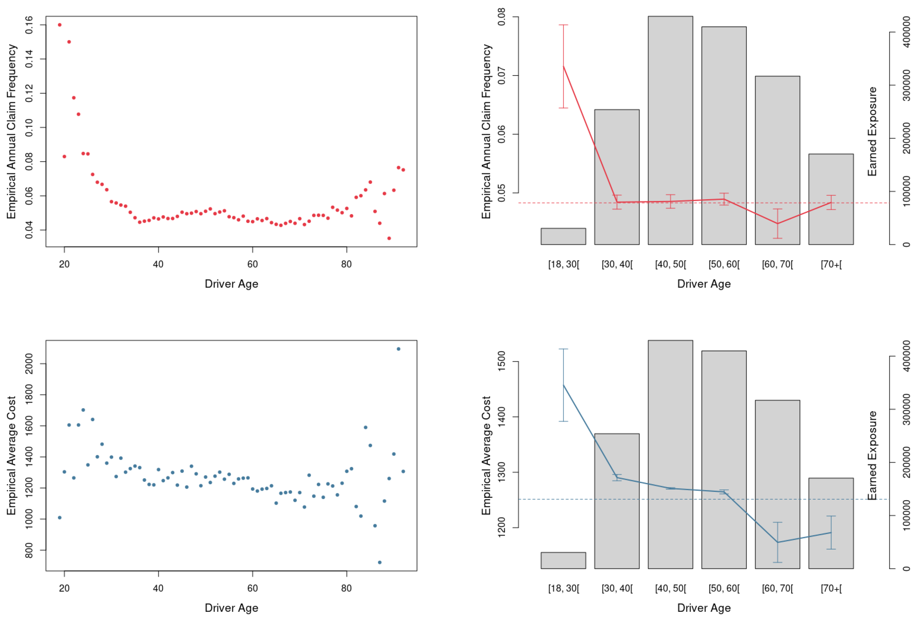
| Driver Age | 0–17, 18 to 85 (individually), 85+, unknown | Age of the usual driver |
| Cover Capital (Euro) | CapMin, CapMax | CapMax if the policy has the optional 59M TPL capital, or CapMin otherwise |
| NBexe (New Business) | RN, NB, FNB RN (renewal), NB (New Business), FNB (fake new business) | |
| Own Damage Cover | Yes, No | Yes (the policy includes own damage coverage) No (otherwise) |
| A. Claim frequency model | |||||
| # Fold () | # Trees | Shrinkage Factor | Interaction Depth | Bag Fraction | Poisson Deviance 1 |
| 1 | 37 | 0.10 | 2 | 0.95 | 0.2802844 |
| 2 | 64 | 0.10 | 2 | 0.95 | 0.2802088 |
| 3 | 642 | 0.01 | 2 | 0.80 | 0.2802078 |
| 4 | 116 | 0.10 | 1 | 0.95 | 0.2793700 |
| 5 | 239 | 0.05 | 2 | 0.95 | 0.2791459 |
| 6 | 47 | 0.10 | 4 | 0.95 | 0.2796919 |
| Average | 190 | 0.077 | 2 | 0.925 | – |
| B. Claim severity model | |||||
| # Fold () | # Trees | Shrinkage Factor | Interaction Depth | Bag Fraction | OOS Gamma Deviance 2 |
| 1 | 133 | 0.05 | 1 | 0.95 | 15.76648 |
| 2 | 125 | 0.05 | 1 | 0.95 | 15.76562 |
| 3 | 56 | 0.05 | 2 | 0.70 | 15.76658 |
| 4 | 33 | 0.1 | 1 | 0.80 | 15.76578 |
| 5 | 59 | 0.05 | 2 | 0.70 | 15.76709 |
| 6 | 75 | 0.1 | 1 | 0.95 | 15.76697 |
| Average | 80 | 0.067 | 1 | 0.925 | – |
| Sample | Total Poisson Deviance | Total Gamma Deviance | ||
|---|---|---|---|---|
| GLM | GBM | GLM | GBM | |
| Training (80%) | 432,456 | 428,621 | 8,787 | 10,545 |
| Testing (20%) | 107,914 | 106,773 | 2,162 | 2,624 |
| All (100%) | 540,406 | 535,685 | 10,954 | 13,209 |
| Variable | Level | Claim Frequency | Claim Severity | ||||
|---|---|---|---|---|---|---|---|
| Std. Error | p-Value | Std. Error | p-Value | ||||
| Intercept | – | −2.8334 | 0.0176 | ≈0 | 6.8804 | 0.01083 | ≈0 |
| Fuel | G2 | −0.1034 | 0.00958 | ≈0 | – | – | – |
| Vehicle Brand | G2 | 0.0421 | 0.01034 | 4.7 × | −0.0327 | 0.01268 | 9.9 × |
| Payment Instalments | G2 | 0.2138 | 0.00989 | ≈0 | – | – | – |
| G3 | 0.4288 | 0.01447 | ≈0 | – | – | – | |
| District | G2 | −0.3905 | 0.01142 | ≈0 | −0.0863 | 0.02079 | 3.3 × |
| G3 | −0.2743 | 0.01039 | ≈0 | 0.0909 | 0.02463 | 2.2 × | |
| Driver Age | G1 | −0.1597 | 0.02357 | ≈0 | 0.0736 | 0.03396 | 3 × |
| G3 | 0.02032 | 0.02122 | ≈0 | – | – | – | |
| G4 | 0.5415 | 0.03041 | ≈0 | −0.0938 | 0.01644 | 1.14 × | |
| G5 | 0.1544 | 0.01219 | ≈0 | −0.0938 | 0.01644 | 1.14 × | |
| G6 | 0.2874 | 0.02380 | ≈0 | −0.0938 | 0.01644 | 1.14 × | |
| Years Driving | G1 | 0.9770 | 0.06352 | ≈0 | – | – | – |
| G2 | 0.6739 | 0.05099 | ≈0 | – | – | – | |
| G3 | 0.4385 | 0.03676 | ≈0 | – | – | – | |
| G4 | 0.2549 | 0.02842 | ≈0 | – | – | – | |
| G5 | 0.1419 | 0.01926 | ≈0 | – | – | – | |
| G7 | −0.0608 | 0.01373 | 9.5 × | – | – | – | |
| G8 | −0.1289 | 0.01644 | ≈0 | – | – | – | |
| Vehicle Age | G2 | −0.1607 | 0.01454 | ≈0 | – | – | – |
| Horse Power | G2 | −0.1625 | 0.04331 | ≈0 | – | – | – |
| Time on Book | G2 | −0.1032 | 0.01533 | ≈0 | – | – | – |
| G3 | −0.1806 | 0.01498 | ≈0 | – | – | – | |
| G4 | −0.2969 | 0.01517 | ≈0 | – | – | – | |
| G5 | −0.3910 | 0.01671 | ≈0 | – | – | – | |
| G6 | −0.5036 | 0.03379 | ≈0 | – | – | – | |
| Frequency | Severity | ||
|---|---|---|---|
| GLM | GBM | GLM | GBM |
| Age of the Driver | Age of the Driver | Age of the Driver | Age of the Driver |
| Years of Driving | – | – | Years of Driving |
| District | District | District | District |
| – | Client Time on Book | – | – |
| Policy Time on Book | Policy Time on Book | – | – |
| Payment Instalments | Payment Instalments | Payment Instalments | Payment Instalments |
| – | Bonus–Malus | – | – |
| Brand | Brand | Brand | Brand |
| Vehicle Age | Vehicle Age | – | – |
| Horse Power | Horse Power | – | – |
| Fuel | – | – | – |
| – | – | – | Vehicle Weight |
| Variables | H-Statistic |
|---|---|
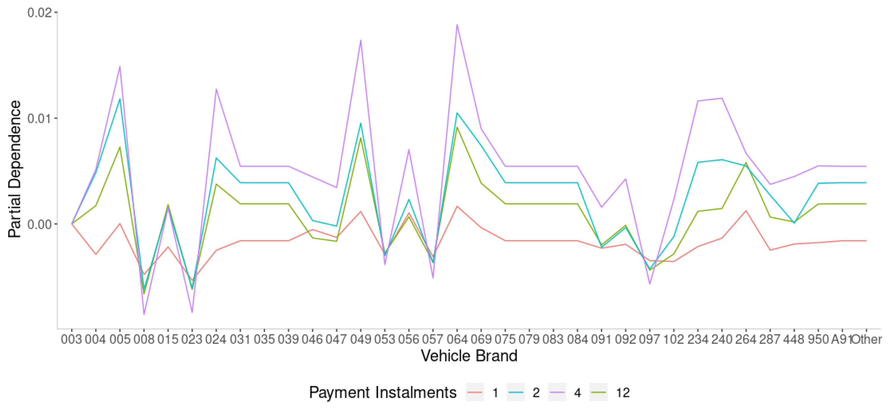
| (Payment Instalments, Vehicle Brand) | 0.2255 |
| (District, Policy seniority) | 0.2004 |
| (Client seniority, Vehicle Age) | 0.1560 |
| (Bonus–Malus, Payment Instalments) | 0.1424 |
| (Payment Instalments, Policy seniority) | 0.1355 |
| (District, Vehicle Brand) | 0.1147 |
| (Bonus–Malus, District) | 0.1038 |
| (District, Payment Instalments) | 0.0868 |
| (Bonus–Malus, Vehicle Brand) | 0.0867 |
| (District, Vehicle Age) | 0.0695 |
Disclaimer/Publisher’s Note: The statements, opinions and data contained in all publications are solely those of the individual author(s) and contributor(s) and not of MDPI and/or the editor(s). MDPI and/or the editor(s) disclaim responsibility for any injury to people or property resulting from any ideas, methods, instructions or products referred to in the content. |
© 2023 by the authors. Licensee MDPI, Basel, Switzerland. This article is an open access article distributed under the terms and conditions of the Creative Commons Attribution (CC BY) license (https://creativecommons.org/licenses/by/4.0/).
Share and Cite
Clemente, C.; Guerreiro, G.R.; Bravo, J.M. Modelling Motor Insurance Claim Frequency and Severity Using Gradient Boosting. Risks 2023, 11, 163. https://doi.org/10.3390/risks11090163
Clemente C, Guerreiro GR, Bravo JM. Modelling Motor Insurance Claim Frequency and Severity Using Gradient Boosting. Risks. 2023; 11(9):163. https://doi.org/10.3390/risks11090163
Chicago/Turabian StyleClemente, Carina, Gracinda R. Guerreiro, and Jorge M. Bravo. 2023. "Modelling Motor Insurance Claim Frequency and Severity Using Gradient Boosting" Risks 11, no. 9: 163. https://doi.org/10.3390/risks11090163
APA StyleClemente, C., Guerreiro, G. R., & Bravo, J. M. (2023). Modelling Motor Insurance Claim Frequency and Severity Using Gradient Boosting. Risks, 11(9), 163. https://doi.org/10.3390/risks11090163