Invariance of the Mathematical Expectation of a Random Quantity and Its Consequences

Abstract

Possibility and probability are the two aspects of uncertainty, where uncertainty represents the ignorance of a given individual. The notion of alternative (or event) belongs to the domain of possibility. An event is intrinsically subdivisible and a quadratic metric, whose value is intrinsic or invariant, is used to study it. By subdividing the notion of alternative, a joint (bivariate) distribution of mass appears. The mathematical expectation of X is proved to be invariant using joint distributions of mass. The same is true for $X_{12}$ and $X_{12\dots m}$. This paper describes the notion of $\alpha$-product, which refers to joint distributions of mass, as a way to connect the concept of probability with multilinear matters that can be treated through statistical inference. This multilinear approach is a meaningful innovation with regard to the current literature. Linear spaces over $\mathbb{R}$ with a different dimension can be used as elements of probability spaces. In this study, a more general expression for a measure of variability referred to a single random quantity is obtained. This multilinear measure is obtained using different joint distributions of mass, which are all considered together.

1. Introduction

Possibility and probability are the two aspects of uncertainty, where uncertainty represents the ignorance of a given individual (Capotorti et al. 2014). Possibility means that one is interested in establishing a given set of alternatives, where each alternative contained in this set is an event (Egidi et al. 2022). An event is not a repeatable fact whose meaning is collective. An event is not even a measurable set according to measure theory. In this paper, an event is a single case, whose meaning is atomistic (de Finetti 1982b). Possibility obeys the rules of ordinary logic or two-valued logic. Probability is distributed over a given set of alternatives (Fortini et al. 2018). It obeys the rules of the logic of prevision (Berti et al. 2020), which is many-valued logic. In this paper, ordinary logic is connected with linear spaces over $\mathbb{R}$. Moreover, the logic of prevision is shown to be connected with linear spaces over $\mathbb{R}$. The linear spaces over $\mathbb{R}$ treated in this paper are endowed with a quadratic metric, which is used to obtain indices of a statistical nature related to random quantities. Bounded and continuous random quantities, whose possible alternatives belong to a closed interval, can be estimated via discrete random quantities identifying a finite partition of elements. The same is true with respect to bounded random quantities containing a countable infinity of possible alternatives. In this study, the author was therefore interested in evaluating the probability over those incompatible and exhaustive elements that identify the possible alternatives for a discrete random quantity (Gilio and Sanfilippo 2014). Finitely additive probabilities are chosen with respect to all the different elements of the partition into account. Everything is known about probability and its formal properties, but, several times, researchers have not been at all concerned with defining it. In this paper, the notion of probability is shown to be an appropriate tool and valuable guide for estimating and choosing under uncertainty and riskiness, so it cannot be a first principle, unlike point and line in geometry. Probability is not something objective, substituting expectations and sensations associated with a given individual. The unique probability existing in all the cases depends on psychological expectations and sensations (Viscusi and Evans 2006). A subjective opinion is a reasonable object of serious study. For this reason, the methodological rigour associated with the theory of decision making based on subjective probabilities cannot be denied (Angelini and Maturo 2022a). It is necessary to believe that what is contained in the two paradigmatic collections “Studies in subjective probability”, edited by Kyburg and Smokler, must still be taken into account (Cassese et al. 2020). To believe that what has been said by these two collections and numerous papers in accordance with them is negligible, as several scholars dealing with uncertainty and riskiness tend to think nowadays, is not useful for current quantitative research in economics and finance.

Study Objectives

In Section 2, mathematical aspects related to the space of alternatives are treated. The space of possible alternatives for a given individual is embedded in $E^n$, where $E^n$ is an n-dimensional Euclidean space. The latter is generated by n linearly independent basis vectors. A possible event or alternative is a possible value for a random quantity. It is preferable to speak about random quantity instead of random variable. This is because it is necessary to think of the numerical interpretation of single events. This interpretation is vectorial whenever one refers to a finite partition of alternatives. Section 3 focuses on financial assets. They are random goods. Their conceptual and mathematical characteristics are handled. Financial assets are studied under uncertainty and riskiness outside the budget set of a given decision maker whenever the structure of the expected utility function describing an individual’s specific attitude toward risk is taken into account. Section 4 shows why events are intrinsically subdivisible. Their subdivision is pursued as soon as it is sufficient for obtaining a joint (bivariate) distribution of mass. A more general expression for a measure of variability, referring to a single random quantity, is obtained by subdividing the notion of event. In Section 5, the mathematical expectation of X is proved to be invariant. Preliminary results to the proof of Proposition 1 are provided in its subsections. By subdividing the notion of alternative, it is possible to prove that the mathematical expectation of $X_{12}$ and $X_{12\dots m}$ is invariant too. The mathematical expectation of X, $X_{12}$, and $X_{12\dots m}$ is always obtained inside linear spaces over $\mathbb{R}$ provided with a quadratic metric. An appropriate dimension of each linear space over $\mathbb{R}$ is taken into account. It is known that the notion of exchangeability referring to events is a way to connect the concept of subjective probability with the classical course of action of statistical inference. This paper shows that the notion of $\alpha$-product, referring to bivariate distributions of mass, is a way to connect the concept of subjective probability with multilinear matters that can be treated using statistical inference. The $\alpha$-product between two n-dimensional vectors, where the latter represent the possible values for two marginal random quantities, identifies the distance between two marginal distributions of mass. Finally, Section 6 provides conclusions and future perspectives.

2. Single Events Studied in the Space of Alternatives

2.1. Preliminaries

Let $x_1,x_2,\dots ,x_n$ be ordered real variables. All the n-tuples of real numbers being taken by such variables identify a set. Each n-tuple is a point in the real n-space denoted by ${\mathbb{R}}^n$. The real numbers of each n-tuple are the coordinates of a point. Let

$$P_j=P(x_{1j},x_{2j},\dots ,x_{nj})$$

(1)

be a point of ${\mathbb{R}}^n$, whereas the point denoted by

$$O=O(0,0,\dots ,0)$$

(2)

is the origin of ${\mathbb{R}}^n$. If the rank of the matrix given by

$$\parallel P_1,P_2,\dots ,P_n\parallel$$

(3)

is equal to n, then the dimension of ${\mathbb{R}}^n$ is equal to n. A located vector of $E^n$ at its origin is defined as a pair of points written as $\overrightarrow{O{P}_j}$. $\overrightarrow{O{P}_j}$ is also denoted by ${\mathbf{x}}_{\left(j\right)}$ or ${\mathbf{x}}_j$, where the n real numbers expressed by $x_{i\left(j\right)}$, $i=1,2,\dots ,n$ are the components of ${\mathbf{x}}_j$. The dimension of $E^n$ is equal to n. $E^n$ is a closed structure with respect to two binary operations (see von Neumann 1936 for another closed structure related to $E^n$). Thus, it is endowed with a component-wise addition denoted by

$$\mathbf{x}+\mathbf{y}=\{x_1+y_1,x_2+y_2,\dots ,x_n+y_n\}.$$

(4)

Moreover, it is endowed with a component-wise scalar multiplication denoted by

$$\alpha \mathbf{x}=\{\alpha x_1,\alpha x_2,\dots ,\alpha x_n\},$$

(5)

where $\alpha$ is any real number. A point of ${\mathbb{R}}^n$ is a vector of $E^n$. The same ordered n-tuple of real numbers identifies them. Suppose that the coordinates of (1) are pairwise orthogonal. Since the same hypothesis holds for any $P\in {\mathbb{R}}^n$, the n real variables denoted by $x_1,x_2,\dots ,x_n$ identify a Cartesian coordinate system for ${\mathbb{R}}^n$. The structure of $E^n$ is of a Euclidean nature, so it is possible to use the Pythagorean theorem in order to determine the distance of P from O. One writes

$${\displaystyle {}_{}^2}d{\displaystyle {(O,P)}_{}^{}}=\sqrt{{\displaystyle \sum _{i=1}^n}{\displaystyle x_i^2}}.$$

(6)

With respect to $E^n$, this distance identifies the length of $\mathbf{x}$ denoted by $\parallel \mathbf{x}\parallel$.

Let $P_j$ and $P_h$ be two points belonging to ${\mathbb{R}}^n$, whose coordinates are pairwise orthogonal. A located vector denoted by $\overrightarrow{O{P}_j}$ corresponds to $P_j$. It is visualized as an arrow between O and $P_j$. O is called its beginning point, and $P_j$ is its endpoint. The located vector under consideration is denoted as ${\mathbf{x}}_j\in E^n$. Similarly, the located vector denoted with $\overrightarrow{O{P}_h}$ corresponds to $P_h$. It is visualized as an arrow between O and $P_h$. O is called its beginning point, and $P_h$ is its endpoint. The located vector is denoted by ${\mathbf{x}}_h\in E^n$. $P_j$ and $P_h$ also characterize $\overrightarrow{P_j{P}_h}$; hence, ${\mathbf{x}}_h-{\mathbf{x}}_j$. With respect to ${\mathbb{R}}^n$, the square of the distance between $P_j$ and $P_h$ is given by

$${}^2{d}^2(P_j,P_h)={\displaystyle \sum _{i=1}^n}{(x_{i\left(j\right)}-x_{i\left(h\right)})}^2={\displaystyle \sum _{i=1}^n}{\displaystyle x_{i\left(j\right)}^2}+{\displaystyle \sum _{i=1}^n}{\displaystyle x_{i\left(h\right)}^2}-2{\displaystyle \sum _{i=1}^n}{x}_{i\left(j\right)}{x}_{i\left(h\right)}.$$

(7)

With respect to $E^n$, the norm of ${\mathbf{x}}_h-{\mathbf{x}}_j$ is given by

$$\parallel {\mathbf{x}}_h-{\mathbf{x}}_j{\parallel }^2=\parallel {\mathbf{x}}_h{\parallel }^2+{\parallel {\mathbf{x}}_j\parallel }^2-2⟨{\mathbf{x}}_h,{\mathbf{x}}_j⟩,$$

(8)

where $⟨{\mathbf{x}}_h,{\mathbf{x}}_j⟩$ is called the scalar or inner product between ${\mathbf{x}}_h$ and ${\mathbf{x}}_j$. If $⟨{\mathbf{x}}_h,{\mathbf{x}}_j⟩=0$, then the two vectors are orthogonal. Given $\alpha \in \mathbb{R}$, the function expressed by $f\left(\alpha \right)=\parallel {\mathbf{x}}_h-\alpha {\mathbf{x}}_j{\parallel }^2$ is such that it is $f\left(\alpha \right)\ge 0$. The inequalities denoted by

$$|⟨{\mathbf{x}}_h,{\mathbf{x}}_j⟩|\le \parallel {\mathbf{x}}_h\parallel \parallel {\mathbf{x}}_j\parallel ,$$

(9)

and

$$\parallel {\mathbf{x}}_h+{\mathbf{x}}_j\parallel \le \parallel {\mathbf{x}}_h\parallel +\parallel {\mathbf{x}}_j\parallel$$

(10)

can therefore be written. The former is called the Schwarz inequality, whereas the latter is called the triangle inequality. The metric structure of $E^n$ is now complete. From (9), it follows that

$$\left|\frac{⟨{\mathbf{x}}_h,{\mathbf{x}}_j⟩}{\parallel {\mathbf{x}}_h\parallel \parallel {\mathbf{x}}_j\parallel }\right|\le 1,$$

(11)

so there exists one and only one angle denoted by $\Theta$, $0\le \Theta \le \pi$, such that

$$cos\Theta =\frac{⟨{\mathbf{x}}_h,{\mathbf{x}}_j⟩}{\parallel {\mathbf{x}}_h\parallel \parallel {\mathbf{x}}_j\parallel }.$$

(12)

The angle between ${\mathbf{x}}_h$ and ${\mathbf{x}}_j$ is expressed by $\Theta$.

Since the dimension of $E^n$ is equal to n, there are at most n linearly independent vectors. Given n vectors denoted by ${\mathbf{e}}_i$, $i=1,2,\dots ,n$, if the following expression

$${\lambda }^1{\mathbf{e}}_1+{\lambda }^2{\mathbf{e}}_2+\dots +{\lambda }^n{\mathbf{e}}_n={\lambda }^i{\mathbf{e}}_i=\mathbf{0}$$

(13)

implies that ${\lambda }^i=0$ for every i, with $i=1,2,\dots ,n$, then the n vectors denoted by ${\mathbf{e}}_1,{\mathbf{e}}_2,\dots ,{\mathbf{e}}_n$ are linearly independent. They form a basis of $E^n$ denoted by

$$B_n=\left\{{\mathbf{e}}_i|i\in I_n=\{1,2,\dots ,n\}\right\}.$$

(14)

The zero vector is expressed by $\mathbf{0}=\mathbf{x}+(-\mathbf{x})$ for any $\mathbf{x}\in E^n$. The $n+1$ vectors denoted by ${\mathbf{e}}_1,{\mathbf{e}}_2,\dots ,{\mathbf{e}}_n,\mathbf{x}$ are linearly dependent, so, in the following linear combination given by

$$x^i{\mathbf{e}}_i+(-\mathbf{x})=\mathbf{0},$$

(15)

the coefficients expressed by $x^i$ are not all equal to 0. This means that, using the Einstein summation notation, one has

$$\mathbf{x}=x^i{\mathbf{e}}_i,$$

(16)

where $x^i$ are the contravariant components of $\mathbf{x}$ with respect to $B_n$. A fundamental result is the following. With respect to $B_n$, suppose that $\mathbf{x}$ can be represented by

$$\mathbf{x}=y^i{\mathbf{e}}_i.$$

(17)

The two sides of the following expression

$$\mathbf{0}=(x^i-y^i){\mathbf{e}}_i$$

(18)

are obtained from the left-hand side of (16) minus the left-hand side of (17) together with the right-hand side of (16) minus the right-hand side of (17). Nevertheless, ${\mathbf{e}}_1,\dots ,{\mathbf{e}}_n$ are linearly independent, so $x^i=y^i$ for every i, with $i=1,2,\dots ,n$. The conclusion is therefore as follows:

Remark 1.

With respect to a basis of $E^n$ denoted by $B_n$, every vector of $E^n$ is uniquely expressed by one and only one set of contravariant components.

It is always possible to establish an orthonormal basis of $E^n$ using the Gram-Schmidt process. If ${\displaystyle B_n^{\prime }}$ is an orthonormal basis of $E^n$, then one writes

$$⟨{\mathbf{e}}_i,{\mathbf{e}}_j⟩={\delta }_{ij},$$

(19)

where ${\delta }_{ij}$ is the Kronecker delta. The Kronecker delta is also called the metric tensor. If $\mathbf{x}=x^i{\mathbf{e}}_i$, with ${\mathbf{e}}_i\in {\displaystyle B_n^{\prime }}$, $i=1,2,\dots ,n$, then its Euclidean norm is given by

$${\parallel \mathbf{x}\parallel }^2=⟨\mathbf{x},\mathbf{x}⟩=⟨x^i{\mathbf{e}}_i,x^j{\mathbf{e}}_j⟩=x^i{x}^j{\delta }_{ij}={\displaystyle \sum _{i=1}^n}{\left(x^i\right)}^2.$$

(20)

The contravariant components of a vector are geometrically its projections by parallelism onto the basis vectors. Conversely, the covariant components of a vector are, geometrically, its orthogonal projections onto the basis vectors. Let $\mathbf{x}$ be a vector. Let $B_n=\left\{{\mathbf{e}}_i\right\}$ be a basis of $E^n$. Without loss of generality, suppose that all vectors of $B_n$ have a norm equal to 1. Hence, the ith covariant component of $\mathbf{x}$ is given by

$$x_i=\frac{⟨\mathbf{x},{\mathbf{e}}_i⟩}{\parallel {\mathbf{e}}_i{\parallel }^2}=⟨\mathbf{x},{\mathbf{e}}_i⟩=⟨x^j{\mathbf{e}}_j,{\mathbf{e}}_i⟩=x^j⟨{\mathbf{e}}_j,{\mathbf{e}}_i⟩=x^j{g}_{ji},$$

(21)

where $g_{ji}$ is the metric tensor. It is not usually necessary to distinguish the metric tensor from its symmetric components. The number of its distinct and symmetric components is

$$\frac{n(n+1)}{2}.$$

(22)

This is because such a number coincides with a 2-combination with repetitions from a set of size n. It is possible to note the following:

Remark 2.

The components of the metric tensor coincide with the Kronecker delta whenever an orthonormal basis of $E^n$ is used. Whenever linear spaces over $\mathbb{R}$ are of a Euclidean nature, the contravariant and covariant components of a same vector are given by the same numbers.

What was introduced by Ricci and Levi-Civita is used in this paper, so the contravariant components of a vector are denoted by upper indices, whereas the covariant ones are denoted by lower indices.

2.2. From Propositions (Logical Entities) to Real Numbers and Vice Versa

The space of alternatives contains what is objectively possible. In this paper, what is objectively possible is studied together with what is subjectively probable. The structure is mathematically the same. The space of alternatives is a linear space over $\mathbb{R}$ of a Euclidean nature. Possibility never depends on a subjective opinion (Coletti et al. 2016). Conversely, probability always depends on a subjective opinion. If X is a random quantity, then a linear combination of n incompatible and exhaustive events denoted by $E_1,E_2,\dots ,E_n$ is written as

$$X=x^1|E_1|+x^2|E_2|+\dots +x^n|E_n|,$$

(23)

where $I\left(X\right)=\{x^1,x^2,\dots ,x^n\}$ is the set of possible values for X. $|E_i|$, $i=1,2,\dots ,n$, is the indicator of $E_i$. Its values are 1 or 0 when $E_i$ is true or false, respectively. $E_i$ is true or false whenever uncertainty ceases. The elements of $I\left(X\right)=\{x^1,x^2,\dots ,x^n\}$, where one can observe $x^1<x^2<\dots <x^n$, are the contravariant components of a vector of $E^n$ denoted by

$$\mathbf{x}=(x^1,x^2,\dots ,x^n).$$

(24)

If X is a vector of $E^n$, then it is possible to write

$$X=x^1|E_1|{\mathbf{e}}_1+x^2|E_2|{\mathbf{e}}_2+\dots +x^n|E_n|{\mathbf{e}}_n,$$

(25)

where ${\displaystyle B_n^{\prime }}=\left\{{\mathbf{e}}_i\right\}$ is an orthonormal basis of $E^n$. With respect to ${\displaystyle B_n^{\prime }}$, one writes

$$\mathbf{x}=x^1{\mathbf{e}}_1+x^2{\mathbf{e}}_2+\dots +x^n{\mathbf{e}}_n=x^i{\mathbf{e}}_i.$$

(26)

The covariant components of a vector of $E^n$ denoted by

$$\mathbf{p}=(p_1,p_2,\dots ,p_n)$$

(27)

represent n masses associated with n possible values for X. In the first phase, each mass can be found between 0 and 1, endpoints included. The mathematical expectation of X is given by the following scalar or inner product

$$\mathbf{P}\left(X\right)=x^1{p}_1+x^2{p}_2+\dots +x^n{p}_n=x^i{p}_i,$$

(28)

where $x^1\le \mathbf{P}\left(X\right)\le x^n$ (Berti et al. 2001). Even though contravariant and covariant components are used, $\mathbf{x}$ and $\mathbf{p}$ belong to the same Euclidean space. This means that it is also possible to use covariant components of $\mathbf{x}$ together with contravariant ones of $\mathbf{p}$. Nothing changes. The two vectors $\mathbf{x}$ and $\mathbf{p}$ express the two aspects of uncertainty, which are studied inside $E^n$. An attribute can be transformed into a number. A number can be transformed into a proposition containing an attribute. This proposition is either true or false whenever uncertainty ceases. The possible values for X are real numbers. They can be related to a random vector given by

$$\left(\begin{array}{c}|E_1|\\ |E_2|\\ ⋮\\ |E_n|\end{array}\right)$$

(29)

identifying a finite partition of alternatives, where $E_1$ is an unequivocally established proposition containing $x^1$ as an attribute, …, $E_n$ is an unequivocally established proposition containing $x^n$ as an attribute. One writes

$$X=x^1\left(\begin{array}{c}|E_1|\\ |E_2|\\ ⋮\\ |E_n|\end{array}\right)+x^2\left(\begin{array}{c}|E_1|\\ |E_2|\\ ⋮\\ |E_n|\end{array}\right)+\dots +x^n\left(\begin{array}{c}|E_1|\\ |E_2|\\ ⋮\\ |E_n|\end{array}\right),$$

(30)

so n random vectors expressed in the form given by (29) are considered in $E^n$. Within this context, the term “random” means that a given element is not known by an individual and consequently it is uncertain or possible for him or her, but well determined in itself (de Finetti 1982a). If $Y=|E_1|+|E_2|+\dots +|E_n|$ is the number of successes, then an arithmetic operation expressed by the addition is used in connection with events. It is also possible to apply logical or Boolean operations to real numbers. In the field of real numbers, it is possible to define

$$x\vee y=max(x,y),$$

(31)

$$x\wedge y=min(x,y),$$

(32)

and

$$\tilde{x}=1-x,$$

(33)

for any x and y that are real numbers. If one writes $\mathbf{P}\left(\tilde{E}\right)=\mathbf{P}(1-E)=1-\mathbf{P}\left(E\right)$, where $\tilde{E}=1-E$ and E are events studied together with their probabilities denoted by $\mathbf{P}$, then a logical or Boolean operation given by the negation is treated together with an arithmetic one expressed by the subtraction. After remarking on a unification between events and numbers, a unification between logical or Boolean operations and arithmetic operations is also used. Logical product, logical sum, and negation are not applicable to 0 and 1 only, but they are applicable to all real numbers.

3. Marginal and Bivariate Random Quantities: Conceptual and Mathematical Aspects

In this paper, a random quantity X is a financial asset. It is firstly studied under conditions of uncertainty. X is then a random good. Its expected return has to be estimated by a given decision maker based on returns that have been observed by him or her in the past. X is a mathematical function such that its image is the set of those real numbers assigned by X to a sample space denoted by $\Omega$. The latter is a finite set. Suppose that the possible values for X belonging to $I\left(X\right)=\Omega$ are all nonnegative, so one writes $X\ge 0$. This means that $\inf I\left(X\right)\ge 0$. In this paper, X is a bounded random good, so $\sup I\left(X\right)<+\infty$. Since it is always possible to write

$$X=X_1-X_2,$$

(34)

where one has

$$X_1=0\vee X,$$

(35)

and

$$X_2=|0\wedge X|,$$

(36)

X is a random quantity that is certainly nonnegative. The set of the coherent previsions of (34) is uncountable. This set is a closed line segment. If ${}_{1}X$ and ${}_{2}X$ are two financial assets, then the possible values for ${}_{1}X$ belonging to $I{(}_{1}X)$ and the possible ones for ${}_{2}X$ belonging to $I{(}_{2}X)$ are all nonnegative. Two perpendicular straight lines are considered. ${}_{1}X$ and ${}_{2}X$ are linearly independent. In this paper, ${}_{1}X$ and ${}_{2}X$ are two marginal random goods giving rise to a bivariate random good denoted by ${}_{1}X{}_{2}X$. Its possible values are expressed by $I{(}_{1}X)\times I{(}_{2}X)$. A subdivision of alternatives takes place in this way. The set of the coherent previsions of ${}_{1}X$, ${}_{2}X$, and ${}_{1}X{}_{2}X$ is a right triangle belonging to the first quadrant of the Cartesian plane, where the vertex of its right angle is given by the point $(0,0)$. Every point belonging to such a triangle is denoted by

$$\mathbf{P}{(}_{1}X{}_{2}X)\equiv \left(\mathbf{P}{(}_{1}X),\mathbf{P}{(}_{2}X)\right).$$

(37)

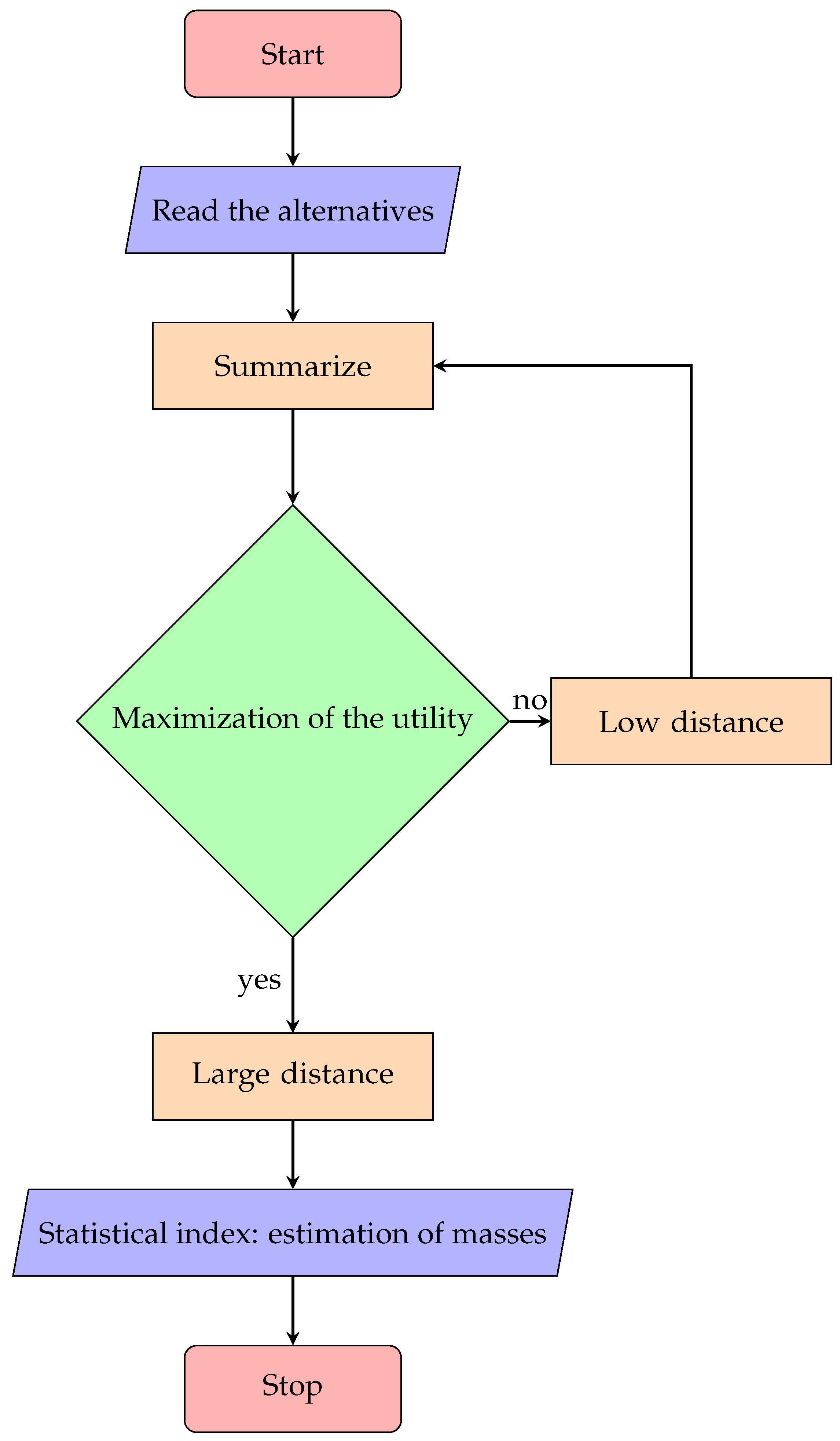
This triangle contains all fair estimations being made by a given individual. Given $\mathbf{P}{(}_{1}X)$ and $\mathbf{P}{(}_{2}X)$, it is possible to estimate the joint masses identifying $\mathbf{P}{(}_{1}X{}_{2}X)$ in such a way that one out of three values, $-1$, 0, and 1, associated with the correlation coefficient appears (it is usually $n\ge 10$). The correlation coefficient is equal to the covariance between ${}_{1}X$ and ${}_{2}X$ divided by the product of their standard deviations. With respect to the correlation coefficient, the possible values for ${}_{1}X$ and ${}_{2}X$ are deviations. Nevertheless, all masses underlying every point denoted by (37) do not change. If $-1$ is the value being taken by the correlation coefficient, then a given individual making a specific estimation of joint masses inside his or her budget set is a risk averter; if 0 is the value being taken, then an individual is risk neutral. If the correlation coefficient is equal to 1, then a given decision maker is a risk lover. The right triangle where all fair estimations appear is determined by a straight line, whose slope is negative. This line is a hyperplane. Its horizontal and vertical intercepts are established. From the ratio of these intercepts, it is possible to estimate the ratio of the prices of the two marginal random goods. The space where all fair estimations appear is endowed with boundary points. It is a subset of a linear space over $\mathbb{R}$. It is also possible to choose a specific point maximizing the subjective utility related to objects of decision maker estimation. This choice always depends on empirical aspects. Thus, it is essential to distinguish two phases: a formal and an empirical phase. The formal phase firstly establishes all fair estimations, whereas the empirical one secondly identifies a specific point belonging to the right triangle. The hyperplane never separates this specific point from all points expressing possible alternatives. In other words, the hyperplane under consideration leaves this specific point on the same side together with all points expressing possible alternatives. Applying the Pythagorean theorem to the points of the right triangle, it is possible to prove that the notion of ordinal utility is a distance. If ${}_{1}X$ and ${}_{2}X$ are the components of multiple goods of order 2 denoted by $X_{12}$, then $2^2=4$ bivariate distributions of mass have to be considered. This is because it is possible to exchange ${}_{1}X$ for $\mathbf{P}{(}_{1}X)$ and ${}_{2}X$ for $\mathbf{P}{(}_{2}X)$. This implies that it is necessary to exchange $X_{12}$ for $\mathbf{P}\left(X_{12}\right)$. The expected return on $X_{12}$, where $X_{12}$ is a portfolio containing two financial assets, is denoted by $\mathbf{P}\left(X_{12}\right)$. The latter index contains $2^2=4$ bivariate distributions of mass, which are all summarized. This result is innovative. By considering more than two marginal random goods, similar indices are obtained. What is observed inside the right triangle can be used to handle the notion of expected utility (cardinal utility) outside it. Hence, choice problems related to financial assets that are studied under uncertainty and riskiness outside the budget set of a given decision maker depend on the structure of the expected utility function describing an individual’s specific attitude toward risk. This expected utility function is treated inside a subset of a linear space over $\mathbb{R}$. The notion of cardinal utility is based on a distance too. It is of interest to take the following Figure 1 as a guide.

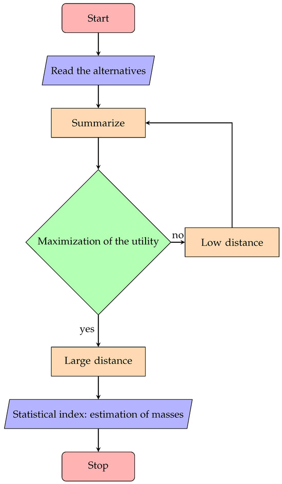
Figure 1. A flowchart representing an optimal decision making process.

4. A Marginal Random Quantity Studied as a Double Quantity: The Central Role of Bivariate Distributions of Mass

Given two sets of alternatives, where each of them is denoted by $\{a,b,c\}$, it is possible to study the Cartesian product given by $\{a,b,c\}\times \{a,b,c\}$. If such a product is handled, then $3^2=9$ elements appear. A subdivision of alternatives appears in this way. Given a marginal random quantity denoted by ${}_{1}X$, to study it as a double one denoted by $X_{12}$ means that four bivariate random quantities denoted by ${}_{1}X{}_{1}X$, ${}_{1}X{}_{2}X$, ${}_{2}X{}_{1}X$, and ${}_{2}X{}_{2}X$ are treated. One writes

$$X_{12}={\{}_{1}X,{}_{2}X\}.$$

(38)

The components of $X_{12}$ are ${}_{1}X$ and ${}_{2}X$. A multilinear approach is used. This approach is a meaningful innovation with respect to those in the current literature (Grechuk et al. 2012). This approach is useful for obtaining multilinear measures. Such measures can be used to study new types of relationships between variables. If a marginal random quantity has n values, then a bivariate random quantity has $n^2$ values (see Pompilj 1957 in connection with the notion of independence). One has

$$dim\left(E^n\right)=n,$$

(39)

so one observes

$$dim(E^n\otimes E^n)=n^2,$$

(40)

where $E^n\otimes E^n$ is a linear space over $\mathbb{R}$. From (25), it follows that

$${}_{1}X{}_{2}X={\displaystyle {}_{\left(1\right)}^{}}{\displaystyle x_{}^1}{\displaystyle {}_{\left(2\right)}^{}}{\displaystyle x_{}^1}|{\displaystyle {}_{\left(1\right)}^{}}{\displaystyle E_1^{}}||{\displaystyle {}_{\left(2\right)}^{}}{\displaystyle E_1^{}}|{\mathbf{e}}_1\otimes {\mathbf{e}}_1+\dots +{\displaystyle {}_{\left(1\right)}^{}}{\displaystyle x_{}^n}{\displaystyle {}_{\left(2\right)}^{}}{\displaystyle x_{}^n}|{\displaystyle {}_{\left(1\right)}^{}}{\displaystyle E_n^{}}||{\displaystyle {}_{\left(2\right)}^{}}{\displaystyle E_n^{}}|{\mathbf{e}}_n\otimes {\mathbf{e}}_n.$$

(41)

Two conditions hold if one wants to represent ${}_{1}X$ as $X_{12}$. The first condition is the following:

$$\mathbf{P}{(}_{1}X)={\displaystyle \sum _{i_1=1}^n}{\displaystyle {}_{\left(1\right)}^{}}{\displaystyle x_{}^{i_1}}p{}_{i_1}.$$

(42)

The following expression

$$p=p_{i_1{i}_2}$$

(43)

is an affine tensor of order 2. Its covariant components express all joint masses. The following relationship

$${\displaystyle \sum _{i_1=1}^n}{\displaystyle {}_{\left(1\right)}^{}}{\displaystyle x_{}^{i_1}}p{}_{i_1}={\displaystyle \sum _{i_1,i_2=1}^n}{\displaystyle {}_{\left(1\right)}^{}}{\displaystyle x_{}^{i_1}}p{}_{i_1{i}_2}$$

(44)

holds if (43) is used. The two sides of (44) are equal if and only if

$${\displaystyle \sum _{i_1=1}^n}p{}_{i_1}={\displaystyle \sum _{i_1,i_2=1}^n}p{}_{i_1{i}_2}.$$

(45)

One finally writes

$${\displaystyle \sum _{i_1=1}^n}p{}_{i_1}={\displaystyle \sum _{i_1,i_2=1}^n}p{}_{i_1{i}_2}=1,$$

(46)

so ${}_{1}X$ and ${}_{1}X{}_{2}X$ are two finite partitions of incompatible and exhaustive alternatives. The second condition is as follows: ${}_{1}X$ and ${}_{1}X{}_{2}X$ must have the same mean value (Nunke and Savage 1952). One writes

$${\displaystyle \sum _{i_1,i_2=1}^n}{\displaystyle {}_{\left(1\right)}^{}}{\displaystyle x_{}^{i_1}}{\displaystyle {}_{\left(2\right)}^{}}{\displaystyle x_{}^{i_2}}p{}_{i_1{i}_2}={\displaystyle \sum _{i_1,i_2=1}^n}{\displaystyle {}_{\left(1\right)}^{}}{\displaystyle x_{}^{i_1}}p{}_{i_1{i}_2},$$

(47)

so the two sides of (47) are equal if and only if

$${\displaystyle {}_{\left(2\right)}^{}}{\displaystyle x_{}^{i_2}}=1,\forall i_2\in I_n.$$

(48)

Hence, it is possible to note the following:

Remark 3.

Let $B_n=\left\{{\mathbf{e}}_i\right\}$, $i=1,\dots ,n$, be an orthonormal basis of $E^n$. The possible values for the other random quantity, such that ${}_{1}X$ is studied as $X_{12}$, form the set denoted by

$$\left\{1^i\right\}.$$

(49)

The number of elements of (49) is equal to n. Such components depend on the basis of $E^n$ being arbitrarily chosen. From $B_n$ to ${\displaystyle B_n^{\prime }}=\left\{{\mathbf{e}}_{i^{\prime }}\right\}$, $i^{\prime }=1,\dots ,n$, one has

$$1^{i^{\prime }}={\displaystyle a_i^{i^{\prime }}}{1}^i={\displaystyle \sum _{i=1}^n}{\displaystyle a_i^{i^{\prime }}},$$

(50)

where $A=\left({\displaystyle a_i^{i^{\prime }}}\right)$ is an $n\times n$ matrix expressing a change of basis.

Remark 4.

The vector of $E^n$ with contravariant components forming the set expressed by

$$\{{\varphi }^1=1,{\varphi }^2=1,\dots ,{\varphi }^n=1\}$$

(51)

is denoted by $\mathit{\varphi }$.

A Measure of Variability Obtained Using a Multilinear Approach: A Numerical Example

A marginal distribution of mass of ${}_{1}X$ can coincide with a bivariate distribution of ${}_{1}X$ and ${}_{2}X=\mathit{\varphi }$. Nonparametric distributions of mass are used. For instance, Table 1 gives $\mathbf{P}{(}_{1}X)=\mathbf{P}{(}_{1}X{}_{2}X)=\mathbf{P}{(}_{2}X{}_{1}X)=5.2$. Since $\mathbf{P}{(}_{1}X{}_{1}X)=28$ and $\mathbf{P}{(}_{2}X{}_{2}X)=1$ are observed, the variance of ${}_{1}X$ is given by

$${\displaystyle {\sigma }_{{}_{1}X}^2}=\left|\begin{array}{cc}\mathbf{P}{(}_{1}X{}_{1}X)=28& \mathbf{P}{(}_{1}X{}_{2}X)=5.2\\ \mathbf{P}{(}_{2}X{}_{1}X)=5.2& \mathbf{P}{(}_{2}X{}_{2}X)=1\end{array}\right|=0.96.$$

(52)

The variance of ${}_{1}X$ is established as if ${}_{1}X$ coincides with $X_{12}={\{}_{1}X,\mathit{\varphi }\}$. A measure of variability, related to a single random quantity, is obtained using a multilinear approach. The notion of alternative is subjected to a subdivision, so four bivariate distributions are treated. A quadratic metric is used (Berkhouch et al. 2018; Gerstenberger and Vogel 2015).

Table 1. A univariate distribution transformed into a bivariate distribution.

	${}_2\mathit{X}=\mathit{\varphi }$	1	1	1	Sum
${}_1\mathit{X}$
0		0	0	0	0
4		0	0.4	0	0.4
6		0	0	0.6	0.6
Sum		0	0.4	0.6	1

5. Invariance of the Notion of Mathematical Expectation of a Random Quantity

5.1. Change of Basis

Let $B_n=\left\{{\mathbf{e}}_i\right\}$, $i=1,\dots ,n$, be an orthonormal basis of $E^n$. Let ${\displaystyle B_n^{\prime }}=\left\{{\mathbf{e}}_{j^{\prime }}\right\}$, $j^{\prime }=1,\dots ,n$, be another orthonormal basis of $E^n$. Each vector of ${\displaystyle B_n^{\prime }}$ can be expressed as a linear combination of the vectors of $B_n$, so one writes

$${\mathbf{e}}_{j^{\prime }}={\displaystyle A_{j^{\prime }}^i}{\mathbf{e}}_i.$$

(53)

If i varies, then the set given by $\left\{{\displaystyle A_{j^{\prime }}^i}\right\}$ identifies the n contravariant components of ${\mathbf{e}}_{j^{\prime }}$ with respect to the vectors of $B_n$. If $j^{\prime }$ varies together with i, then the set given by $\left\{{\displaystyle A_{j^{\prime }}^i}\right\}$ identifies $n\times n$ real numbers leading to the notion of square matrix of order n. If a basis of $E^n$ changes, then $\mathbf{x}\in E^n$ does not change. Conversely, its contravariant components change, so the following equalities appear

$$\mathbf{x}=x^i{\mathbf{e}}_i=x^{j^{\prime }}{\mathbf{e}}_{j^{\prime }}=x^{j^{\prime }}{\displaystyle A_{j^{\prime }}^i}{\mathbf{e}}_i.$$

(54)

From

$$x^i{\mathbf{e}}_i=x^{j^{\prime }}{\displaystyle A_{j^{\prime }}^i}{\mathbf{e}}_i,$$

(55)

where ${\mathbf{e}}_i$ is found in both sides of what one has just written, it follows that it is possible to obtain

$$x^i={\displaystyle A_{j^{\prime }}^i}{x}^{j^{\prime }}.$$

(56)

(56) gives how the contravariant components of $\mathbf{x}\in E^n$ change whenever one passes from ${\displaystyle B_n^{\prime }}$ to $B_n$. From

$$x^{j^{\prime }}{\mathbf{e}}_{j^{\prime }}=x^{j^{\prime }}{\displaystyle A_{j^{\prime }}^i}{\mathbf{e}}_i,$$

(57)

where $x^{j^{\prime }}$ is found in both sides of what one has just written, it follows that it is possible to obtain the expression given by (53). $A=\left\{{\displaystyle A_{j^{\prime }}^i}\right\}$ is an orthogonal matrix. The inverse of A is therefore equal to its transpose.

5.2. Invariant or Intrinsic Metric

If the expression given by (56) is considered, then the Euclidean norm of $\mathbf{x}\in E^n$ identified with (20) is invariant. This is because one writes

$${\displaystyle \sum _{i=1}^n}{\left(x^i\right)}^2={\displaystyle \sum _{i=1}^n}{\displaystyle A_{j^{\prime }}^i}{\displaystyle A_{h^{\prime }}^i}{x}^{j^{\prime }}{x}^{h^{\prime }}.$$

(58)

This happens because both $B_n$ and ${\displaystyle B_n^{\prime }}$ are considered. The set given by the following numbers

$$g_{j^{\prime }{h}^{\prime }}={\displaystyle \sum _{i=1}^n}{\displaystyle A_{j^{\prime }}^i}{\displaystyle A_{h^{\prime }}^i}=⟨{\mathbf{e}}_{j^{\prime }},{\mathbf{e}}_{h^{\prime }}⟩$$

(59)

identifies the components of the metric tensor, whose nature is symmetric. Accordingly, one writes

$$g_{j^{\prime }{h}^{\prime }}=g_{h^{\prime }{j}^{\prime }}.$$

(60)

5.3. Change-of-Basis Matrices

Let ${\displaystyle B_n^{\prime }}=\left\{{\mathbf{e}}_{j^{\prime }}\right\}$ and ${\displaystyle B_n^{″}}=\left\{{\mathbf{e}}_{h^{″}}\right\}$ be two orthonormal bases of $E^n$. Since one writes

$${\mathbf{e}}_{j^{\prime }}={\displaystyle B_{j^{\prime }}^{h^{″}}}{\mathbf{e}}_{h^{″}},$$

(61)

and

$${\mathbf{e}}_{h^{″}}={\displaystyle C_{h^{″}}^{i^{\prime }}}{\mathbf{e}}_{i^{\prime }},$$

(62)

the second expressions can be put into the first ones. This means that one has

$${\mathbf{e}}_{j^{\prime }}={\displaystyle B_{j^{\prime }}^{h^{″}}}{\displaystyle C_{h^{″}}^{i^{\prime }}}{\mathbf{e}}_{i^{\prime }}.$$

(63)

(63) can also be written in the following form

$${\mathbf{e}}_{i^{\prime }}{\displaystyle {\delta }_{j^{\prime }}^{i^{\prime }}}={\displaystyle B_{j^{\prime }}^{h^{″}}}{\displaystyle C_{h^{″}}^{i^{\prime }}}{\mathbf{e}}_{i^{\prime }},$$

(64)

so one has

$${\displaystyle {\delta }_{j^{\prime }}^{i^{\prime }}}={\displaystyle B_{j^{\prime }}^{h^{″}}}{\displaystyle C_{h^{″}}^{i^{\prime }}}.$$

(65)

It follows that $B=\left\{{\displaystyle B_{j^{\prime }}^{h^{″}}}\right\}$ is the inverse of $C=\left\{{\displaystyle C_{h^{″}}^{i^{\prime }}}\right\}$ and vice versa, where B and C are two square matrices of order n. Let $\mathbf{x}\in E^n$ be a vector. Its contravariant components identify a family of n incompatible and exhaustive alternatives. Such a vector can be expressed by

$$\mathbf{x}=x^{i^{\prime }}{\mathbf{e}}_{i^{\prime }}$$

(66)

with respect to the vectors of ${\displaystyle B_n^{\prime }}$. The same vector $\mathbf{x}\in E^n$ can be expressed by

$$\mathbf{x}=x^{h^{″}}{\mathbf{e}}_{h^{″}}$$

(67)

with respect to the vectors of ${\displaystyle B_n^{″}}$. If one passes from ${\displaystyle B_n^{″}}$ to ${\displaystyle B_n^{\prime }}$, then one has

$$x^{h^{″}}={\displaystyle C_{i^{\prime }}^{h^{″}}}{x}^{i^{\prime }}.$$

(68)

The vector $\mathbf{x}\in E^n$ is always the same. Only its contravariant components change whenever one passes from a basis of $E^n$ to the other one. One observes

$$\mathbf{x}=x^{i^{\prime }}{\mathbf{e}}_{i^{\prime }}=\left({\displaystyle C_{i^{\prime }}^{h^{″}}}{x}^{i^{\prime }}\right)\left({\displaystyle C_{h^{″}}^{j^{\prime }}}{\mathbf{e}}_{j^{\prime }}\right)=\left({\displaystyle C_{i^{\prime }}^{h^{″}}}{\displaystyle C_{h^{″}}^{j^{\prime }}}\right)\left(x^{i^{\prime }}{\mathbf{e}}_{j^{\prime }}\right)$$

(69)

because (68) and (62) are put into (67). Since

$${\displaystyle C_{i^{\prime }}^{h^{″}}}{\displaystyle C_{h^{″}}^{j^{\prime }}}={\displaystyle {\delta }_{i^{\prime }}^{j^{\prime }}},$$

(70)

the square matrix, whose generic element is given by ${\displaystyle C_{i^{\prime }}^{h^{″}}}$, is the inverse of the square matrix, whose generic element is expressed by ${\displaystyle C_{h^{″}}^{j^{\prime }}}$.

5.4. Invariant Scalar Product

With respect to ${\displaystyle B_n^{\prime }}$, the scalar or inner product between $\mathbf{x},\mathbf{y}\in E^n$ is denoted by ${⟨\mathbf{x},\mathbf{y}⟩}^{\prime }$. With respect to ${\displaystyle B_n^{″}}$, the scalar or inner product between the same vectors of $E^n$ is conversely denoted by ${⟨\mathbf{x},\mathbf{y}⟩}^{″}$. Thus, it is possible to prove the following:

Proposition 1.

The scalar or inner product between $\mathbf{x},\mathbf{y}\in E^n$ is invariant, so ${⟨\mathbf{x},\mathbf{y}⟩}^{\prime }={⟨\mathbf{x},\mathbf{y}⟩}^{″}$.

Proof. 

With respect to ${\displaystyle B_n^{\prime }}$, one has

$${⟨\mathbf{x},\mathbf{y}⟩}^{\prime }=⟨x^{i^{\prime }}{\mathbf{e}}_{i^{\prime }},y^{j^{\prime }}{\mathbf{e}}_{j^{\prime }}⟩=x^{i^{\prime }}{y}^{j^{\prime }}⟨{\mathbf{e}}_{i^{\prime }},{\mathbf{e}}_{j^{\prime }}⟩=x^{i^{\prime }}{y}^{j^{\prime }}{g}_{i^{\prime }{j}^{\prime }}.$$

(71)

Similarly, with respect to ${\displaystyle B_n^{″}}$, one writes

$${⟨\mathbf{x},\mathbf{y}⟩}^{″}=x^{i^{″}}{y}^{j^{″}}{g}_{i^{″}{j}^{″}}.$$

(72)

If one passes from ${\displaystyle B_n^{″}}$ to ${\displaystyle B_n^{\prime }}$, then the components of the metric tensor become

$$g_{i^{″}{j}^{″}}=⟨{\mathbf{e}}_{i^{″}},{\mathbf{e}}_{j^{″}}⟩=⟨{\displaystyle C_{i^{″}}^{h^{\prime }}}{\mathbf{e}}_{h^{\prime }},{\displaystyle C_{j^{″}}^{k^{\prime }}}{\mathbf{e}}_{k^{\prime }}⟩={\displaystyle C_{i^{″}}^{h^{\prime }}}{\displaystyle C_{j^{″}}^{k^{\prime }}}{g}_{h^{\prime }{k}^{\prime }}.$$

(73)

Since

$$\begin{array}{cc}\hfill {⟨\mathbf{x},\mathbf{y}⟩}^{″}& =\left({\displaystyle C_{r^{\prime }}^{i^{″}}}{x}^{r^{\prime }}\right)\left({\displaystyle C_{s^{\prime }}^{j^{″}}}{y}^{s^{\prime }}\right){\displaystyle C_{i^{″}}^{h^{\prime }}}{\displaystyle C_{j^{″}}^{k^{\prime }}}{g}_{h^{\prime }{k}^{\prime }}\hfill \\ & =\left({\displaystyle C_{r^{\prime }}^{i^{″}}}{\displaystyle C_{i^{″}}^{h^{\prime }}}\right)\left({\displaystyle C_{s^{\prime }}^{j^{″}}}{\displaystyle C_{j^{″}}^{k^{\prime }}}\right)x^{r^{\prime }}{y}^{s^{\prime }}{g}_{h^{\prime }{k}^{\prime }}\hfill \\ & ={\displaystyle {\delta }_{r^{\prime }}^{h^{\prime }}}{\displaystyle {\delta }_{s^{\prime }}^{k^{\prime }}}{x}^{r^{\prime }}{y}^{s^{\prime }}{g}_{h^{\prime }{k}^{\prime }}\hfill \\ & =x^{h^{\prime }}{y}^{k^{\prime }}{g}_{h^{\prime }{k}^{\prime }}\hfill \\ & ={⟨\mathbf{x},\mathbf{y}⟩}^{\prime },\hfill \end{array}$$

the equality given by

$${⟨\mathbf{x},\mathbf{y}⟩}^{″}={⟨\mathbf{x},\mathbf{y}⟩}^{\prime }$$

(74)

proves that the scalar or inner product between $\mathbf{x},\mathbf{y}\in E^n$ is invariant.  □

5.5. The Notion of $\alpha$-Product

A marginal random quantity denoted by X can always be expressed using a bivariate distribution of mass. The mathematical expectation of X denoted by $\mathbf{P}\left(X\right)$ is obtained by summarizing a bivariate distribution of mass through the notion of $\alpha$-product. The $\alpha$-product is a scalar or inner product. Its four formal properties are as follows: it is a commutative, associative, distributive, and orthogonal scalar or inner product. The mathematical expectation of $X_{12}={\{}_{1}X,{}_{2}X\}$ is denoted by $\mathbf{P}\left(X_{12}\right)$. One has

$$\mathbf{P}\left(X_{12}\right)=\left|\begin{array}{cc}\mathbf{P}{(}_{1}X{}_{1}X)& \mathbf{P}{(}_{1}X{}_{2}X)\\ \mathbf{P}{(}_{2}X{}_{1}X)& \mathbf{P}{(}_{2}X{}_{2}X)\end{array}\right|,$$

(75)

where $X_{12}$ is a double random quantity. Four $\alpha$-products are $\mathbf{P}{(}_{1}X{}_{1}X)$, $\mathbf{P}{(}_{1}X{}_{2}X)$, $\mathbf{P}{(}_{2}X{}_{1}X)$, and $\mathbf{P}{(}_{2}X{}_{2}X)$. Each of them is intrinsically of a two-dimensional nature. Each of them is then expressed using an ordered pair of real numbers. This is because each of them is a measure of a bilinear nature that is decomposed into two linear measures. $\mathbf{P}\left(X_{12}\right)$ is, conversely, a real number. It is the determinant of a square matrix of order 2. In general, the mathematical expectation of a multiple random quantity of order m denoted by

$$X_{12\dots m}={\{}_{1}X,{}_{2}X,\dots ,{}_{m}X\}$$

(76)

is expressed as $\mathbf{P}\left(X_{12\dots m}\right)$. One has

$$\mathbf{P}\left(X_{12\dots m}\right)=\left|\begin{array}{cccc}\mathbf{P}{(}_{1}X{}_{1}X)& \mathbf{P}{(}_{1}X{}_{2}X)& \dots & \mathbf{P}{(}_{1}X{}_{m}X)\\ \mathbf{P}{(}_{2}X{}_{1}X)& \mathbf{P}{(}_{2}X{}_{2}X)& \dots & \mathbf{P}{(}_{2}X{}_{m}X)\\ ⋮& ⋮& \ddots & ⋮\\ \mathbf{P}{(}_{m}X{}_{1}X)& \mathbf{P}{(}_{m}X{}_{2}X)& \dots & \mathbf{P}{(}_{m}X{}_{m}X)\end{array}\right|,$$

(77)

where $m^2$$\alpha$-products are used. (75) is the $\alpha$-norm of a particular tensor of order 2, whereas (77) is the $\alpha$-norm of a particular tensor of order m. In either case, bivariate distributions of mass are always used. How the notion of $\alpha$-product between ${\displaystyle {}_{\left(1\right)}^{}}{\displaystyle {\mathbf{x}}_{}^{}}$ and ${\displaystyle {}_{\left(2\right)}^{}}{\displaystyle {\mathbf{x}}_{}^{}}$, with ${\displaystyle {}_{\left(1\right)}^{}}{\displaystyle {\mathbf{x}}_{}^{}}$, ${\displaystyle {}_{\left(2\right)}^{}}{\displaystyle {\mathbf{x}}_{}^{}}\in E^n$, works is explained as follows:

Example 1.

Table 2 gives $\mathbf{P}{(}_{1}X{}_{2}X)=55.2$. The contravariant components of ${\displaystyle {}_{\left(2\right)}^{}}{\displaystyle {\mathbf{x}}_{}^{}}$ identify the following column vector

$$\left(\begin{array}{c}0\\ 6\\ 7\end{array}\right),$$

whereas its covariant components are given by

$$0·0+6·0+7·0=0,$$

$$0·0+6·0.2+7·0.3=3.3,$$

and

$$0·0+6·0.3+7·0.2=3.2.$$

It is then possible to observe

$$⟨\left(\begin{array}{c}0\\ 8\\ 9\end{array}\right),\left(\begin{array}{c}0\\ 3.3\\ 3.2\end{array}\right)⟩={⟨{\displaystyle {}_{\left(1\right)}^{}}{\displaystyle {\mathbf{x}}_{}^{}},{\displaystyle {}_{\left(2\right)}^{}}{\displaystyle {\mathbf{x}}_{}^{}}⟩}_{\alpha }=\mathbf{P}{(}_{1}X{}_{2}X)=55.2.$$

After calculating the covariant components of ${\displaystyle {}_{\left(1\right)}^{}}{\displaystyle {\mathbf{x}}_{}^{}}$ in a similar way, one writes

$$⟨\left(\begin{array}{c}0\\ 4.3\\ 4.2\end{array}\right),\left(\begin{array}{c}0\\ 6\\ 7\end{array}\right)⟩={⟨{\displaystyle {}_{\left(1\right)}^{}}{\displaystyle {\mathbf{x}}_{}^{}},{\displaystyle {}_{\left(2\right)}^{}}{\displaystyle {\mathbf{x}}_{}^{}}⟩}_{\alpha }=\mathbf{P}{(}_{1}X{}_{2}X)=55.2.$$

The notion of α-norm is as follows: Table 3 gives $\parallel {\displaystyle {}_{\left(1\right)}^{}}{\displaystyle {\mathbf{x}}_{}^{}}{\displaystyle {\parallel }_{\alpha }^2}=\mathbf{P}{(}_{1}X{}_{1}X)=72.5$, whereas Table 4 gives $\parallel {\displaystyle {}_{\left(2\right)}^{}}{\displaystyle {\mathbf{x}}_{}^{}}{\displaystyle {\parallel }_{\alpha }^2}=\mathbf{P}{(}_{2}X{}_{2}X)=42.5$. It follows that

$$\mathbf{P}\left(X_{12}\right)=\left|\begin{array}{cc}\mathbf{P}{(}_{1}X{}_{1}X)=72.5& \mathbf{P}{(}_{1}X{}_{2}X)=55.2\\ \mathbf{P}{(}_{2}X{}_{1}X)=55.2& \mathbf{P}{(}_{2}X{}_{2}X)=42.5\end{array}\right|=34.21.$$

(78)

Table 2. Random quantity 1 combined with random quantity 2.

	Random Quantity 2	0	6	7	Sum
Random Quantity 1
0		0	0	0	0
8		0	0.2	0.3	0.5
9		0	0.3	0.2	0.5
Sum		0	0.5	0.5	1

Table 3. Random quantity 1 combined with itself.

	Random Quantity 2	0	8	9	Sum
Random Quantity 1
0		0	0	0	0
8		0	0.5	0	0.5
9		0	0	0.5	0.5
Sum		0	0.5	0.5	1

Table 4. Random quantity 2 combined with itself.

	Random Quantity 2	0	6	7	Sum
Random Quantity 1
0		0	0	0	0
6		0	0.5	0	0.5
7		0	0	0.5	0.5
Sum		0	0.5	0.5	1

Given two orthonormal bases of $E^n$ that are arbitrarily chosen, if one passes from an orthonormal basis of $E^n$ to the other one, then the contravariant and covariant components of a same vector of $E^n$ change. Proposition 1 shows that it is possible to verify that $\mathbf{P}\left(X\right)$, $\mathbf{P}\left(X_{12}\right)$, and $\mathbf{P}\left(X_{12\dots m}\right)$ do not change. The notion of mathematical expectation of a random quantity is therefore invariant. The joint masses of a bivariate distribution of mass never change after having been chosen by a given individual. The covariant components of a vector of $E^n$ change because its contravariant components firstly change whenever one passes from an orthonormal basis of $E^n$ to the other one. The joint masses of a bivariate distribution of mass are used in order to obtain the covariant components of a vector of $E^n$ (Table 2). The conclusion is that the essential nature of finite partitions of alternatives is represented by the degrees of belief attributed by a given individual (de Finetti 1981). Such a nature does not change whenever one passes from an orthonormal basis of $E^n$ to the other one. In this paper, statistical indices that were put forward by Gini are developed (La Haye and Zizler 2019). They are extended to probabilistic matters connected with uncertainty and riskiness. It is not admissible to make the conditions of coherence more restrictive (Berti and Rigo 2002; de Finetti 1989). The marginal masses do not change after having been established by a given individual, whereas the joint ones can change. The possible alternatives for the two marginal random quantities do not change. It is convenient to compare this with what happens when one passes from a given basis of $E^n$ to another one. If one passes from an orthonormal basis of $E^n$ to another one, then the possible alternatives for the two marginal random quantities change. The marginal and joint masses do not change. A multilinear approach is useful. This is because several topics can be studied in a broader way using it (see Chambers et al. 2017; Echenique 2020; Maturo and Angelini 2023; Nishimura et al. 2017 with respect to revealed preference theory). The two-variable linear model can be studied geometrically (Nelder and Wedderburn 1972). It is possible to extend the least-squares model by studying multilinear relationships between variables based on the notion of $\alpha$-product. However, mean quadratic differences (Angelini and Maturo 2023), the correlation coefficient (Hotelling 1936), Jensen’s inequality, ordinal and cardinal utilities (Angelini 2023), and principal component analysis (Angelini and Maturo 2022b; Jolliffe and Cadima 2016; Pasini 2017; Rao 1964) can be based on conditions of uncertainty and riskiness studied through the notion of $\alpha$-product. Linear spaces over $\mathbb{R}$ with a different dimension are used as elements of probability spaces. A probability space associated with a multiple random quantity of order 2 denoted by $X_{12}$ is formally given by

$$\left(\Omega ,\mathcal{F},\mathbf{P}\right),$$

(79)

where $\Omega =I{(}_{i}X)\times I{(}_{j}X)$, with $i,j=1,2$, and $\mathcal{F}=\{\varnothing ,\Omega \}$. One has

$$X_{12}\in {}_{\left(2\right)}{S}^{\left(2\right)}.$$

(80)

The basic case is expressed by $X_{12}$. Since

$${}_{\left(2\right)}{S}^{\left(2\right)}\subset E^n\otimes E^n,$$

(81)

an ordered triple denoted by

$$\left({\displaystyle {}_{\left(1\right)}^{}}{\displaystyle {\mathbf{x}}_{}^{}},{\displaystyle {}_{\left(2\right)}^{}}{\displaystyle {\mathbf{x}}_{}^{}},p\right)$$

(82)

is technically established. From (82), it follows that ${}_{\left(2\right)}{S}^{\left(2\right)}$ is decomposed. ${\displaystyle {}_{\left(1\right)}^{}}{\displaystyle {\mathbf{x}}_{}^{}}$, ${\displaystyle {}_{\left(2\right)}^{}}{\displaystyle {\mathbf{x}}_{}^{}}\in E^n$ are two vectors representing the possible values for two marginal random quantities. They belong to the set denoted by ${}_{\left(2\right)}{S}^{\left(1\right)}$. One has

$${}_{\left(2\right)}{S}^{\left(1\right)}\subset E^n,$$

(83)

so $\Omega =I{(}_{1}X)=\left(\begin{array}{c}{\displaystyle {}_{\left(1\right)}^{}}{\displaystyle x_{}^1}\\ ⋮\\ {\displaystyle {}_{\left(1\right)}^{}}{\displaystyle x_{}^n}\end{array}\right)\subset E^n$, as well as $\Omega =I{(}_{2}X)=\left(\begin{array}{c}{\displaystyle {}_{\left(2\right)}^{}}{\displaystyle x_{}^1}\\ ⋮\\ {\displaystyle {}_{\left(2\right)}^{}}{\displaystyle x_{}^n}\end{array}\right)\subset E^n$. The set given by ${}_{\left(2\right)}{S}^{\left(1\right)}$ contains the marginal random quantities denoted by ${}_{1}X$ and ${}_{2}X$, which are the components of $X_{12}$. p is an affine tensor of order 2. In particular, if a vector of the ordered triple given by (82) has all its contravariant components equal to 1, then the mathematical expectation of X denoted by $\mathbf{P}\left(X\right)$, where $X\in {}_{\left(1\right)}S$, is obtained using a bivariate distribution of mass only. One has

$${}_{\left(1\right)}S\subset E^n.$$

(84)

Whenever the mathematical expectation of a multiple random quantity of order m is obtained using $m^2$ bivariate distributions of mass, each of them is identified with an ordered triple. Its first two elements are vectors of $E^n$, whereas the third one is an affine tensor of order 2. Each marginal random quantity denoted by ${}_{1}X,\dots ,{}_{m}X$ can be assumed to have n possible values.

6. Conclusions and Future Perspectives

In this paper, $\mathbf{P}\left(X\right)$ is defined using the notion of $\alpha$-product. Given the masses associated with all possible values for X, $\mathbf{P}\left(X\right)$ is expressed as their function. Two phases arise, characterizing Bayes’ theorem. The formal phase establishes all fair estimations of X denoted by $\mathbf{P}\left(X\right)$, whereas the empirical phase identifies a specific point of a convex set. With respect to each mass, the formal phase is characterized by infinite values between 0 and 1, endpoints included. Even though a specific point of a convex set is chosen in the empirical phase because a process of convergence occurs, an essentially and exclusively psychological value is attributed to each mass by a given individual. In this paper, summarized distributions of mass were handled. They are of a bivariate nature. They are two-dimensional distributions. Two phases still occur. A coherent extension of the domain of definition of a function of estimation denoted by $\mathbf{P}$ is treated. The statistical indices used in this paper are therefore based on a subdivision of alternatives. $\mathbf{P}\left(X_{12}\right)$ and $\mathbf{P}\left(X_{12\dots m}\right)$ are defined as well, where both $\mathbf{P}\left(X_{12}\right)$ and $\mathbf{P}\left(X_{12\dots m}\right)$ are two barycenters of masses obtained by considering the $\alpha$-norm of two particular tensors. $\mathbf{P}\left(X_{12}\right)$ is also the area of a $two$-parallelepiped, whose edges are given by ${\displaystyle {}_{\left(1\right)}^{}}{\displaystyle {\mathbf{x}}_{}^{}}$ and ${\displaystyle {}_{\left(2\right)}^{}}{\displaystyle {\mathbf{x}}_{}^{}}$. Similarly, $\mathbf{P}\left(X_{12\dots m}\right)$ is also the m volume of an m-parallelepiped, whose edges are given by ${\displaystyle {}_{\left(1\right)}^{}}{\displaystyle {\mathbf{x}}_{}^{}}$, ${\displaystyle {}_{\left(2\right)}^{}}{\displaystyle {\mathbf{x}}_{}^{}}$, …, ${\displaystyle {}_{\left(m\right)}^{}}{\displaystyle {\mathbf{x}}_{}^{}}$. Since the used metric is proved to be intrinsic or invariant, only the affine properties make sense. The statistical indices obtained inside linear spaces over $\mathbb{R}$ are therefore not dependent on the arbitrary choice of the coordinate system. Simple probabilistic rules are used. They are basically common sense rules. All the theorems of probability calculus are based on them. Another remarkable consequence of what is stated in this paper is the following: fair estimations can also be used in an axiomatic or qualitative way that is independent of any coordinate system.

This paper focuses on a methodological approach that was put forward by Gini. My current work involves extending this approach to issues connected with the theory of decision making, the correlation coefficient, the Sharpe ratio, Jensen’s inequality, measures of variability, regression models, principal component analysis, the mean-variance model, and so on. In the econometric investigation of the relationships between variables, statistical indices connected with the notion of $\alpha$-product play an essential role. A stochastic model of choice based on positive and negative errors related to a specific function of estimation denoted by $\mathbf{P}$ is a further continuation of what is stated in this paper. Such errors are normally distributed. Their mean value is equal to zero. Every fair estimation being made by a given individual and based on real data is a zero-sum game taking place under imperfect information. This is found in another paper of mine that was recently made ready. Real data can be treated as sample data.

References

- Angelini, Pierpaolo. 2023. Probability spaces identifying ordinal and cardinal utilities in problems of an economic nature: New issues and perspectives. Mathematics 11: 4280. [Google Scholar] [CrossRef]
- Angelini, Pierpaolo, and Fabrizio Maturo. 2022a. Jensen’s inequality connected with a double random good. Mathematical Methods of Statistics 31: 74–90. [Google Scholar] [CrossRef]
- Angelini, Pierpaolo, and Fabrizio Maturo. 2022b. The price of risk based on multilinear measures. International Review of Economics and Finance 81: 39–57. [Google Scholar] [CrossRef]
- Angelini, Pierpaolo, and Fabrizio Maturo. 2023. Tensors associated with mean quadratic differences explaining the riskiness of portfolios of financial assets. Journal of Risk and Financial Management 16: 369. [Google Scholar] [CrossRef]
- Berkhouch, Mohammed, Ghizlane Lakhnati, and Marcelo Brutti Righi. 2018. Extended Gini-type measures of risk and variability. Applied Mathematical Finance 25: 295–314. [Google Scholar] [CrossRef]
- Berti, Patrizia, and Pietro Rigo. 2002. On coherent conditional probabilities and disintegrations. Annals of Mathematics and Artificial Intelligence 35: 71–82. [Google Scholar] [CrossRef]
- Berti, Patrizia, Emanuela Dreassi, and Pietro Rigo. 2020. A notion of conditional probability and some of its consequences. Decisions in Economics and Finance 43: 3–15. [Google Scholar]
- Berti, Patrizia, Eugenio Regazzini, and Pietro Rigo. 2001. Strong previsions of random elements. Statistical Methods and Applications (Journal of the Italian Statistical Society) 10: 11–28. [Google Scholar]
- Capotorti, Andrea, Giulianella Coletti, and Barbara Vantaggi. 2014. Standard and nonstandard representability of positive uncertainty orderings. Kybernetika 50: 189–215. [Google Scholar]
- Cassese, Gianluca, Pietro Rigo, and Barbara Vantaggi. 2020. A special issue on the mathematics of subjective probability. Decisions in Economics and Finance 43: 1–2. [Google Scholar]
- Chambers, Christopher P., Federico Echenique, and Eran Shmaya. 2017. General revealed preference theory. Theoretical Economics 12: 493–511. [Google Scholar] [CrossRef]
- Coletti, Giulianella, Davide Petturiti, and Barbara Vantaggi. 2016. When upper conditional probabilities are conditional possibility measures. Fuzzy Sets and Systems 304: 45–64. [Google Scholar] [CrossRef]
- de Finetti, Bruno. 1981. The role of “Dutch Books” and of “proper scoring rules”. The British Journal of Psychology of Sciences 32: 55–56. [Google Scholar] [CrossRef]
- de Finetti, Bruno. 1982a. Probability: The different views and terminologies in a critical analysis. In Logic, Methodology and Philosophy of Science VI. Edited by L. Jonathan Cohen, Jerzy Łoś, Helmut Pfeiffer and Klaus-Peter Podewski. Amsterdam: North-Holland Publishing Company, pp. 391–94. [Google Scholar]
- de Finetti, Bruno. 1982b. The proper approach to probability. In Exchangeability in Probability and Statistics. Edited by Giorgio Koch and Fabio Spizzichino. Amsterdam: North-Holland Publishing Company, pp. 1–6. [Google Scholar]
- de Finetti, Bruno. 1989. Probabilism: A critical essay on the theory of probability and on the value of science. Erkenntnis 31: 169–223. [Google Scholar] [CrossRef]
- Echenique, Federico. 2020. New developments in revealed preference theory: Decisions under risk, uncertainty, and intertemporal choice. Annual Review of Economics 12: 299–316. [Google Scholar] [CrossRef]
- Egidi, Leonardo, Francesco Pauli, and Nicola Torelli. 2022. Avoiding prior-data conflict in regression models via mixture priors. The Canadian Journal of Statistics 50: 491–510. [Google Scholar] [CrossRef]
- Fortini, Sandra, Sonia Petrone, and Polina Sporysheva. 2018. On a notion of partially conditionally identically distributed sequences. Stochastic Processes and Their Applications 128: 819–46. [Google Scholar]
- Gerstenberger, Carina, and Daniel Vogel. 2015. On the efficiency of Gini’s mean difference. Statistical Methods & Applications 24: 569–96. [Google Scholar]
- Gilio, Angelo, and Giuseppe Sanfilippo. 2014. Conditional random quantities and compounds of conditionals. Studia logica 102: 709–29. [Google Scholar] [CrossRef]
- Grechuk, Bogdan, Anton Molyboha, and Michael Zabarankin. 2012. Mean-deviation analysis in the theory of choice. Risk Analysis: An International Journal 32: 1277–92. [Google Scholar] [CrossRef]
- Hotelling, Harold. 1936. Relations between two sets of variates. Biometrika 28: 321–77. [Google Scholar] [CrossRef]
- Jolliffe, Ian T., and Jorge Cadima. 2016. Principal component analysis: A review and recent developments. Philosophical Transactions of the Royal Society A: Mathematical, Physical and Engineering Sciences 374: 20150202. [Google Scholar]
- La Haye, Roberta, and Petr Zizler. 2019. The Gini mean difference and variance. Metron 77: 43–52. [Google Scholar]
- Maturo, Fabrizio, and Pierpaolo Angelini. 2023. Aggregate bound choices about random and nonrandom goods studied via a nonlinear analysis. Mathematics 11: 2498. [Google Scholar] [CrossRef]
- Nelder, John A., and Robert W. M. Wedderburn. 1972. Generalized linear models. Journal of the Royal Statistical Society, Series A (General) 135: 370–84. [Google Scholar] [CrossRef]
- Nishimura, Hiroki, Efe A. Ok, and John K.-H. Quah. 2017. A comprehensive approach to revealed preference theory. American Economic Review 107: 1239–63. [Google Scholar] [CrossRef]
- Nunke, Ronald J., and Leonard J. Savage. 1952. On the set of values of a nonatomic, finitely additive, finite measure. Proceedings of the American Mathematical Society 3: 217–18. [Google Scholar] [CrossRef]
- Pasini, Giorgia. 2017. Principal component analysis for stock portfolio management. International Journal of Pure and Applied Mathematics 115: 153–67. [Google Scholar]
- Pompilj, Giuseppe. 1957. On intrinsic independence. Bulletin of the International Statistical Institute 35: 91–97. [Google Scholar]
- Rao, C. Radhakrishna. 1964. The use and interpretation of principal component analysis in applied research. Sankhya: The Indian Journal of Statistics, Series A 26: 329–58. [Google Scholar]
- Viscusi, W. Kip, and William N. Evans. 2006. Behavioral probabilities. Journal of Risk and Uncertainty 32: 5–15. [Google Scholar] [CrossRef]
- von Neumann, John. 1936. Examples of continuous geometries. Proceedings of the National Academy of Sciences of the United States of America 22: 101–8. [Google Scholar]
Disclaimer/Publisher’s Note: The statements, opinions and data contained in all publications are solely those of the individual author(s) and contributor(s) and not of MDPI and/or the editor(s). MDPI and/or the editor(s) disclaim responsibility for any injury to people or property resulting from any ideas, methods, instructions or products referred to in the content. |
© 2024 by the author. Licensee MDPI, Basel, Switzerland. This article is an open access article distributed under the terms and conditions of the Creative Commons Attribution (CC BY) license (https://creativecommons.org/licenses/by/4.0/).