Abstract
The increasing population and emerging business opportunities have led to a rise in consumer spending. Consequently, global credit card companies, including banks and financial institutions, face the challenge of managing the associated credit risks. It is crucial for these institutions to accurately classify credit card customers as “good” or “bad” to minimize capital loss. This research investigates the approaches for predicting the default status of credit card customer via the application of various machine-learning models, including neural networks, logistic regression, AdaBoost, XGBoost, and LightGBM. Performance metrics such as accuracy, precision, recall, F1 score, ROC, and MCC for all these models are employed to compare the efficiency of the algorithms. The results indicate that XGBoost outperforms other models, achieving an accuracy of 99.4%. The outcomes from this study suggest that effective credit risk analysis would aid in informed lending decisions, and the application of machine-learning and deep-learning algorithms has significantly improved predictive accuracy in this domain.
1. Introduction
Credit cards offer an easy method of borrowing money to pay for a range of goods and services in the modern era. Credit cards function as a replacement for cash and debit cards and are also widely used in daily shopping. Moreover, credit cards have become indispensable to the contemporary economy for many individuals. From the view of financial institutions and banks, they must decide whether to approve credit card applications when a customer submits the application. Different factors are considered by creditors when determining whether the customer is good or bad in terms of risk and repayment. According to practical scenarios, our approach categorizes a “bad customer” as one whose credit has been past due for 60 days or more, whereas a “good customer” is one whose debt has been past due for less than 60 days.
Credit scores are a general risk governance strategy in banks and other credit institutions, which utilize the personal data of credit card customers to signify the likelihood of future default. They help banks or financial institutions to determine whether it is appropriate to offer credit cards to applicants. Evading bad or default customers is essential for banks and other financial companies to avoid unwanted costs.
Banks and other credit card centers use a credit scoring system to determine how risky it is to lend to applicants. The application form filled out by the customer is rich in information and a valuable asset for the institution, helping to assign the credit score and finalize the card issuance. A cutoff point will be established by creditors for credit scoring. The institution might opt not to lend to the applicant if the score falls below the cutoff; otherwise, it would charge more from the applicant upon issuing a card.
Credit risk assessment is crucial to commercial banks’ credit risk management. The danger of a borrower defaulting on their loan due to the inability to make regular payments is called credit risk. It shows the chance that credit card loan providers might not receive the interest or principal owed to them on time. Commercial banks can efficiently avoid credit risk and make better lending decisions by accurately assessing the credit risk of their applicants. The key to favorable portfolio quality is an efficient underwriting and loan approval procedure, and one of the primary responsibilities of the function is to minimize unnecessary risks.
A lucrative credit card client portfolio demands effective credit card customer segmentation. It serves as a risk management tool and enables the company to provide clients with appropriate offers and gain a better understanding of their credit card portfolios. Credit card users can be classified into five categories based on how they use their cards: max or full payers, revolvers, non-payers, traders, and non-users. According to Sajumo (Sajumon 2015), among these five categories, revolvers are the key clients for businesses, as credit card corporations can make profits at their expense. They only make the minimum payment required, if any, and continue using their cards as usual to make purchases. They are not influenced by high-interest rates. Any credit card provider would prefer to avoid having non-payers as customers. They obtain all accessible credit cards, utilize all available credit on those cards, but fail to make any payments.
As mentioned, from a company’s perspective, it is crucial to understand the customers’ backgrounds and financial conditions before providing them with a credit facility to maintain a healthy credit portfolio. This understanding will lead to an increase in the cardholder’s lifespan and help to maintain a sustainable income. However, failure to effectively manage credit risk can lead to losses for credit card issuers and significantly impact their cash flow. Such disruptions can prevent credit card issuers from effectively reinvesting their resources, hindering growth and stability. Moreover, attempting to collect payments from non-payers presents its own set of challenges. Significant time and resources must be dedicated to this task, leading to additional operational expenses. These costs can be substantial, considering the expenses associated with employing collection agencies and other resources. Our research stands at the intersection of this critical challenge. By employing advanced machine-learning and deep-learning algorithms, we aim to more accurately classify customers into different categories based on their likelihood to default. This data-driven, automated approach allows banks or credit card issuers to manage their credit risk more effectively and efficiently, minimizing losses and ensuring a healthier cash flow.
Secondly, the financial landscape is not static. It is continuously affected by various events, including COVID-19, inflation, and recessions, which can destabilize customers’ financial stability and consequently increase the rate of NPAs (Non-Performing Assets). Double-digit NPAs are a risk, and most banks and financial institutions struggle to maintain single-digit NPAs. In today’s volatile economic climate, unmanaged or poorly managed credit risk exposure can lead to severe financial distress, even bankruptcy, if left unchecked. The domino effect of inaccurate credit risk management can be catastrophic, impacting not only the business itself but also stakeholders and the broader financial ecosystem. Therefore, in such an environment, it is essential not only to evaluate the credit risk of cardholders, but also to monitor them regularly. However, continuous monitoring can lead to the duplication of work and overburdening analysts, resulting in reduced efficiency for financial institutions. The importance of our research is further heightened. It streamlines the entire process, enabling financial institutions to effortlessly pre-process their credit customer data, select and apply credit risk classifiers, and accurately and efficiently predict the potential credit risk of the customers, and classifying them into “good” and “bad” categories. This allows credit card issuers to adapt rapidly to changing circumstances and maintain their NPA rates within a manageable range.
Thirdly, maintaining good customers will increase trust in credit card products and boost product demand. A robust customer base allows institutions to upsell and cross-sell other banking products, fostering business growth. From a financial perspective, maintaining good customers leads to a healthier P&L (profit and loss account). Therefore, in the long-term approach, this research will help credit card issuers to achieve sustainable strategic growth.
The main goal of this article is to identify the riskiest category, or non-payers, using machine-learning and deep-learning techniques. Non-payers pose the most significant risk to the fund. Despite of the risks, credit card issuers will not stop issuing cards. Instead, card issuers will implement proactive risk management strategies and use more sophisticated and efficient credit management methods.
This paper discusses predicting the possibility of the default status of the credit customers using different methodologies such as random forest, neural networks, AdaBoost, eXtreme gradient boosting (XGBoost), light gradient boosting (LightGBM), and logistic regression to determine the best-performing algorithm based on accuracy, precision, recall, F1 score, ROC curve (receiver operating characteristic) and AUC score (area under the curve), and Matthews correlation coefficient (MCC). This approach will help financial institutions to make the correct decisions in identifying the right customers for credit card issuing.
1.1. Aims and Objectives
The main goal of the research is to create an automated method that can predict the consumer’s default status based on each customer’s application.
The following is a list of the objectives that we aim to achieve through the analysis:
- Determine the most essential characteristics that can be used to anticipate the defaulting status.
- Implement balancing techniques to enhance the appropriateness of the data for identifying and examining credit card data.
- Investigate various machine-learning and deep-learning methods and use credit card data as a predictive base.
- Identify and analyze the performance metrics that are the most appropriate for measuring the classification problem.
- Assess the robustness of the selected models over time to ensure sustained accuracy and reliability in varying economic conditions.
1.2. Research Contributions
Our research outputs have three key contributions as follows:
- Performing data analysis and visualization to gain insights, as well as summarizing significant data features to achieve a better understanding of the dataset. The approved and disbursed loan data from a given time period were studied, and the performance window was then selected and used to predict the performance of future periods (Han et al. 2012).
- Among six machine-learning algorithms, XGBoost was identified as the best-performing model and was chosen as the final model. Based on credit card customer information, a model was developed to classify good and bad customers. Refer to Section 5.3: Summary of Performance Metrics (Chen and Guestrin 2016).
- To understand the relationship between the dependent variables, a correlation matrix was employed, and feature importance was used to identify the critical features that determine the classifier’s performance. Age, income, employment duration, and the number of family members are the primary predictors for the best-performing XGBoost model. Refer to Section 5.2: Feature Importance of the Best Performing Model XGBoost (Lundberg and Lee 2017).
- Evaluating the robustness of the models over time to ensure that accuracy remains consistent across different datasets and economic conditions. This ensures that the models are not only accurate on the initial dataset but also maintain performance as new data become available (Krawczyk 2016).
The paper is structured as follows: The first part introduces the research (Section 1), explaining the study’s background and aim. The next part reviews previous relevant research (Section 2), followed by the data and methodology (Section 3). Section 4 discusses the different machine-learning algorithms used in this study. Section 5 presents the implementation and detailed results. Finally, Section 6 and Section 7 provide the discussions and conclusion.
2. Related Literature
2.1. Importance of Credit Risk Analysis
Credit risk analysis plays pivotal roles in the business, finance, retail, and insurance industries. New techniques and technologies are crucial to help develop a better process of analysis and identify any potential issues.
Granting loans to applicants is a crucial concern for commercial banks worldwide (Xia et al. 2018). These financial organizations carefully assess the creditworthiness of their customers to prevent significant loss in the event of default. The fierce market rivalry compels them to separate the “good” applicants from the “bad” ones. Consequently, credit scoring has emerged as a popular research topic among scholars and financial institutions due to its effectiveness as a tool for assessing credit risk. According to (Sariannidis et al. 2020), financial institutions and credit analysts could benefit even more from developing machine learning-based techniques such as SVC and random forest in the future. Using quantitative and operational data to more precisely pinpoint the credit risk categories that their clients fall under would allow for a more accurate assessment of the customer’s creditworthiness. To better understand and monitor the loan portfolios of banks and to pursue credit policies effectively, it is helpful to categorize the characteristics of clients and assign them to distinct credit risk categories.
The work of (Bao et al. 2019) discussed that recent studies have concentrated on the ensemble strategy, which incorporates various ML models for credit scoring. One of the more often used approaches is constructing consensus classification decisions based on the results of individual ML models. The work of (Chen et al. 2021) suggested that big data could be explored and analyzed using data analytics, which could help banks to reduce risks and make better investment decisions with reliable returns. The work of (Chang et al. 2020) described that using several different financial models could yield more precise results based on various scenarios, including investment requirements. The stakeholders could then be presented with all the outputs, increasing the likelihood of risk mitigation or avoidance.
According to (Buchanan and Wright 2021), machine learning is a significant factor influencing the financial services sector to a greater extent. Additionally, they looked at how machine learning and artificial intelligence are used in the UK financial services industry. They examined the UK’s present AI/ML environment and concluded that credit scoring, financial distress prediction, robo-advising, and algorithmic trading are a few domains where machine learning has had a significant influence. They also noted that applications of ML for predicting credit market defaults are becoming more popular. ML may be used to evaluate character and reputation characteristics when predicting future payment patterns.
2.2. Methodologies for Credit Risk Analysis
There has been an increasing number of studies that have studied different machine-learning methodologies and justified them as favorable methods to calculate credit risk. These methodologies and their advantages from various machine-learning techniques are highlighted below.
Some of these research studies have focused on the development of one single algorithm; for example, a multinomial logistic regression model is used in the research by (Adha et al. 2018) to learn about the variables influencing default and attrition occurrences on credit. The accuracy of the multinomial logistic regression model in identifying customers based on the chance of defaulting is 95.3%.
Most of the research studies have applied several algorithms to compare the efficiency of the models, under different scenarios of credit risk modelling. The study by (Ullah et al. 2018) discussed that most card users, regardless of their ability to pay, misuse their credit cards and accrue cash-card debt. The biggest problem facing cardholders and banks right now is this issue. The study aimed to employ knowledge discovery in data to forecast credit card applicants’ probability of defaulting on payment. Six regression approaches were used to identify credit default payment and card users, including K-nearest neighbors, the logistic regression model, SVM regression, AdaBoost, and random forest. Compared to other data mining approaches, AdaBoost performs best, having an accuracy rate of 88%.
The work of (Dm and Mm 2018) described that financial organizations must forecast loan defaults to reduce losses from non-payment. Their outcomes demonstrated that the support vector machine model outperformed the logistic regression model (accuracy: 86.12%, precision: 0.7831). The study advised financial institutions to use support vector machines to anticipate loan defaults.
According to (Ma et al. 2018), since its debut in 2016, LightGBM has been extensively adopted in the field of big data and machine learning. Together with XGBoost, it is considered a high-powered machine-learning tool. Publicly available experimental data indicate that LightGBM is more efficient and precise than other existing boosters. LightGBM is more precise, needs less memory, and is quicker than XGBoost. Further, experiments indicate that the LightGBM algorithm can acquire linear acceleration by utilizing many machines for specific training. Consequently, the benefits of this algorithm manifest in the following five aspects: low memory usage, rapid training speed, good model precision, support for parallel learning, and rapid processing of large datasets.
LightGBM (LGBM)’s dependability and adaptability will substantially facilitate the creation of a credit rating system. The research project conducted by (Naik 2021) aims develop an up-to-date credit scoring model that is contemporary in predicting credit defaults for unguaranteed loans such as credit cards using machine-learning approaches. According to the research findings, the LGBM classifier model is superior to other models in terms of its capacity to provide faster learning speeds, improve efficiency, and manage larger amounts of data effectively. With the highest accuracy of 95.5% and an AUC of 0.99, the LGBM surpasses the other models, which include logistic regression, SVM, K-nearest neighbors (KNN), XGBoost, decision trees, and random forest.
As per the paper by (Zhu et al. 2019), the loan default prediction model using the random forest algorithm can adapt to build a model to predict loan default in the given data compared with the other three methodologies, i.e., decision tree, logistic regression, and support vector machine. According to their experiment, the random forest model outperformed the other models with an accuracy of 98%, an AUC of 0.983, an F1 score of 0.98, and a recall of 0.99. Moreover, they added that the random forest algorithm works rapidly on large databases and is the most accurate algorithm compared with the other three algorithms. It can also deal effectively with errors in unbalanced data during the classification problem. Finally, it is a valuable method for assessing missing data, which can produce good accuracy even when a significant portion is missing. According to (Sayjadah et al. 2018), by measuring the customer’s level of risk and using the model results, banks and financial institutions can advise businesses on making smart decisions. Their article examines the efficacy of credit card default forecasting. Random forest, logistic regression, and decision trees are used to analyze variables in predicting credit default, with random forest demonstrating a superior accuracy and area under the curve. As per the results, the random forest, with the highest accuracy of 82% and a better AUC of 0.77, best captures the criteria.
In the work of (Tian et al. 2020), models were compared and discussed based on their accuracy, AUC, and F1 score using suitable data cleaning and important feature selection. The gradient boosting decision tree is one of the top models, with an outstanding accuracy of 92.19%, AUC value of 0.97, and F1 score of 91.83%, when compared to logistic regression, decision trees, SVM, neural networks, random forest, and AdaBoost. The work demonstrated that the mentioned model had the finest ability for generalization and classification.
The work of (Duan 2019) suggests an MLP consisting of three hidden layers used to train the technique of backpropagation for loan default prediction in lending. It is demonstrated that the MLP model’s approach classifies test data with 93% accuracy, which is more significant than the prediction accuracy of 75% gained using the MLP model with one hidden layer, logistic regression, SVM, AdaBoost, and decision trees. In the research carried out by (Bindal and Chaurasia 2018), the five data mining techniques logistic regression, naive Bayes, decision trees, MLP classifier (neural networks), and KNN were compared. The MLP classifier gave the best performance with an area ratio of 0.88. Also, logistic regression helped to identify the main components necessary for analyzing a customer’s credit risk.
According to (Liu 2022), the backpropagation neural network (BPNN) can learn on its own, adapt on its own, acquire knowledge, and cope with uncertainty successfully. His research demonstrates that the neural network efficiently regulates individual credit administration, lowers credit risks for banks and financial institutions, and offers a new framework for decision-making for the banks’ customer credit operations. The work of (Sun and Vasarhelyi 2018) shows how deep learning can be used to forecast credit card delinquencies. Deep neural networks outperform typical artificial neural networks, decision trees, naive Bayes, and logistic regression in terms of overall predictive performance and have the greatest overall accuracy (99.5%), F scores (0.7064), AUC (0.9547), and precision (0.8502). Also, they added that deep learning has successfully been applied, suggesting that AI has a lot of promise to assist and predict credit risk assessment by modeling for banks and financial institutions.
The work of (Wang et al. 2022) compared and analyzed three classification algorithms: decision trees, K-nearest neighbors, and XGBoost. The individual’s credit risk evaluation algorithm based on XGBoost performs better in terms of the Type II error rate (0.199), accuracy (87.1%), and AUC (0.943). They concluded that the XGBoost-based model for assessing the probability of default on a personal credit line has a strong default discrimination capability and robustness.
The article by (Lin et al. 2023) stated that credit scoring models might still be unable to identify consumers who are unable or unwilling to make loan payments, leading to early loan defaults that would result in significant losses for lenders. Based on real-world credit data obtained from online lending mediums, their study tries to classify those bad customers who default on their loans soon after they are issued. They carried out experimental research based on various conditions of early defaults. The outcomes show that standard logistic regression is significantly outperformed by LightGBM regarding prediction ability for the classification job. Although the benefit is negligible regarding 1/N recall rates, ML-LightGBM performs even better in terms of AUC than a Bayesian-optimized LightGBM model. They concluded that ML-LightGBM is a favorable method for credit scoring and fraud detection. The study by (Ma et al. 2018) classifies and analyzes the Lending Club’s loan dataset to forecast whether the customer will fail to make the payment in the future using the LightGBM and XGBoost algorithms. Each model’s output is utilized to summarize the results. The study concluded that LightGBM’s classification prediction results for the identical dataset are superior to those of XGBoost.
In (Guégan and Hassani 2018), the authors introduce the concept of “Regulatory Learning” in their study, focusing on the supervision of machine-learning models in the context of credit scoring. The paper emphasizes the importance of building models that not only achieve high predictive accuracy but also comply with regulatory standards—an essential requirement in the financial industry. By applying various machine-learning algorithms to credit scoring, the authors illustrate how interpretability, transparency, and robustness of models are crucial for regulatory compliance. The study provides a comprehensive framework for integrating machine-learning techniques into credit scoring while considering the dynamic nature of risk and the need for periodic model validation. This work lays the groundwork for developing credit risk models that balance performance with regulatory requirements, a critical aspect that aligns with the focus of our research.
In another related study (GeeksforGeeks n.d.), the authors conducted an in-depth analysis of credit risk using a variety of machine-learning and deep-learning models, including neural networks, logistic regression, AdaBoost, XGBoost, and LightGBM. The authors compared the performance of these models based on evaluation metrics such as accuracy, precision, recall, F1 score, ROC, and MCC. Their findings revealed that XGBoost showed a strong predictive performance, which aligns with our study’s results.
In summary, a comparison of the different methodologies from the literature review is shown in Table 1.

Table 1.
Accuracy comparison from the literature review.
2.3. Reinforcement Learning in Finance
Reinforcement learning in banking: In recent times, there has been a notable surge in the utilization of reinforcement learning (RL) in the banking industry. In portfolio management, Q-learning and policy gradient approaches have demonstrated promise by enabling dynamic asset allocation strategies that adjust to shifting market conditions. In both bull and bear markets, Lucarelli and Borrotti (Lucarelli and Borrotti 2020) showed how a deep Q-network can be more effective at managing a portfolio than traditional approaches. The work of (Sumiea et al. 2024) investigated policy gradient approaches, which provide a more straightforward means of optimizing portfolio performance indicators and demonstrate particular strength in managing transaction costs and market effects.
Another area in RL applications is adaptive credit scoring systems based on multi-armed bandit algorithms. These techniques, like those presented by (Ali et al. 2024), enable credit scoring models to be continuously learned from and adjusted in response to new data. This strategy is beneficial in dynamic lending markets where macroeconomic conditions and borrower behavior change quickly.
However, there are several difficulties when applying RL in dynamic financial situations. The work of (Malibari et al. 2023) draws attention to several problems, including the non-stationarity of financial time series, the requirement for a substantial quantity of training data, and the challenge of defining suitable reward functions in intricate financial systems. Furthermore, the exploration–exploitation trade-off in reinforcement learning can present a significant challenge in financial applications where exploration may result in actual financial losses.
2.4. Optimization Techniques
Evolutionary algorithms have demonstrated significant potential in selecting features for credit risk models. The work of (Xu and Zhang 2024) illustrated the efficacy of genetic algorithms in selecting optimal feature subsets for credit scoring, thereby enhancing model performance and reducing dimensionality. These methods are especially advantageous in high-dimensional financial datasets, where conventional feature selection methods may be computationally unfeasible.
In the field of financial forecasting, gradient-based methods continue to be the foundation of neural network training. Recent developments, including those proposed by (Behera et al. 2023), incorporate second-order optimization techniques and adaptive learning methods that considerably enhance model performance and the speed of convergence in predicting financial time series.
Regulatory compliance in risk assessment has become more critical due to the increasing importance of constrained optimization approaches. The work of (Maldonado et al. 2017) developed a constrained optimization framework for credit scoring that directly integrates regulatory requirements into the model optimization process.
Based on the above discussions, it can be observed that machine-learning models are becoming very efficient tools in credit risk scoring, and each of the models has its own advantages over others. Among the most applied algorithms, we particularly choose neural networks, logistic regression, AdaBoost, XGBoost, and LightGBM for their ability of learning, adapting, and predicting as approved in previous studies, to apply in the scenario of credit card customers in our considered case study. The results can benefit the credit card industry by developing appropriate algorithms to predict credit risks, in order to analyze the uncertainty in credit scoring and thus support the decision-making process to mitigate the effects from potential risks.
3. Data Analysis
3.1. Dataset Description and Methodology Overview
The research is based on a secondary dataset from Kaggle. This dataset is actual bank data presented on the website after removing the customers’ sensitive personal information. There are two different data files, application_record.csv and credit_record.csv. The first application_record dataset includes the applicants’ data, which may be used as predictive characteristics. The second one, the credit_record dataset, keeps track of consumers’ credit card usage habits (credit history). The ID is the connecting column (primary key) of the application and credit record datasets. Two tables that are linked by ID were combined to create the data. The application_record.csv contains the columns of the client ID, gender, ownership of a car, phone, work phone, mobile phone, email, and property, number of children, family size, annual income, income category, educational level, marital status, housing type, birthday, and occupation type. Client ID, record month, and customer status are the columns in the credit_record.csv dataset. As a starting point, the record month is the month from which the data were collected; counting backward, 0 represents the current month, −1 represents the prior month, and so on. The status column lists the following amounts as past due: 0: 1–29 days, 1: 30–59 days, 2: 60–89 days, 3: 90–119 days, 4: 120–149 days, 5: write-offs for greater than 150 days that are past-due or bad debts. “C” indicates that month’s repayment, and “X” indicates no loan for the month. Detailed descriptions of the variables are given in Appendix A.
An overview of the methodology of this study is shown in Figure 1, which presents the 5 steps of the analysis that are adopted in the following sections. Firstly, the dataset was tested and cleaned to improve the quality of the work; then exploratory data analysis was conducted to learn more about the data before pre-processing. After that, all six methodologies were used to differentiate the predicted results from the actual results using the confusion matrix. During the process, each methodology was evaluated and compared using performance metrics such as accuracy, recall, precision, F1 score, ROC–AUC, and MCC.
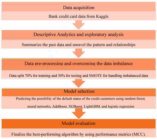
Figure 1.
Methodology framework.
3.2. Exploratory Data Analysis (EDA)
Raw data, also known as unprocessed data, are only helpful if there is something to be gained from investigating it. EDA involves analyzing and visually representing the data to gain insights, as well as summarizing significant data properties to gain a better understanding of the dataset.
According to IBM (Education 2020) and (Aswini et al. 2020), EDA gives users a more profound knowledge of the variables in the data collection and their relationships. It is generally used to explore what data might reveal beyond the formal modeling or hypothesis testing assignment. EDA can also aid in determining if the statistical approaches being considered for the research methodology are appropriate.
Some models have a significant number of features, which can cause the arrangement and training processes to take more time and consume a significant amount of system memory. It requires considerable time and effort for each feature to scan through the various data instances and estimate every potential split point, which is the primary factor contributing to this behavior. It is evident that when there are extra features in the data, the efficiency and scalability of the model are far from optimal. It is recommended to have fewer characteristics to save time during the computing process and boost the model’s performance.
The work of (Al-qerem et al. 2019) mentioned that data preparation is a crucial step when developing a classification model, as it significantly affects model accuracy. Applying feature selection techniques to a vast dataset is also of great importance; it improves accuracy and performance.
The summary statistics provided in Figure 2 help to understand the variable distribution more effectively.
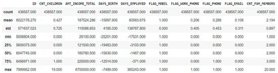
Figure 2.
Summary statistics.
Based on the observations from the above table, firstly, the variables were further analyzed, and “Flag mobile” was decided to be removed from the model prediction since the minimum and maximum value are both “1”. Secondly, outliers need to be checked for a few variables since there is a considerable difference between the maximum value and the 75th percentile value. Thirdly, the variables with the value “0” for a min, 25th, 50th, and 75th percentiles were further investigated.
Unstructured data are transformed through data visualization into groupings and metrics that may be quickly used as smart business information for quick and effective decision-making. The application submitted date and the status value for each month following the open month for the credit card help to analyze the credit behavior. The credit card customers’ past credit history can be compared during the various application months.
Additionally, it identifies relationships and patterns, as well as areas that work well or can be improved. The distribution of the variables and the data balance are examined using a variety of data visualization approaches such as bar charts, pie charts, and histograms to enhance the comprehension of the information and its aspects.
Unique values of each column were checked to identify the redundant columns. When the attribute has numerous unique values, it takes longer to conclude the data analysis, which should focus on the crucial part of our research questions. The detailed data analysis followed the steps below.
3.2.1. Performance Window and Target Variable Creation
Following the issuance of the customer’s credit card, the details of the customer will be retained in the system, and each transaction will be monitored for various reasons. One of the most critical functions of monitoring the account’s credit status is to track how much money is being spent and how much is being paid back. To maintain a credit scorecard for each month, the status must be categorized as either good or bad for each customer.
According to the algorithm, the bank or financial institution can distinguish between good and bad customers using the available features from the application filled out by the customer. In the context of this study, “bad” accounts are those whose overdue balances have a status of 2, 3, 4, or 5, while “good” accounts are all other types of accounts. The dataset needs to include information regarding the opening date of the credit card. When analyzing the data, the month with the earliest “MONTHS_BALANCE” is deemed to be the account’s opening month. Then, we reorganize the data such that month 0 represents the beginning month, and one month after the beginning month is indicated by month 1, see Figure 3.
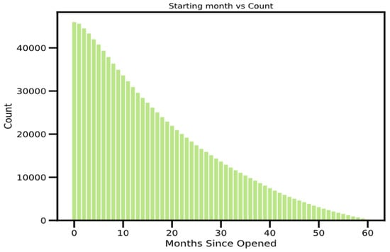
Figure 3.
Performance over the period.
Figure 4 below depicts the monthly distribution of accounts by status. It shows each account-opening month, beginning with month 1 and continuing through month 60, and helps to review the performance of the portfolio. From the time window, it is necessary to identify their status and accounts according to the month they were created.

Figure 4.
Bad rate of the portfolio.
Over the course of all account-opening months, the bad rate ratio needs to be computed for the entire portfolio to locate the stable period of the bad rate. In the beginning, there was only a modest increase in the number of credit cards; however, this may have been insignificant for the models. Figure 4 shows that accounts that have been open for more than 50 months demonstrate a dramatic increase in the percentage of bad loans.
As previously indicated, the status column contained various values that had been converted to binary numbers. The status values 2, 3, 4, and 5 are changed to 1, while the others are set to 0. A “bad customer” is one whose past-due balance exceeds 59 days, while a “good customer” is one whose past-due amount is less than 60 days. According to the binary value, 1 represents a bad customer, whereas 0 represents a good one.
As per the time series graph shown in Figure 5, the bad rate has nearly stabilized after one year (12 months). Based on this, the first 12 months can be considered as a performance window or the time frame for the analysis. Any customers that go delinquent within the first year will be labeled as “bad,” while the remainder will be considered “good”. Customers are categorized as bad or good based on their status throughout the initial 12 months, as shown in Figure 5.
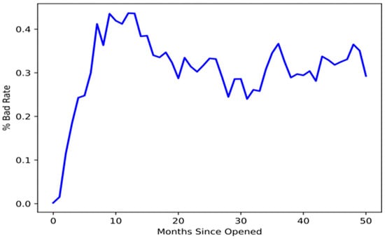
Figure 5.
Bad rate of the portfolio after one year.
3.2.2. Target Distribution
According to Figure 6 below, the data are exceptionally imbalanced, with a rate of 1.3% for bad customers.
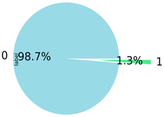
Figure 6.
Target distribution.
3.2.3. Handling Outliers
Outliers can affect the quality of the research since all statistical data are susceptible to their effects, including means, standard deviations, and all other statistical inferences based on them. Handling outliers is one of the essential steps in data pre-processing. According to Figure 7 below, there are outliers that need to be removed from the data regarding days employed, total income, count of children, and count of family members.
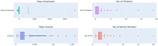
Figure 7.
Box plots of features.
Outliers for the columns’ days employed, the number of children, total income, and number of family members are detected using box plots, as shown above, and handled using the IQR method. The IQR method is used to detect the outliers by setting up a bar outside Q1 and Q3. Weights that fall beyond the fence range are concluded as outliers. To construct the fence results, we multiplied the IQR by 1.5, subtracted this amount from Q1, and added it to Q3. Outliers are any observations that exceed 1.5 IQR below Q1 or more than 1.5 IQR above Q3. Then, outliers were removed to ensure they did not impact the model’s outcomes, as shown in Figure 8.
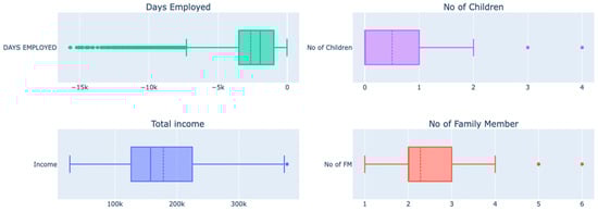
Figure 8.
Box plots of features after removing outliers.
The missing values were analyzed, and 32% of the values were missing in the variable “OCCUPATION_TYPE”. With the account-opening month and date of birth, the age and months of experience as of the application date are calculated backward from the application date to the date of birth and from the application date to the months of experience, respectively.
3.2.4. Data Visualization
The boxen plot and box plot, as displayed in Figure 9, are used to compare and understand the distribution of essential variables and the status of the customer.
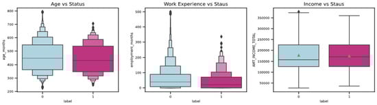
Figure 9.
Distribution of important variables.
The observations from the graphs above are as follows:
According to the first graph, the younger population, in general, poses a greater risk than the older population. It is evident that banks and other financial institutions should consider a person’s age when deciding whether to issue them a credit card.
- The second graph shows that people with less experience typically pose a greater risk than those with more experience. When issuing a card, banks and other financial organizations should consider experience as one of the factors.
- As per the third graph, the red square refers to the average income, showing that the average income of the bad customers is below the average income of the good customers.
- It is evident from the pie charts shown in Figure 10 below that good customers have a higher proportion of property ownership compared to bad customers.
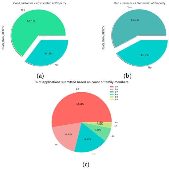 Figure 10. Pie charts of features. (a) Good customer vs. ownership of property; (b) bad customer vs. ownership of property; (c) applications vs. family members.
The histograms in Figure 11 show the distribution of the numeric variables for the most important variables:
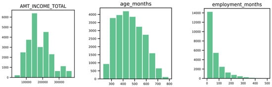
Figure 11.
Histograms of features.
- The income total shows the highest distribution between 50,000 and 275,000.
- Age shows the highest distribution between 300 months and 600 months, which is 25 to 50 years.
- Employment months have the highest distribution between 0 and 50 months, less than 1 year to 4 years.
The correlation matrix, illustrated in Figure 12 below, is a chart that displays the correlation coefficients established between different sets of variables. The table shows the correlation between each variable and each value. This makes it possible to identify the pairs with the highest correlation. In the study, a correlation matrix is initially generated to determine how each pair of variables relates to one another. It should be considered to remove variables if there is a significant relationship between them; hence, a set of highly correlated characteristics will not contribute any new information or very little. Moreover, they will complicate the algorithm and increase the possibility of errors. It is beneficial to remove the variables that are significantly correlated with one another in order to reduce memory and speed issues. According to the confusion matrix presented below in Figure 12, the number of children and family members is highly correlated with a correlation of 85%. Initially, it was decided to remove one of the strongly correlated variables; however, both variables are kept for analysis because the correlation is less than 90%. Also, even after keeping both variables in the research, there is no adverse impact on the performance metrics results.
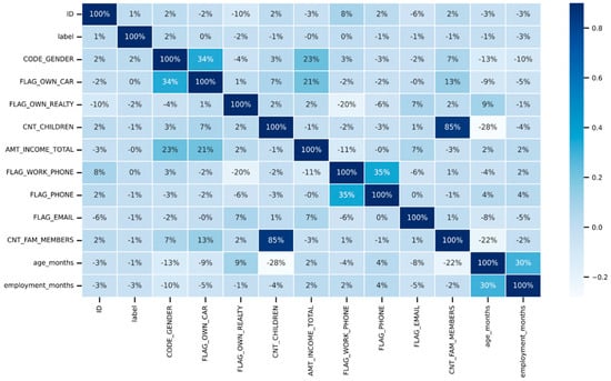
Figure 12.
Correlation matrix.
3.3. Data Pre-Processing
One of the early pre-processing procedures that must be carried out in machine learning is splitting the modeling dataset into training and testing samples. Testing the model on the test set after training it on the training set will assist in determining how effectively the model generalizes to brand-new, untainted data. The training and testing sections of the dataset used in this study were split in a proportion of 70% training and 30% testing (70:30). Thirty percent of the data were utilized to assess the learning effectiveness of the testing data, while seventy percent of the datasets were utilized as a training set, ensuring that the training model was not exposed to the test sets.
When working with the classification model, the most significant problem is the unequal distribution of the values across the dataset. This is the fundamental issue. The same pattern is shown in the research data, where the distribution of good customers is 98.7% and bad customers are 1.3% (Figure 6). Most traditional machine-learning techniques assume that the distributions of the target classes are uniform. This impacts the models’ performance because unbalanced datasets will cause these models to underperform. As a result, a higher accuracy for large categories (as in our case, good customers) and a lower accuracy for smaller classes (bad customers) may result from the direct input of unbalanced data. Even though the performance metrics show a good accuracy in this circumstance, other performance metrics will not show high enough ratings in other evaluation criteria. Two methods can resolve this issue. The first one is undersampling, which deletes the dominant values, and the second is oversampling, which adds rare values to the dataset. Undersampling strategies such as IB3, DROP3, and GA and oversampling strategies such as SMOTE, CTGAN, and TAN can be used to handle unbalanced data.
SMOTE is an oversampling method, one of the better ways of handling imbalanced data by producing fictitious samples for the minority class. This strategy assists in overcoming the issue of overfitting caused by random upsampling. It focuses on the feature space to generate new instances using interpolation between positive occurrences that are close together. The issue is handled and sorted by using the mentioned upsampling method, SMOTE. It involves adding artificially generated data records corresponding to the minority class into the dataset. After the upsampling procedure, the counts for the two labels are almost identical and can be used for predictive modeling.
According to our data, SMOTE can tackle the imbalanced target variance issue, and the testing data show that the distribution is likewise balanced, with 7355 “good customers” and 7473 “bad customers”.
4. Machine-Learning Algorithms
The models presented below serve as illustrations of supervised machine-learning techniques utilized in the analysis. They are used to select the most appropriate classification model to classify good customers from bad customers, contributing to the credit card industry.
4.1. Random Forest
Prior to discussing the details of the random forest model, it is vital to define decision trees, ensemble models, and bootstrapping, all of which are fundamental to an understanding of the random forest model (Beheshti 2022). The decision tree is an application of supervised machine learning. It provides a flow chart type/tree-like structure, making it simple to visualize and extract information from the background process (Sharma 2023).
According to (Meltzer 2023), multiple decision trees are grown using random forests and combined to produce a more precise prediction, see Figure 13. The random forest algorithm develops trees while simultaneously introducing more randomness to the system. This method finds the best variable from a random collection of features when partitioning a node instead of selecting the element that is regarded as the most essential. This ends up providing vast diversity, which, in many circumstances, leads to a better model. As a result, in a random forest, the method used to divide a node will only consider a random subset of all the characteristics (Donges 2021).
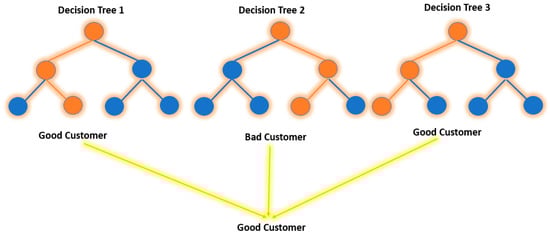
Figure 13.
Decision tree.
The pseudo-code for the random forest model is shown in Algorithm 1 to elucidate the mechanism by which random forests operate. The algorithm describes a structured approach to random forests, which use bootstrap sampling to generate individual trees, which are then combined to form the overall forest.
| Algorithm 1. Random Forest Algorithm |
| Precondition: A training set , features , and number of trees in forest .
|
One of the hyperparameter tuning parameters is referred to as the “Criterion”. The Gini index is set as the default parameter for the random forest. The Gini index is used to determine the node distribution on a decision tree branch.
where
- = the probability of picking the data point with the class i;
- c = number of classes.
4.2. Logistic Regression
Logistic regression is one of the supervised machine-learning algorithms classified as a subset of linear regression. However, it is solely employed for categorization. Logistic regression completes binary classification tasks by estimating the likelihood of a given outcome, event, or observation. In our work, the model produces a binary outcome with only two options: good customer or bad customer, based on the status.
The pseudo-code for the logistic regression algorithm is shown in Algorithm 2. It splits data into different individual groups and examines the association between one or many independent features. It is frequently applied in the field of predictive modeling, in which the model determines the mathematical likelihood of whether or not a particular occurrence belongs to one specific category. As per our case, 0 is denoted as “good customer” and 1 is denoted as “bad customer”. The sigmoid function is an activation function of logistic regression, and logistic regression employs the sigmoid function to establish a link between predictions and probabilities.
| Algorithm 2. Logistic Regression |
Logistic Regression
|
As shown in Algorithm 3, any real number can be transformed into a range of 0 and 1 using a function called the sigmoid, represented by an S-shaped curve. The sigmoid function’s output is regarded as 1 if it is greater than 0.5. On the other side, the output is categorized as 0 if it is less than 0.5. The formula of the sigmoid function is as follows:
where e = base of the natural logarithms.
| Algorithm 3. Sigmoid Function |
| Sigmoid Function Require: Training data , number of epochs , learning rate η, standard deviation σ Ensure: Weights
|
Logistic regression is demonstrated by the following equation:
where
- x = input value;
- y = predicted output;
- = bias or intercept term;
- = coefficient for input (x).
Parallel to linear regression, the above equation predicts the output value (0 or 1) by linearly integrating the input values using weights or coefficient values.
4.3. Neural Network
The model for predicting credit risk is developed using an artificial neural network, which has a structure with three layers called input nodes, hidden layers, and output layers, as illustrated in Figure 14. According to the dataset, customer details are the input nodes, and customer classifications such as “good customer” or “bad customer” are the output nodes.
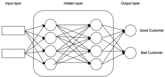
Figure 14.
Neural network.
Training data are received by the input layer and passed to the hidden layers to convert the raw data into characteristics with a high dimension that are nonlinear, and then the output layer classifies the data. Firstly, the algorithm will be used to train the ANN-based classifier based on historical information. Later, the algorithm will be used to determine the customer’s credit risk.
Generally, a neural network begins with a random set of weights. Each time the network finds an input–output pair, it modifies its weights based on it. Each pair passes through two processing phases: a forward pass and a backward pass. The forward pass involves delivering a representative input to the network and allowing activations to flow until they reach the output layer. The standard backpropagation is a gradient descent algorithm that repeats steps in the reverse direction to adjust the model’s parameters based on weights and biases.
The algorithm’s first iteration step can be expressed as follows:
where
- W(t) = vector of the weights at iteration step t;
- ∇E(t) = current gradient of the error function;
- E = sum of the squared errors;
- μ = learning rate.
The learning model updates the gradient descent weights with more momentum (β) in order to shorten the training time.
where
- ΔW(t) = current adjustment of the weights;
- ΔW(t − 1) = previous change to the weights;
- β = momentum.
Momentum enables a network to deploy to recent trends in the error surface and local gradient. It permits the network to dismiss small elements in error; it functions like a low-pass filter. Through the use of the first-order and also second-order derivatives of μ and β, the learning rates and momentum are updated with optimum rates during the training process. Each iteration of the backpropagation algorithm allows for the quick and easy computation of these derivatives. After the training, the model can be used to distinguish the riskiest customers by analyzing customer data.
To comprehend the intricate patterns that lie beneath the surface, deep-learning algorithms require an adequate quantity of data. When more data are used, the performance of deep-learning models will significantly improve.
4.4. XGBoost Algorithm
XGBoost (see Figure 15) is a widely used implementation of the gradient-boosted tree technique that is both efficient and open-source. Gradient boosting is a method of supervised learning that accurately predicts a target variable by combining the predictions of a series of weaker, simpler models.

Figure 15.
XGBoost.
According to (Kharwal 2020), gradient boosting works well by minimizing loss when adding new models. Regression trees serve as the weak learners in gradient boosting for regression to translate each input parameter to a leaf that has a continuous value. XGBoost minimizes a systemized objective function by integrating the convex algorithm based on the variance between the anticipated and target outcomes and a penalty element for model complexity. The training procedure is carried out repeatedly by adding additional trees that reveal the residuals or mistakes of older trees, which are then incorporated with earlier trees to produce the final forecast.
where
- αi—regularization parameters;
- r—residuals computed with the ith tree;
- hi—function trained to predict residuals;
- ri—using X for the ith tree.
- Residuals and Arg(minα) have to be computed in order to compute the α.
where
where
- L(Y, F(X)) is the differentiable loss function.
4.5. LightGBM Algorithm
LightGBM represents a gradient-boosting framework created on decision trees (a tree-based algorithm that grows leaf-wise, as shown in Figure 16, rather than level-wise) for the light gradient to reduce memory usage, enhance memory utilization, and increase the model’s efficiency.
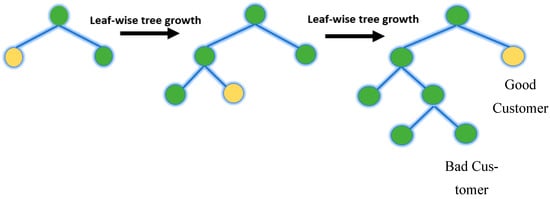
Figure 16.
LightGBM.
As per (GeeksforGeeks n.d.), LightGBM employs two methods: EFB (Exclusive Feature Bundling) and GOSS (Gradient-based One-Side Sampling), which collectively enable the model to function effectively. GOSS will merely use the remaining data to evaluate the overall information gain, excluding the extensive number of data sections that have insignificant gradients. The calculation of statistics expansion gives more weight to the data instances with significant gradients. Despite utilizing a smaller dataset, GOSS can produce trustworthy findings with substantial information gain compared to other models. It has gained popularity due to its high speed and ability to handle large amounts of data with low space complexity. Although EFB rarely receives any non-zero values parallel to shrinking the number of characters, it does put the mutually exclusive features along with frivolity. This affects the total outcome for efficient feature elimination without compromising the split point’s accuracy. Any algorithm’s training time will be shortened by 20 times by combining the two improvements. With EFB and GOSS together, LGBM can be considered gradient-enhancing trees. It performs best with massive data.
LightGBM and XGBoost vary primarily in that whereas XGBoost employs a histogram-based method and a pre-sorted algorithm for the most effective division calculation, LightGBM selects data instances to calculate a split value using the GOSS technique. LightGBM employs a highly optimized decision-making algorithm that is based on histograms and offers significant advantages while also being efficient and memory-efficient.
The critical characteristics of LGBM include higher accuracy and faster training speeds, low memory usage, superior comparative accuracy to other boosting algorithms, better handling of overfitting when working with smaller datasets, support for parallel learning, and compatibility with small and large datasets.
Decision tree-based machine-learning algorithms were formerly the industry standard. The best solutions for the majority of problems used XGBoost. Microsoft unveiled its gradient-boosting technology, LightGBM, a few years ago. Currently, it takes center stage in gradient-boosting devices. XGBoost has been replaced by LightGBM.
4.6. AdaBoost Algorithm
A common boosting approach called AdaBoost aids in combining several “weak classifiers” into one “strong classifier”. In other words, to improve weak classifiers and make them stronger, AdaBoost employs an iterative process. AdaBoost is a form of ensemble learning approach. Based on the output of the previous classifier, it aids in selecting the training set for each new classifier. It establishes how much weight must be assigned to each classifier’s suggested response when the results are combined.
Algorithm 4 clarifies the AdaBoost methodology. Initially, all data points are equally weighted. However, as the algorithm progresses through each iteration, it meticulously recalibrates the weights of incorrectly classified data points. This weight adjustment ensures that subsequent classifiers prioritize those specific misclassified instances, thereby improving the cumulative prediction accuracy. At the end of the iterative process, AdaBoost merges the outcomes of all weak classifiers and weights them according to their respective accuracies to produce a robust final classifier.
| Algorithm 4. AdaBoost |
| AdaBoost Algorithm Given: . Initialize: For :
|
The research by (Nazarenko et al. 2019) highlighted the benefits of AdaBoost:
- Good generalization skills: Creating compositions for real-world issues of a higher caliber is more feasible than using the fundamental algorithms. As the number of fundamental algorithms rises, the generalization ability may become more effective (in some missions).
- Own boosting expenses are minimal: The training time of the fundamental algorithms nearly entirely determines the amount of time needed to construct the final image.
- Several drawbacks of AdaBoost can be discussed as follows:
- Boosting technology develops gradually: It is crucial to guarantee high-quality data.
- Tactful to unorganized data and outliers: Hence, it is intensely advised to avoid these before using AdaBoost.
- Slower than XGBoost: It has also been indicated that AdaBoost is slower than XGBoost.
Hyperparameter tuning aims to train each model and finalize the best-predicting model. In the modeling process, one critical aspect that needs to be considered is whether there is still potential for improvement before completing the best-performing model. As a result, the model needs to be improved in whatever manner possible. Hyperparameters are one of the key elements in performance improvement. The performance of these models can be considerably improved by selecting the appropriate values for their hyperparameters, which are critical to how effectively they function. Table 2 represents the hyperparameters set for each model for the predictions.
Table 2.
Hyperparameter for each methodology.
5. Implementation and Results
In this section, we first introduce confusion matrix, which is the framework that we adopted; and then we will discuss the results from implementing our chosen machine-learning algorithms. Further analysis will also be investigated from the best-performing model.
5.1. Confusion Matrix
The confusion matrix, shown in Figure 17, is a technique for determining the effectiveness of a classification algorithm. Classification accuracy is defined as the proportion of accurate predictions compared to all other predictions. A better understanding can be obtained of what the classification model is doing correctly and the mistakes it makes by calculating a confusion matrix. The total number of precise predictions for a class is recorded in both the predicted column and true label row for that class value. Likewise, the total amount of imprecise predictions for a class is recorded in both the predicted column and the actual label row for that class value. Confusion matrices attempt to differentiate the occurrences with a specific outcome.
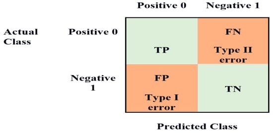
Figure 17.
Confusion matrix.
The binary classification problem distinguishes between observations with a particular outcome and regular observations. Based on our model predictions, the customers will become default or not in the loan defaulting prediction. The good customer is labeled as “0” and the bad customer as “1” in this matrix.
This results in the following:
- True positive—When good customers are accurately predicted as good customers.
- False positive—When bad customers are improperly predicted as good customers.
- True negative—When bad customers are accurately predicted are bad customers.
- False negative—When good customers are improperly predicted as bad customers.
The equations to compute the respective rates are as follows:
- True positive = Number of customers accurately predicted as good/Actual number of good customers
- False positive = Number of customers improperly predicted as good/Actual number of bad customers
- True negative = Number of customers accurately predicted as bad/Actual number of bad customers
- False negative = Number of customers improperly predicted as bad/Actual number of good customers
According to the test samples, 7422 are good customers, whereas 7406 are bad customers. Based on the number of actual good and bad customers for the prediction algorithm, we will analyze the false positive rate, true positive rate, false negative rate, and true negative rate for the best-performing and worst-performing algorithms.
5.2. Implementation and Comparison of Machine-Learning Algorithms
The neural network model forecasted all customers as good, as shown in Figure 18. As a result, a total of 5918 bad customers were inaccurately predicted as good customers. In addition, none of the bad customers were correctly predicted as bad customers by the neural network. Consequently, the false positive rate ended up being 80%, whereas the true negative rate was 20%.
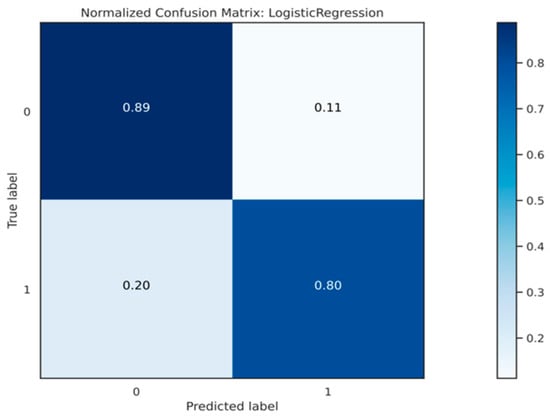
Figure 18.
Confusion matrix—Logistic regression.
Since the model projected that nearly all consumers would be good, the true positive rate is calculated as 89%. Moreover, the model incorrectly projected 0 customers as bad customers when they were actually bad customers, resulting in a false negative rate of 20%.
The XGB model correctly predicted both 7406 good customers and 7320 bad customers, as shown in Figure 19. Consequently, the true positive rate ended at 99.50%, whereas the true negative rate ended at 96.27%. In addition, the model incorrectly projected 278 customers as good customers when they were bad customers. Additionally, the model incorrectly predicted that 37 customers were bad when they were good customers.
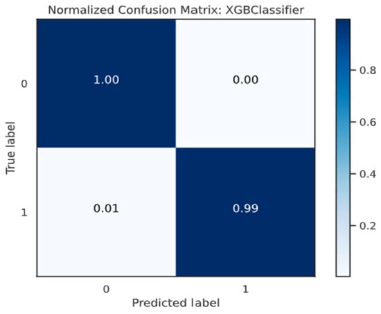
Figure 19.
Confusion matrix—XGBoost.
As per the confusion matrix, XGBoost displays a superior performance, while the neural network does not perform well for this purpose. Other performance metrics are also vital to know how the model performs in the prediction scenario. This examination focuses on classifier evaluation metrics, including AUC, accuracy, recall, and precision.
5.2.1. Accuracy
Accuracy is the easiest and most well-known measure for classification problems. It is calculated by dividing the number of accurate predictions by the overall number of forecasts. Further, while discussing accuracy, true negative rate (TNR), true positive rate (TPR), false negative rate (FNR), and false positive rate (FPR) also need to be considered. Accuracy can be computed as follows:
As shown in Figure 20, the bar chart of accuracy comparison reveals that XGB has the highest accuracy, coming in at 99.4%, followed by LGBM, which has a good accuracy of 99.3%, and finally, logistic regression, which has the lowest accuracy, coming in at 84.3%.
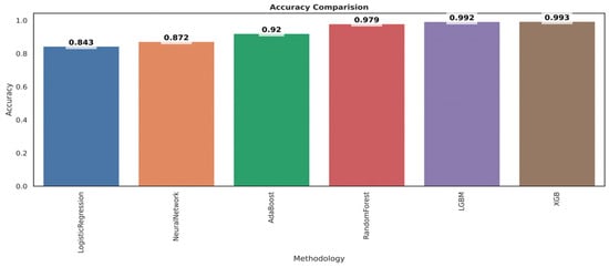
Figure 20.
Performance evaluation.
However, accuracy alone does not tell the entire story when dealing with a class-unbalanced dataset, where there is a considerable variance between the total number of positive and negative labels. Therefore, other performance metrics are also further analyzed.
5.2.2. Recall and Precision
Precision and recall apply to individual classes only; for instance, recall for good customers or precision for bad customers.
Precision attempts to answer the question, “What percentage of positive identifications were actually accurate?” The basis for precision is prediction. To explain, how many were correctly predicted as bad customers out of all the bad customer predictions? Or how many were correctly predicted as good customers out of all the good customers’ predictions?
The mathematical equation for precision is as follows:
Recall attempts to answer the question, “What percentage of true positives were correctly detected?” The basis of the recall is the truth. That is, out of all the bad customers, how many were predicted as actually bad customers? Or, out of all the good customers, how many were predicted as actually good customers?
The mathematical equation for the recall is as follows:
Precision or recall should be chosen depending on the problem that needs to be solved. Use precision if the issue is sensitive to classifying a sample as positive in general, including negative samples that were mistakenly categorized as positive. Use recall if the objective is to find every positive sample without minding whether some negative samples could be mistakenly categorized as positive. In our situation, identifying bad customers is very similar to identifying good customers. According to this, precision is critical in our scenario.
The precision and recall comparison bar charts in Figure 21 and Figure 22, respectively, make it evident that the model XGB has the highest possible precision as per Figure 21 and recall as per Figure 22 (both are 0.994), followed by the model LGBM (both are 0.992 and 0.993). In addition, the logistic regression has the lowest score for both precision (0.846) and recall (0.843).
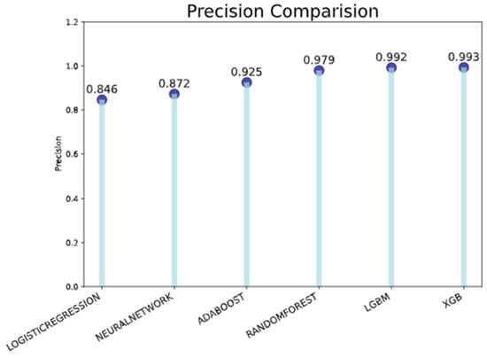
Figure 21.
Precision comparison.
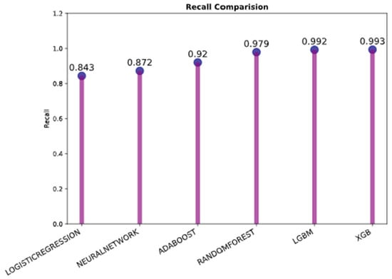
Figure 22.
Recall comparison.
5.2.3. F1 Score
Another performance metric is the F1 score, which ranges from 0 to 1 and is a harmonic average of recall and precision. The most recommended quality metric for a binary classification task is to optimize for its F1 score. The higher the F1 score, with 0 being the worst and 1 being the highest, the better the overall performance of the model. Only when precision and recall are both 100% does it attain its ideal level of 1. The F1 score has its worst value of 0 if one of them is equal to 0.
F1 = 2 × ((Precision × Recall)/(Precision + Recall))
The scenario is reflected in Figure 23 in the same way as recall and precision discussed earlier. It is clear from this that the model XGB achieves the highest possible F1 score due to the fact that the XGB achieves the highest possible recall and precision.
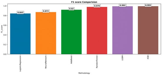
Figure 23.
F1 score.
5.2.4. ROC Curve and AUC Score
The ROC curve and AUC score are among the most crucial evaluation systems for measuring the performance of classification models. The ROC curve is a probability curve, and the AUC defines the degree or measure of separability. It describes how well the model differentiates between classes. The greater the AUC, the better the model predicts bad credit card customers as bad and good credit card customers as good. In summary, the greater the AUC, the better the model differentiates between good and bad credit card customers. The following two factors make AUC desirable:
- Scale is unimportant to AUC: It evaluates how well predictions are ranked rather than the absolute values of the predictions.
- AUC is independent of the classification threshold: It evaluates how well the model predicts regardless of the classification threshold.
The baseline of the ROC curve can be explained at the diagonal points by default (FPR is equal to TPR). TPR is mapped against FPR on the ROC graph, with FPR on the x-axis and TPR on the y-axis. Algorithms closer to the top left corner corresponding to the coordinate (0, 1) in the Cartesian plane demonstrate a better performance than those below.
The test will be less precise the closer the graph gets to the ROC plot’s 45-degree diagonal. The fact that the ROC curve does not depend on the class distribution is one of the many reasons it is so valuable. It enables and facilitates situations in which the classifiers predict unusual events, which is the same as our concern regarding the detection of bad customers.
The value of AUC ranges from 0 to 1. An AUC of 0 specifies a model with 100% incorrect predictions, while an AUC of 1 indicates a model with 100% correct predictions. If the area under the curve AUC is equivalent to 0.5, then we can conclude that the algorithm is incapable of differentiating between good customers and bad customers accordingly.
On an ROC curve, a greater value on the x-axis specifies a more significant number of false positives than true negatives. At the same time, a higher value on the y-axis also represents a more significant proportion of true positives than false negatives. Accordingly, threshold selection depends on the capacity to create an equilibrium between false positives and negatives. Model comparison of random forest, neural networks, XGB, LGBM, AdaBoost, and logistic regression is as follows.
As per Figure 24, LGBM and XGB show a better performance. The best models for correctly classifying observations are LGBM and XGB, which have the most significant AUC and the highest space below the curve. The green line indicates the model LGBM and is embedded behind the red line model XGB; after XGB and LGBM, random forest and AdaBoost perform best—in that order. Logistic regression is near the points lying around the diagonal, and the neural network is on the diagonal line, which indicates a poor performance.
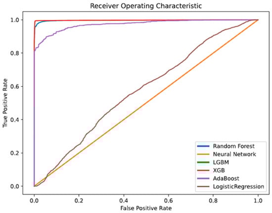
Figure 24.
ROC–AUC curve.
As per Figure 25 below, the red line of XGBoost at the (0, 1) position in the upper left corner of the Cartesian plane exhibits a superior performance.
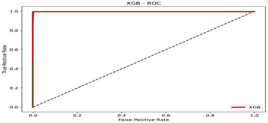
Figure 25.
ROC—XGB.
As a result of our analysis of ROC–AUC, we are able to draw the conclusion that LGBM and XGB outperform the other algorithms in terms of their ability to identify good customers as good and bad customers as bad.
5.2.5. MCC
A class imbalance can affect accuracy, recall, precision, and F1 score, making them all uneven. An alternative approach to binary classification is to treat the true class and the predicted class as two different variables and calculate their correlation coefficient similarly to compute the correlation coefficient between any two variables. MCC aids in identifying the classifier’s shortcomings, particularly with regard to the negative class samples. MCC is a single-value statistic that distills the confusion matrix, much like the F1 score. No class is more significant than any other since MCC is also totally symmetric; even when the positive and negative values are switched, the result remains the same. A high number, near 1, indicates that MCC correctly predicts both classes. In other words, a score of 1 represents complete agreement. Even if one class is unreasonably under-represented or over-represented, MCC considers all four values in the confusion matrix. Following this, there are calculations for MCC:
By looking at their equations, one can quickly determine the main advantage of employing MCC instead of the F1 score. The number of true negatives is ignored by the F1 score. Conversely, MCC is gracious enough to take care of all four entries in the confusion matrix. MCC is favored over the F1 score only if the cost of low precision and low recall is truly unknown or unquantifiable because it is a “fairer” evaluation of classifiers, regardless of which class is positive.
MCC is the best single-value classification metric, which serves to summarize the confusion matrix or an error matrix. As per Figure 26, the model XGB outperforms the other algorithms with a score of 0.9879, followed by LGBM (0.986).
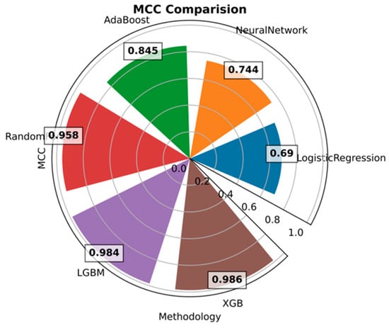
Figure 26.
MCC evaluation.
5.3. Comparison of the Best- and Worst-Performing Models
According to Figure 27, random forest is superior in its ability to differentiate between good and bad customers. The best scores assure the breakdown results for both good customers (0) and bad customers (1) with the other performance metrics, such as precision (0–0.965 and 1–0.995), recall (0–0.995 and 1–0.964), and f1 score (0–0.980 and 1–0.979).
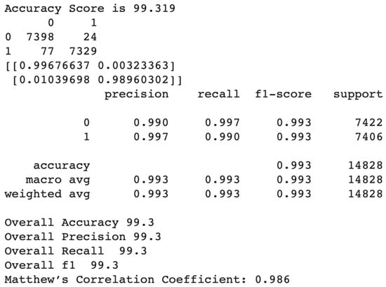
Figure 27.
Summary of the best-performing model.
The following Table 3 represents the summary of all performance metrics for each algorithm.
Table 3.
Summary of performance metrics.
Finally, we look at the feature importance from the best-performing model XGBoost, and the results are shown in Figure 28 below, which indicates how each feature contributes to the classification prediction model of XGBoost.
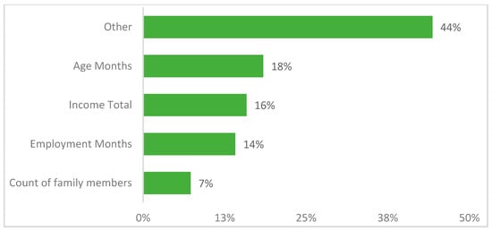
Figure 28.
Feature importance of XGBoost.
A feature with a higher value indicates that it is more crucial than a feature with a lower value in predicting the customer type. In addition, the inclusion/exclusion of this feature from the training set significantly impacts the final results. As per the figure above, the customer’s age, income total, employment months (experience), and count of family members are the crucial features of the XGBoost model formation. Also, other features only contribute around 13% to the model.
6. Further Discussion
From the experimental results in this section, the XGBoost model demonstrated high accuracy on the selected dataset; this is in line with the recent literature on credit risk modeling, which emphasizes the importance of dynamically robust machine-learning models that maintain performance over time. The work of (Shi et al. 2022) discusses various computing techniques, including traditional statistical learning, machine learning, and deep learning, highlighting how these models have evolved to meet the demands of credit risk prediction. The authors underscore the necessity for the continuous adaptation of these models to new data and market changes, reinforcing the idea that model robustness is critical for real-world financial applications. Similarly, research by (Alonso Robisco and Carbó Martínez 2022) focuses on the model risk-adjusted performance of machine-learning algorithms in credit default prediction, identifying the potential risks when models overly depend on specific datasets. The study explores the application of interpretability techniques, such as SHAP and LIME, to ensure that models can be regularly evaluated and validated against changing market conditions. It also proposes methodologies to quantify model risk, underscoring the need for dynamic evaluation processes to ensure models remain effective and compliant with regulatory standards.
It is crucial to recognize that credit risk profiles evolve over time due to various factors, including economic fluctuations and changing consumer behaviors. To maintain accuracy and robustness, models should be periodically retrained with new data to adapt to these changes.
7. Conclusions
7.1. Summary
Collecting payments from bad customers is a significant challenge for banks and financial institutions, leading to prolonged collection processes and high expenses. One of the most crucial decisions for these organizations is accurately identifying customers who are both willing and capable of repaying their debts. This research contributes to this decision-making process by developing a model to predict the credit risk of credit card customers.
By addressing outliers and selecting essential features, various machine-learning models were applied to a credit dataset. Among the models examined, XGBoost outperformed others in terms of all performance metrics, including accuracy, precision, recall, ROC–AUC, F1 score, and MCC.
The proposed XGBoost model can effectively predict the default status of credit card applicants, aiding banks and financial institutions in making more informed decisions. By implementing this model, banks can enhance the accuracy of their credit risk assessments, resulting in higher acceptance rates, increased revenue, and reduced capital loss. This approach allows financial institutions to operate efficiently, maximizing profits while minimizing costs.
For banks and financial regulators, this research has real advantages. Lenders can improve their credit approval procedures and possibly lower default rates and related losses by putting the XGBoost model into practice. For example, over a twelve-month period, a large bank that tested a comparable methodology experienced a 15% drop in defaults. These insights could be used by regulators to revise credit risk assessment rules, guaranteeing that banks continue to employ sound evaluation techniques. Machine-learning models are already being considered by one regulatory authority as a requirement for standard credit checks. Additionally, the model’s capacity to pinpoint important risk indicators may aid in the development of more focused financial education initiatives that target particular default risk-causing behaviors.
7.2. Recommendations
In light of the insights obtained from this study, it is recommended that credit card issuers or banks incorporate this predictive credit risk analytics into their operations for strategic business and marketing decisions. Firstly, this method segments cardholders based on credit risk, allowing credit card issuers or banks to enhance their credit risk management by avoiding or decreasing the number of non-payers. Secondly, with a clear understanding of all the customers’ creditworthiness, credit card issuers or banks can identify those most likely to responsibly address increased credit lines or additional financial products. This can lead to effective upselling and cross-selling strategies, thus increasing the customer lifetime value and overall revenue growth. Thirdly, credit card issuers or banks can implement a risk-based pricing strategy by accurately classifying card holders according to their credit risk. This may involve offering better terms to low-risk customers, enhancing customer retention, and attracting other creditworthy customers. Fourthly, economic fluctuations can affect the financial stability of cardholders and, therefore, their credit risk. The predictive credit risk analytics can quickly incorporate these changes by monitoring a customer’s financial situation over a period of six months or even longer. This enables card issuers or banks to adjust their strategies accordingly, demonstrating resilience and flexibility in volatile market conditions.
Our research findings have pragmatic and practical implications for credit card companies, banks, and financial institutions, significantly improving lending decisions by leveraging the ML models, such as LGBM and XGBoost, to predict credit risk. Financial institutions can identify high-risk applicants to minimize bad debt and write-offs. Similarly, they can approve creditworthy customers to expand the market share. Increased predictive power also enables personalized loan terms based on an applicant’s true default risk.
7.3. Limitations of the Study and Future Work
This research could be enhanced by incorporating more recent and diverse credit card data, which should include a wider range of features. Additionally, considering the acquisition of a dataset with a larger number of records would improve the robustness of the model.
The SVM algorithm was also attempted for prediction. However, it was excluded from this study because it required a significant amount of time (more than 2 h) to run, making it an expensive model in terms of computational resources.
The default credit status is influenced by macroeconomic factors such as the inflation rate, interest rate, GDP (gross domestic product), and unemployment rate. Future data collection efforts should incorporate these macroeconomic factors to enhance the prediction of credit card default status.
In subsequent work, the K-fold validation methodology should be incorporated, in addition to the machine-learning classifiers used in this study. This would add a new dimension to the prediction method, employing the latest techniques and expandable AI to better identify customers with good credit records.
Future work should also explore adaptive learning methods, such as online learning, that can dynamically adjust model parameters in response to new data patterns. Additionally, continuous performance monitoring in real-world applications is recommended to promptly identify and address any declines in model accuracy.
Author Contributions
Conceptualization, V.C. and S.S.; methodology, V.C.; software, S.S.; validation, V.C., H.W., and S.T.W.; formal analysis, V.C., S.S., and H.W.; investigation, V.C. and S.S.; resources, V.C.; data curation, S.S.; writing—original draft preparation, V.C. and S.S.; writing—review and editing, V.C., H.W., S.T.W., and J.L.; visualization, V.C., S.S., and M.A.G.; supervision, V.C. and M.A.G.; project administration, V.C.; funding acquisition, V.C. All authors have read and agreed to the published version of the manuscript.
Funding
This research is partly funded by VC Research [(VCR 0000209)] for Victor Chang.
Data Availability Statement
Data are available on https://www.kaggle.com/code/rikdifos/eda-vintage-analysis/data, accessed on 1 July 2024.
Acknowledgments
Authors are grateful to Qianwen Ariel Xu and Karl Drazar Hall, who helped to improve the quality of the paper in the early stage.
Conflicts of Interest
The authors declare no conflict of interest.
Appendix A
The explanation and remarks are obtained from https://www.kaggle.com/code/rikdifos/eda-vintage-analysis/data (accessed on 1 July 2024) for both datasets.
References
- Adha, Risfian, Siti Nurrohmah, and Sarini Abdullah. 2018. Multinomial Logistic Regression and Spline Regression for Credit Risk Modelling. Journal of Physics: Conference Series 1108: 012019. [Google Scholar] [CrossRef]
- Ali, Mohsin, Abdul Razaque, Joon Yoo, Uskenbayeva R. Kabievna, Aiman Moldagulova, Satybaldiyeva Ryskhan, Kalpeyeva Zhuldyz, and Aizhan Kassymova. 2024. Designing an Intelligent Scoring System for Crediting Manufacturers and Importers of Goods in Industry 4.0. Logistics 8: 33. [Google Scholar] [CrossRef]
- Alonso Robisco, Andrés, and José Manuel Carbó Martínez. 2022. Measuring the model risk-adjusted performance of machine learning algorithms in credit default prediction. Financial Innovation 8: 70. [Google Scholar] [CrossRef]
- Al-qerem, Ahmad, Ghazi Al-Naymat, and Mays Alhasan. 2019. Loan Default Prediction Model Improvement through Comprehensive Preprocessing and Features Selection. Paper presented at the 2019 International Arab Conference on Information Technology (ACIT), Al Ain, United Arab Emirates, December 3–5. [Google Scholar]
- Aswini, Ravichandran, Balamurugan Muruganantham, Santosh Kumar, and Arumugam Murugan. 2020. Exploratory Data Analysis for Social Big Data Using Regression and Recurrent Neural Networks. Webology 17: 922–36. [Google Scholar] [CrossRef]
- Bao, Wang, Ning Lianju, and Kong Yue. 2019. Integration of unsupervised and supervised machine learning algorithms for credit risk assessment. Expert Systems with Applications 128: 301–15. [Google Scholar] [CrossRef]
- Behera, Sudersan, Sarat Chandra Nayak, and Annadanapu Pavan Kumar. 2023. A Comprehensive Survey on Higher Order Neural Networks and Evolutionary Optimization Learning Algorithms in Financial Time Series Forecasting. Archives of Computational Methods in Engineering 30: 4401–48. [Google Scholar] [CrossRef]
- Beheshti, Nima. 2022. Random Forest Classification. Available online: https://towardsdatascience.com/random-forest-classification-678e551462f5 (accessed on 31 October 2024).
- Bindal, Anirudh, and Sandeep Chaurasia. 2018. Predictive Risk Analysis For Loan Repayment of Credit Card Clients. Paper presented at the 2018 3rd IEEE International Conference on Recent Trends in Electronics, Information & Communication Technology (RTEICT), Bangalore, India, May 18–19. [Google Scholar]
- Buchanan, Bonnie G., and Danika Wright. 2021. The impact of machine learning on UK financial services. Oxford Review of Economic Policy 37: 537–63. [Google Scholar] [CrossRef]
- Chang, Victor, Raul Valverde, Muthu Ramachandran, and Chung-Sheng Li. 2020. Toward business integrity modeling and analysis framework for risk measurement and analysis. Applied Sciences 10: 3145. [Google Scholar] [CrossRef]
- Chen, Tianqi, and Carlos Guestrin. 2016. XGBoost: A Scalable Tree Boosting System. Paper presented at the 22nd ACM SIGKDD International Conference on Knowledge Discovery and Data Mining, San Francisco, CA, USA, August 13–17; pp. 785–94. [Google Scholar]
- Chen, Xihui, Xuyuan You, and Victor Chang. 2021. FinTech and commercial banks’ performance in China: A leap forward or survival of the fittest? Technological Forecasting and Social Change 166: 120645. [Google Scholar] [CrossRef]
- Dm, Obare, and Muraya Mm. 2018. Comparison of Accuracy of Support Vector Machine Model and Logistic Regression Model in Predicting Individual Loan Defaults. American Journal of Applied Mathematics and Statistics 6: 266–71. [Google Scholar]
- Donges, Niklas. 2021. A Complete Guide to the Random Forest Algorithm. Available online: https://builtin.com/data-science/random-forest-algorithm (accessed on 31 October 2024).
- Duan, Jing. 2019. Financial system modeling using deep neural networks (DNNs) for effective risk assessment and prediction. Journal of the Franklin Institute 356: 4716–31. [Google Scholar] [CrossRef]
- Education, IBM Cloud. 2020. What Is Exploratory Data Analysis (EDA)? Available online: https://www.ibm.com/topics/exploratory-data-analysis (accessed on 31 October 2024).
- GeeksforGeeks. n.d. LightGBM (Light Gradient Boosting Machine). Available online: https://www.geeksforgeeks.org/lightgbm-light-gradient-boosting-machine/ (accessed on 31 October 2024).
- Guégan, Dominique, and Bertrand Hassani. 2018. Regulatory learning: How to supervise machine learning models? An application to credit scoring. The Journal of Finance and Data Science 4: 157–71. [Google Scholar] [CrossRef]
- Han, Jiawei, Micheline Kamber, and Jian Pei. 2012. Data Mining Concepts and Techniques, 3rd ed. Waltham: Morgan Kaufmann Publishers. [Google Scholar]
- Kharwal, Aman. 2020. Boosting Algorithms in Machine Learning. Available online: https://thecleverprogrammer.com/2020/10/30/boosting-algorithms-in-machine-learning/ (accessed on 31 October 2024).
- Krawczyk, Bartosz. 2016. Learning from imbalanced data: Open challenges and future directions. Progress in Artificial Intelligence 5: 221–32. [Google Scholar]
- Lin, Cian, Chih-Fong Tsai, and Wei-Chao Lin. 2023. Towards hybrid over- and under-sampling combination methods for class imbalanced datasets: An experimental study. Artificial Intelligence Review 56: 845–63. [Google Scholar] [CrossRef]
- Liu, Lulu. 2022. A Self-Learning BP Neural Network Assessment Algorithm for Credit Risk of Commercial Bank. Wireless Communications and Mobile Computing 2022: 9650934. [Google Scholar] [CrossRef]
- Lucarelli, Giorgio, and Matteo Borrotti. 2020. A deep Q-learning portfolio management framework for the cryptocurrency market. Neural Computing and Applications 32: 17229–44. [Google Scholar] [CrossRef]
- Lundberg, Scott M., and Su-In Lee. 2017. A unified approach to interpreting model predictions. In Proceedings of the 31st International Conference on Neural Information Processing Systems. Long Beach: Curran Associates Inc., pp. 4768–77. [Google Scholar]
- Ma, Xiaojun, Jinglan Sha, Dehua Wang, Yuanbo Yu, Qian Yang, and Xueqi Niu. 2018. Study on a prediction of P2P network loan default based on the machine learning LightGBM and XGboost algorithms according to different high dimensional data cleaning. Electronic Commerce Research and Applications 31: 24–39. [Google Scholar] [CrossRef]
- Maldonado, Sebastián, Juan Pérez, and Cristián Bravo. 2017. Cost-based feature selection for Support Vector Machines: An application in credit scoring. European Journal of Operational Research 261: 656–65. [Google Scholar] [CrossRef]
- Malibari, Nadeem, Iyad Katib, and Rashid Mehmood. 2023. Systematic Review on Reinforcement Learning in the Field of Fintech. Available online: https://arxiv.org/pdf/2305.07466 (accessed on 31 October 2024).
- Meltzer, Rachel. 2023. What Is Random Forest? Available online: https://careerfoundry.com/en/blog/data-analytics/what-is-random-forest/ (accessed on 31 October 2024).
- Naik, K. S. 2021. Predicting Credit Risk for Unsecured Lending: A Machine Learning Approach. arXiv arXiv:2110.02206. [Google Scholar]
- Nazarenko, E., V. Varkentin, and T. Polyakova. 2019. Features of Application of Machine Learning Methods for Classification of Network Traffic (Features, Advantages, Disadvantages). Paper presented at the 2019 International Multi-Conference on Industrial Engineering and Modern Technologies (FarEastCon), Vladivostok, Russia, October 1–4. [Google Scholar]
- Sajumon, Akshatha. 2015. 5 Types of Credit Card Users You Definitely Fall Under. Available online: https://blog.bankbazaar.com/5-types-of-credit-card-users-you-definitely-fall-under/ (accessed on 31 October 2024).
- Sariannidis, Nikolaos, Stelios Papadakis, Alexandros Garefalakis, Christos Lemonakis, and Tsioptsia Kyriaki-Argyro. 2020. Default avoidance on credit card portfolios using accounting, demographical and exploratory factors: Decision making based on machine learning (ML) techniques. Annals of Operations Research 294: 715–39. [Google Scholar] [CrossRef]
- Sayjadah, Yashna, Ibrahim Abaker Targio Hashem, Faiz Alotaib, and Khairl Azhar Kasmiran. 2018. Credit Card Default Prediction using Machine Learning Techniques. Paper presented at the 2018 Fourth International Conference on Advances in Computing, Communication & Automation (ICACCA), Subang Jaya, Malaysia, October 26–28. [Google Scholar]
- Sharma, Pranshu. 2023. Beginner’s Guide To Decision Tree Classification Using Python. Available online: https://www.analyticsvidhya.com/blog/2021/04/beginners-guide-to-decision-tree-classification-using-python/ (accessed on 31 October 2024).
- Shi, Si, Rita Tse, Wuman Luo, Stefano D’Addona, and Giovanni Pau. 2022. Machine learning-driven credit risk: A systemic review. Neural Computing and Applications 34: 14327–39. [Google Scholar] [CrossRef]
- Sumiea, Ebrahim Hamid, Said Jadid Abdulkadir, Hitham Seddig Alhussian, Safwan Mahmood Al-Selwi, Alawi Alqushaibi, Mohammed Gamal Ragab, and Suliman Mohamed Fati. 2024. Deep deterministic policy gradient algorithm: A systematic review. Heliyon 10: e30697. [Google Scholar] [CrossRef] [PubMed]
- Sun, Ting, and Miklos A. Vasarhelyi. 2018. Predicting credit card delinquencies: An application of deep neural networks. Intelligent Systems in Accounting, Finance and Management 25: 174–89. [Google Scholar] [CrossRef]
- Tian, Zhenya, Jialiang Xiao, Haonan Feng, and Yutian Wei. 2020. Credit Risk Assessment based on Gradient Boosting Decision Tree. Procedia Computer Science 174: 150–60. [Google Scholar] [CrossRef]
- Ullah, Mohammad Aman, Mohammad Manjur Alam, Shamima Sultana, and Rehana Sultana Toma. 2018. Predicting Default Payment of Credit Card Users: Applying Data Mining Techniques. Paper presented at the 2018 International Conference on Innovations in Science, Engineering and Technology (ICISET), Chittagong, Bangladesh, October 27–28. [Google Scholar]
- Wang, Kui, Meixuan Li, Jingyi Cheng, Xiaomeng Zhou, and Gang Li. 2022. Research on personal credit risk evaluation based on XGBoost. Procedia Computer Science 199: 1128–35. [Google Scholar] [CrossRef]
- Xia, Yufei, Chuanzhe Liu, Bowen Da, and Fangming Xie. 2018. A novel heterogeneous ensemble credit scoring model based on bstacking approach. Expert Systems with Applications 93: 182–99. [Google Scholar] [CrossRef]
- Xu, Che, and Shuwen Zhang. 2024. A Genetic Algorithm-based sequential instance selection framework for ensemble learning. Expert Systems with Applications 236: 121269. [Google Scholar] [CrossRef]
- Zhu, Lin, Dafeng Qiu, Daji Ergu, Cai Ying, and Kuiyi Liu. 2019. A study on predicting loan default based on the random forest algorithm. Procedia Computer Science 162: 503–13. [Google Scholar] [CrossRef]
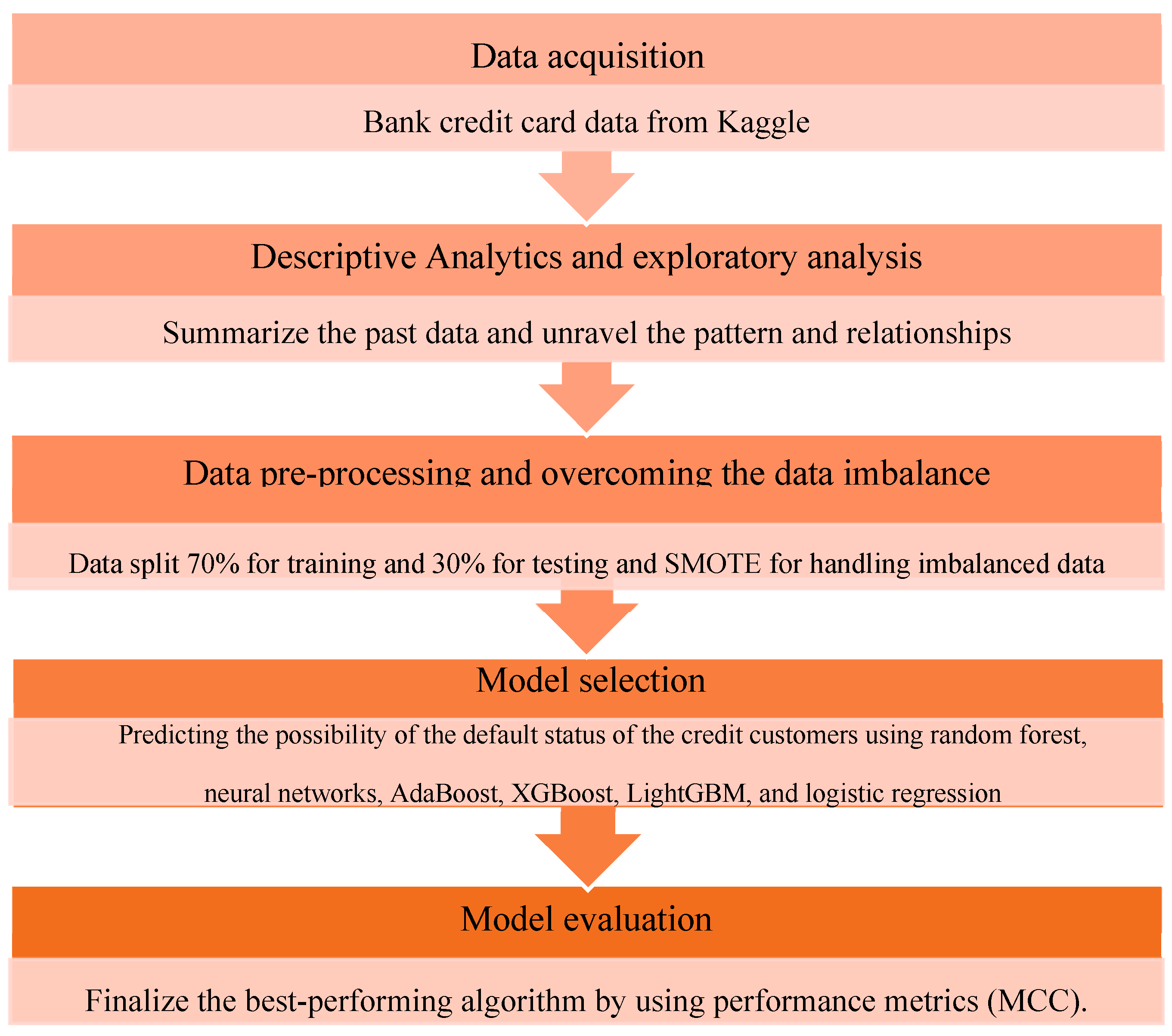
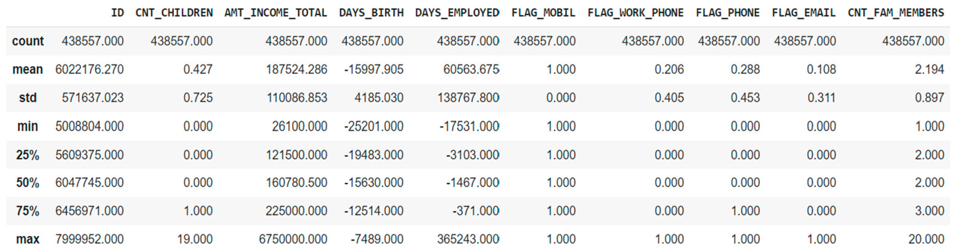
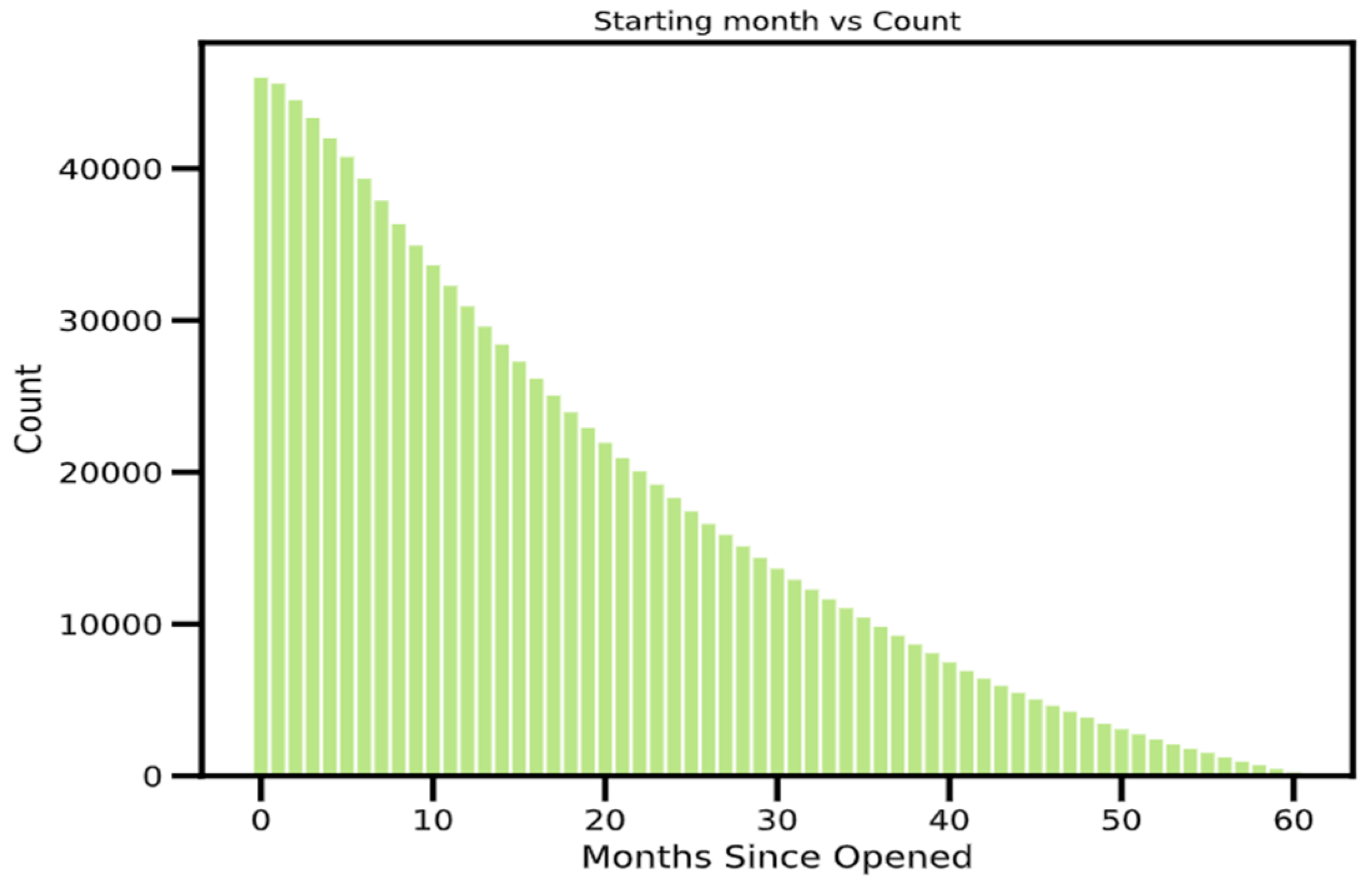
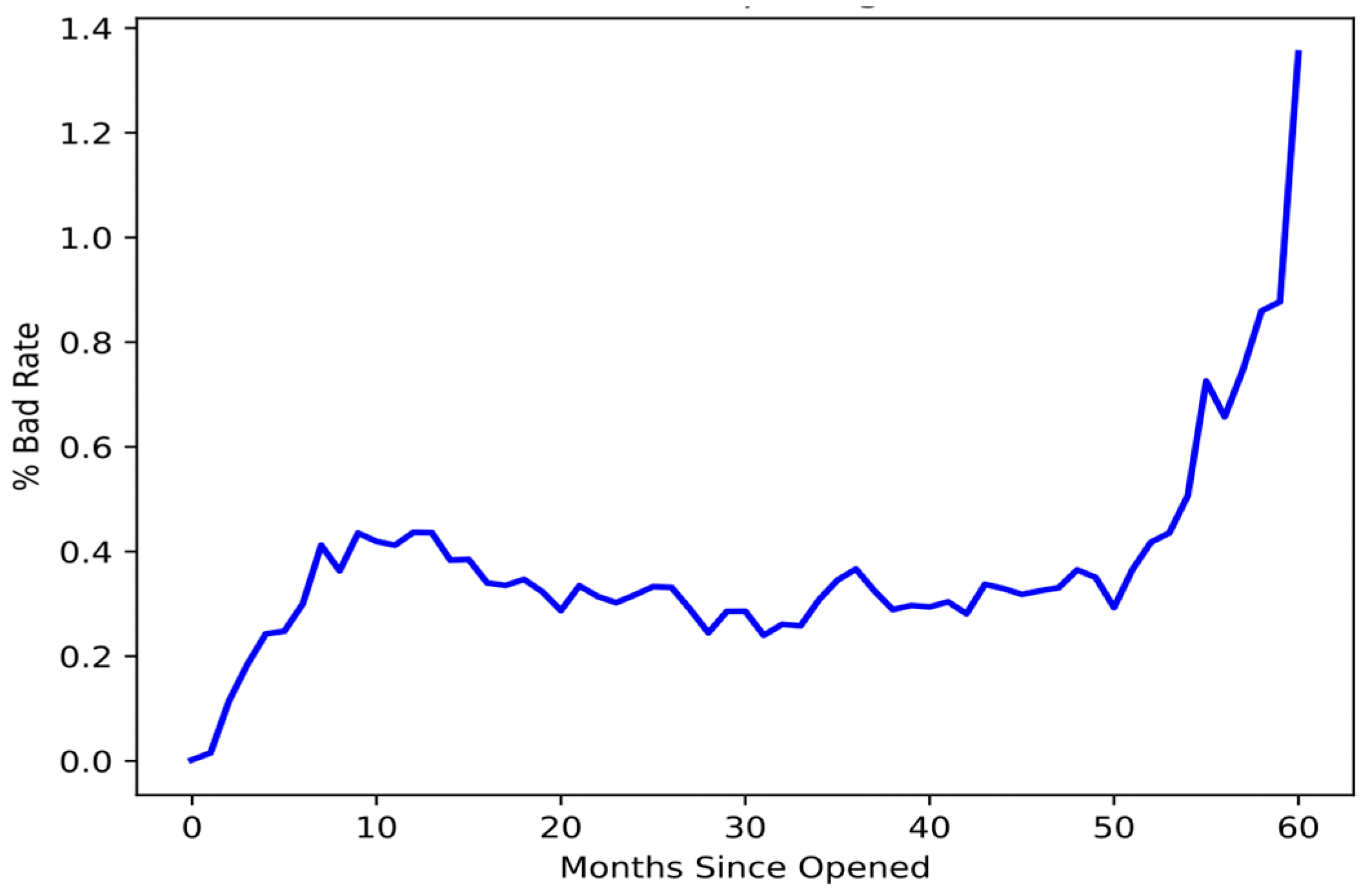
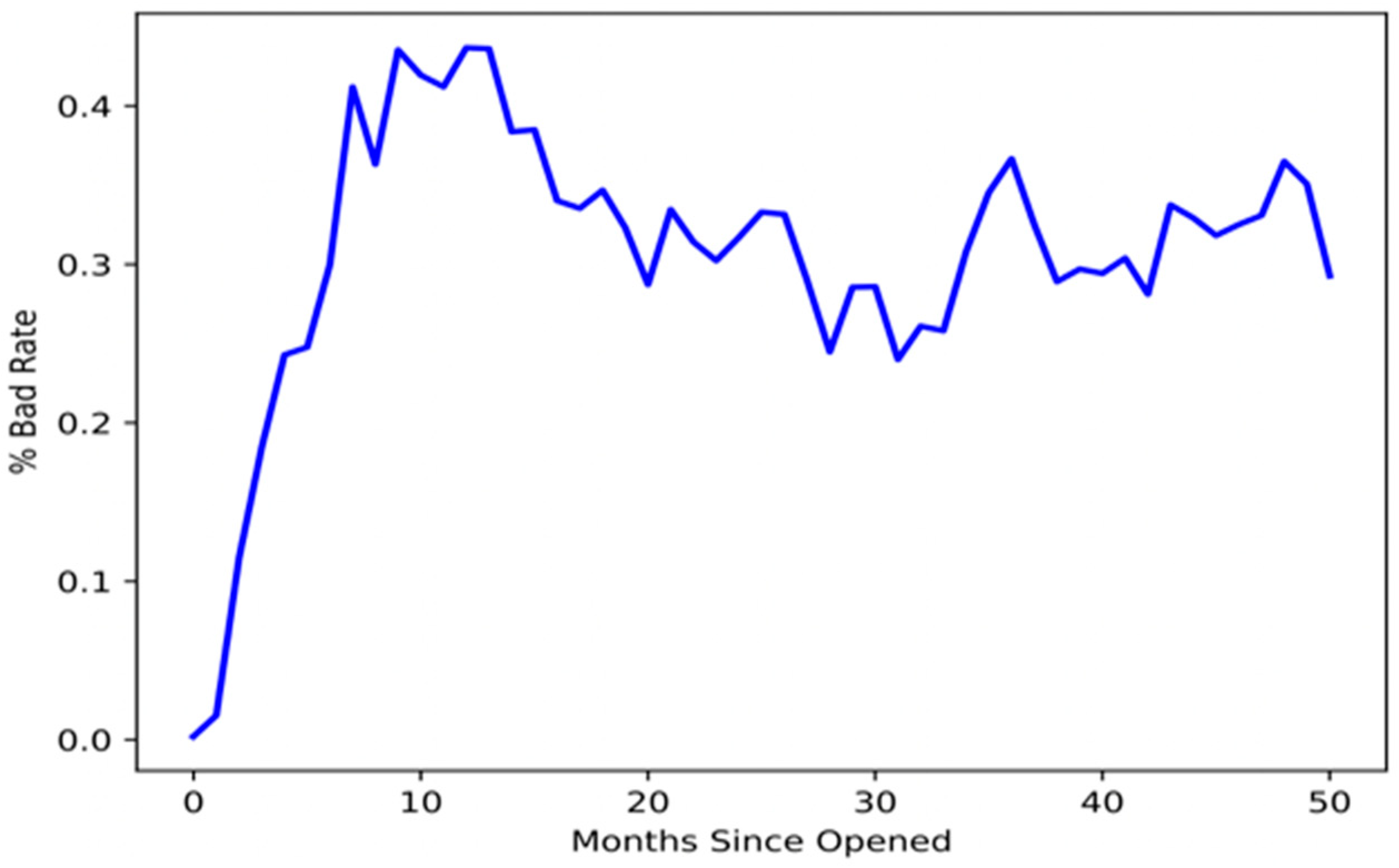
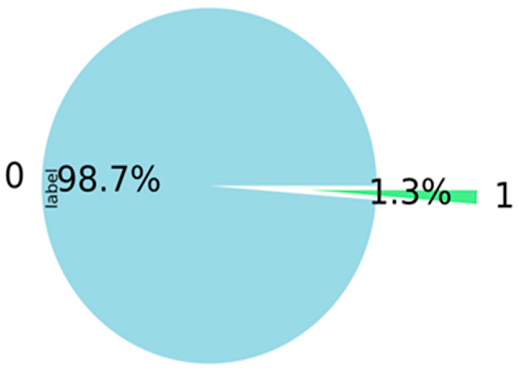
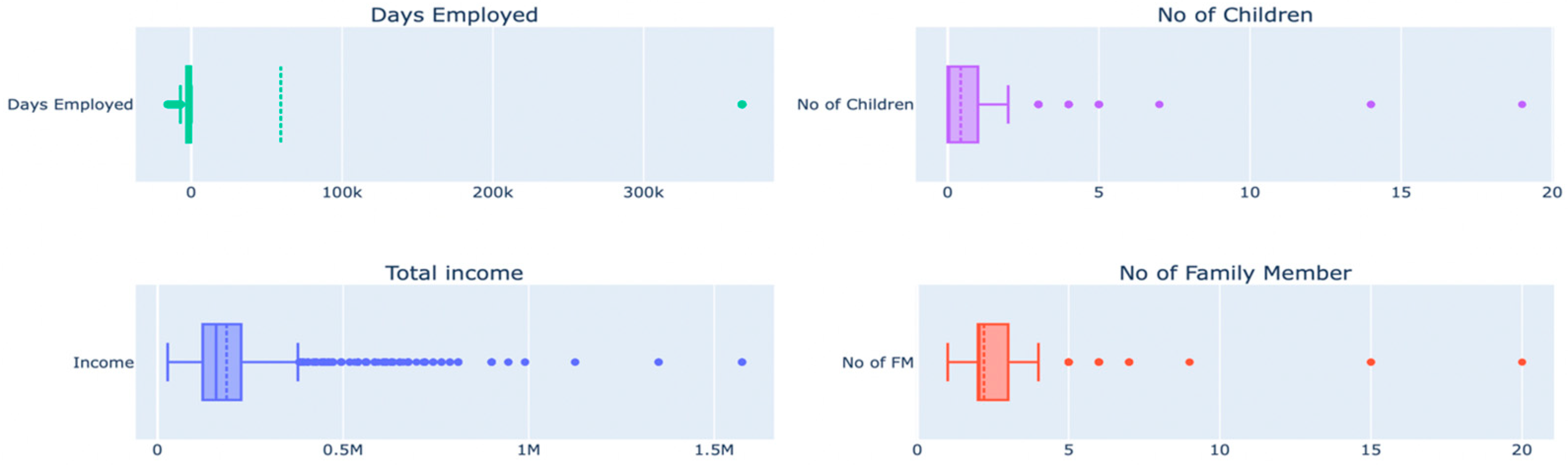


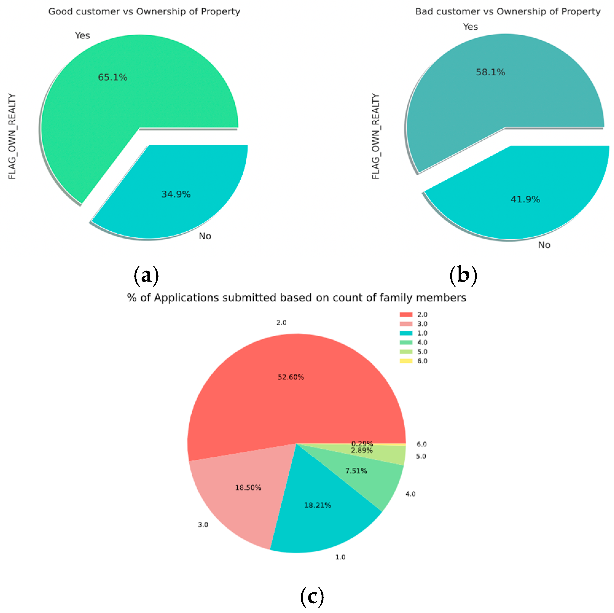


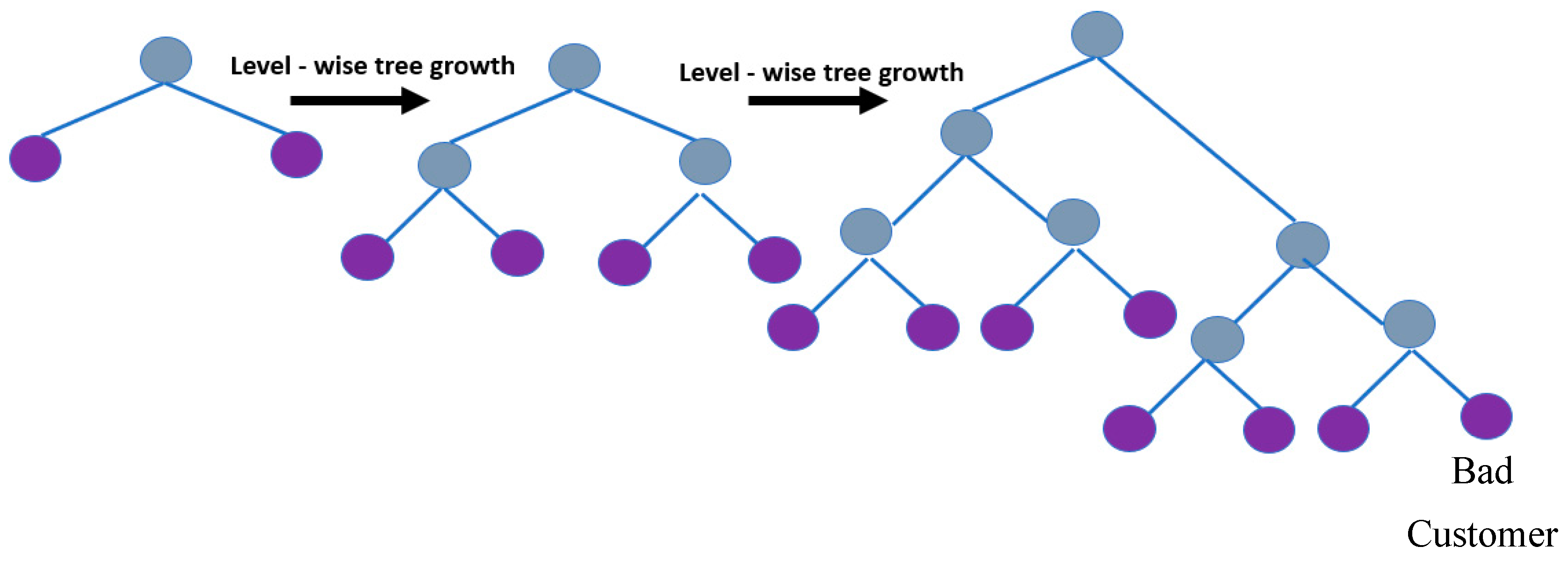
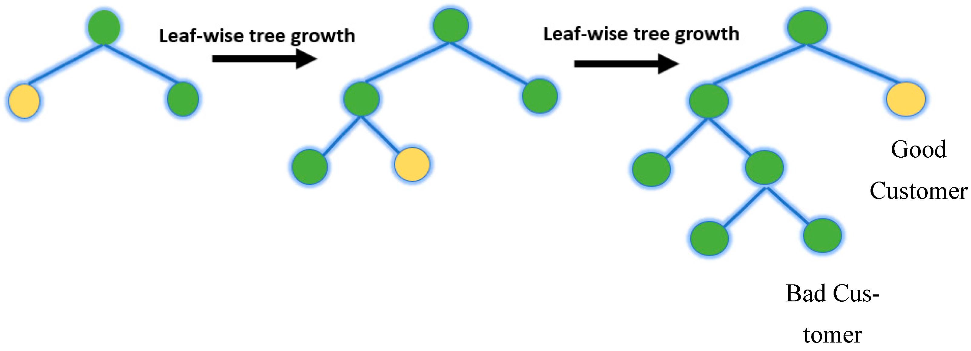
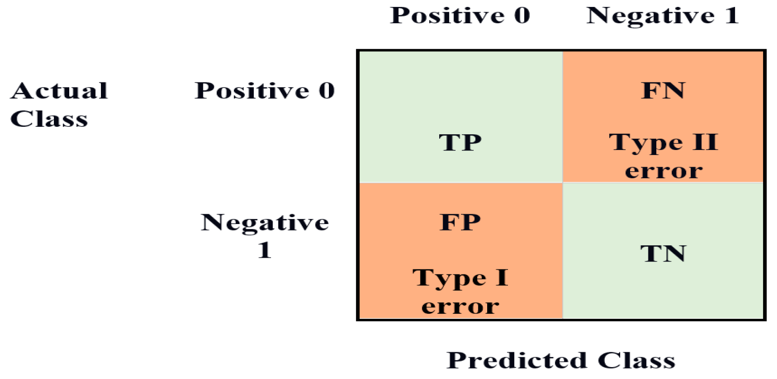


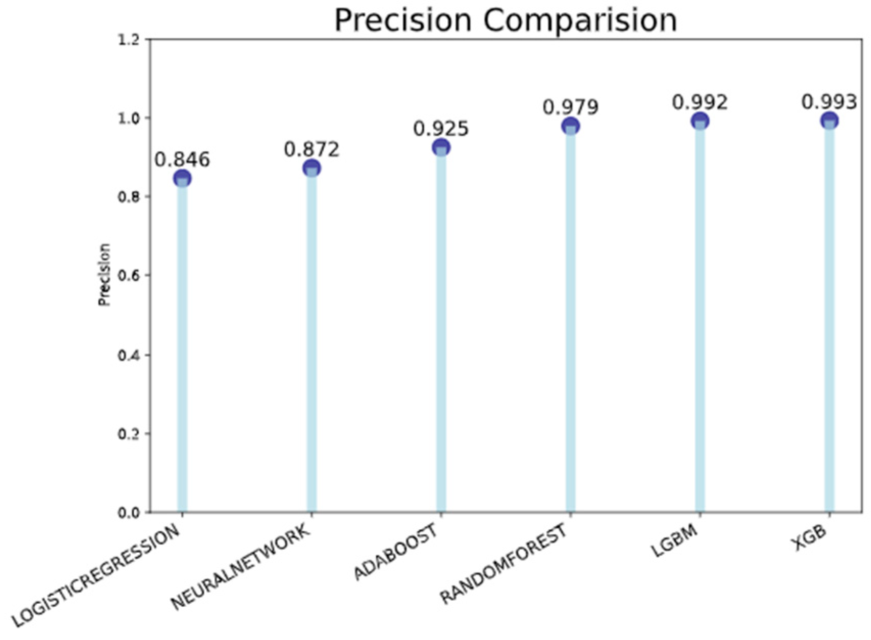
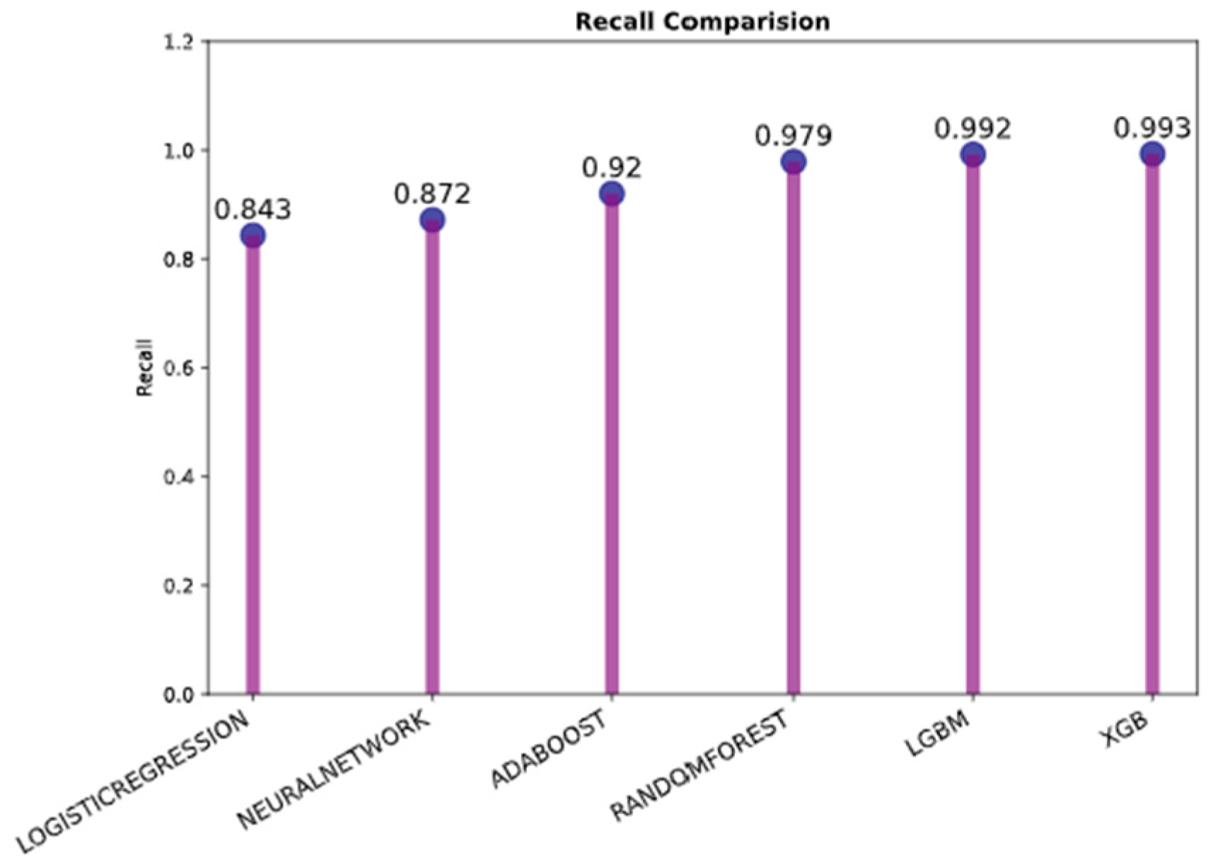
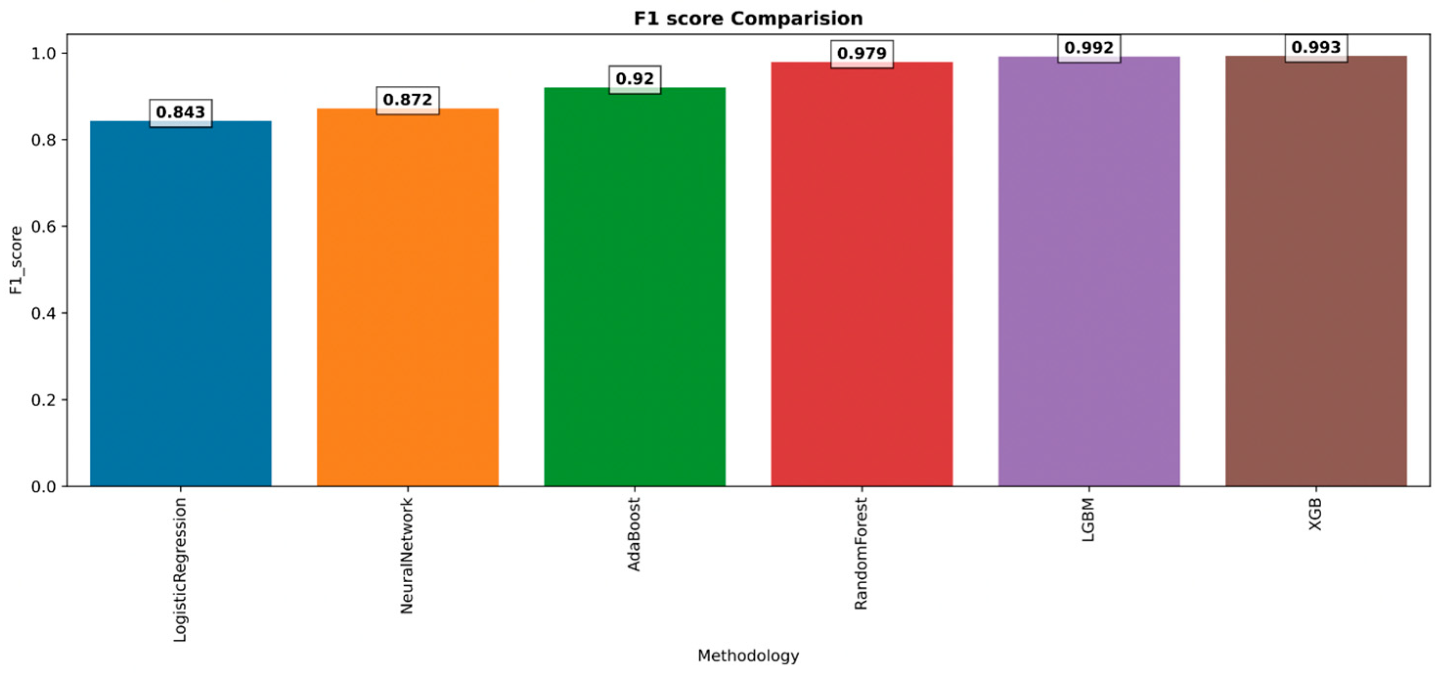

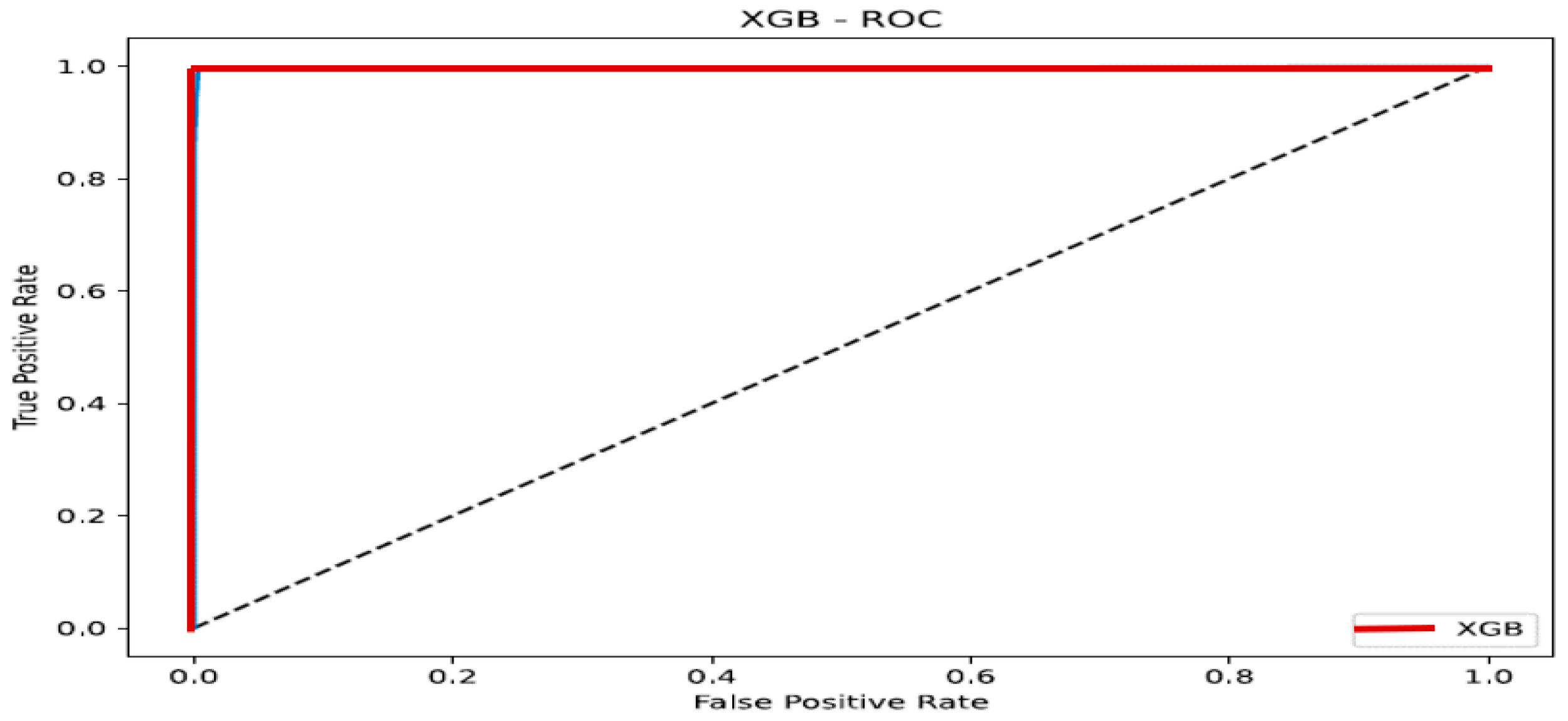


Disclaimer/Publisher’s Note: The statements, opinions and data contained in all publications are solely those of the individual author(s) and contributor(s) and not of MDPI and/or the editor(s). MDPI and/or the editor(s) disclaim responsibility for any injury to people or property resulting from any ideas, methods, instructions or products referred to in the content. |
© 2024 by the authors. Licensee MDPI, Basel, Switzerland. This article is an open access article distributed under the terms and conditions of the Creative Commons Attribution (CC BY) license (https://creativecommons.org/licenses/by/4.0/).