Quantum Computing Approach to Realistic ESG-Friendly Stock Portfolios

Abstract

Finding an optimal balance between risk and returns in investment portfolios is a central challenge in quantitative finance, often addressed through Markowitz portfolio theory (MPT). While traditional portfolio optimization is carried out in a continuous fashion, as if stocks could be bought in fractional increments, practical implementations often resort to approximations, as fractional stocks are typically not tradeable. While these approximations are effective for large investment budgets, they deteriorate as budgets decrease. To alleviate this issue, a discrete Markowitz portfolio theory (DMPT) with finite budgets and integer stock weights can be formulated, but results in a non-polynomial (NP)-hard problem. Recent progress in quantum processing units (QPUs), including quantum annealers, makes solving DMPT problems feasible. Our study explores portfolio optimization on quantum annealers, establishing a mapping between continuous and discrete Markowitz portfolio theories. We find that correctly normalized discrete portfolios converge to continuous solutions as budgets increase. Our DMPT implementation provides efficient frontier solutions, outperforming traditional rounding methods, even for moderate budgets. Responding to the demand for environmentally and socially responsible investments, we enhance our discrete portfolio optimization with ESG (environmental, social, governance) ratings for EURO STOXX 50 index stocks. We introduce a utility function incorporating ESG ratings to balance risk, return and ESG friendliness, and discuss implications for ESG-aware investors.

1. Introduction

Finding an optimal balance between risk and return of an investment is the primary goal for every investor. For investments in securities markets, this problem has been formalized by Markowitz (1952) in the sense that one needs to find optimal weights for each security, so that the portfolio maximizes the return and minimizes the risk within a given universe of considered securities. Mathematically, this amounts to minimizing the utility function $Q_c:{\mathbb{R}}^k\to \mathbb{R}$ by finding the appropriate weights $\overrightarrow{x}\in {\mathbb{R}}^k$:

$$min\left\{Q_c(\overrightarrow{r},\Sigma ,\varphi )\right\}=min\left\{\frac{\varphi }{2}{\overrightarrow{x}}^T\Sigma \overrightarrow{x}-{\overrightarrow{r}}^T\overrightarrow{x}\right\}.$$

(1)

Here, $\overrightarrow{r}$ denotes the expected returns of each portfolio component, $\varphi$ controls the level of risk-aversion and $\Sigma \in {\mathbb{R}}^{k\times k}$ is the asset price correlation matrix. The minimization is subject to the following constraints, which ensure that the entries of $\overrightarrow{x}$ can be interpreted as non-negative weights in a long-only portfolio:

$$\begin{array}{cc}\hfill & {\overrightarrow{x}}^T\overrightarrow{x}=1,\hfill \\ \hfill & x_i\ge 0i\in 1,\dots ,k.\hfill \end{array}$$

(2)

Since the correlation matrix is positive-definite and symmetric, the utility function $Q_c$ is convex, so that a solution to this optimization problem can be found in polynomial time with linear and quadratic algorithms (Kolm et al. 2014).

The vector $\overrightarrow{x}$ contains non-negative real numbers, which represent the relative weights of capital allocation to the considered assets. These weights can be multiplied by the amount of available capital to obtain the capital allocation to the respective assets. This approach faces problems when implementing such portfolios in a realistic environment, where traded contracts are discrete and security prices are finite. Hence, the theoretical capital allocation is in general not commensurate with discrete security prices. In practice, this challenge is easily overcome by rounding to the nearest multiple of the security price. The consequences for large portfolios are mild, since the relative weights of asset allocation are hardly changed by the rounding. For small and intermediate portfolios, this rounding may affect the relative weighting significantly and create sub-optimal implementations of originally optimal portfolios.

Discrete extensions of the Markowitz portfolio optimization, where the discreteness of securities contracts is considered from the start, have been studied for a long time, because such discrete portfolios also facilitate the inclusion of further realistic features such as transaction costs or Boolean constraints on stock selection (Mugel et al. 2022; Rubio-García et al. 2022; Young 1998). Intensive studies have been conducted on the problem of transaction costs and the optimal investment trajectory in a multi-period setting. These studies revealed that the discrete Markowitz portfolio theory (DMPT) is a non-polynomial hard problem (Bonami and Lejeune 2009; Coleman et al. 2006; Jobst et al. 2001; Kellerer et al. 2000; Mansini and Speranza 1999), even if the trajectory problem is only formulated for a single period (Rosenberg et al. 2016).

The main problem is that the number of possible portfolio compositions grows factorially with the number of assets in the investment universe and the allowed number of assets in the portfolio. If our portfolio may contain n not necessarily different lots out of an investment universe of k different assets, where each asset can be bought multiple times, the total number of possible portfolio combinations is given by a binomial coefficient:

$$M=\left(\genfrac{}{}{0pt}{}{n+k-1}{k}\right)=\frac{(n+k-1)!}{k!(n-1)!}.$$

(3)

For a moderate portfolio size of $n=1000$ and a small investment universe of $k=4$ stocks, the number of possible portfolios is already $M>{10}^{10}$. If we extend the number of considered stocks to $k=50$ and keep $n=1000$, the number of possible portfolios grows to $M>{10}^{86}$, which is larger than current estimates of the number of atoms in the entire universe. At the same time, there is no efficient algorithm for finding the optimal combination out of these M combinations on a classical computer, so that only a brute force approach guarantees success. However, most realistic problems are too large to be solved by testing each of the M combinations, so finding the exact solution of large problems is not feasible on classical machines. Therefore, these problems have been approached using heuristic and approximate methods on classical computers, which do not guarantee an optimal solution (Castro et al. 2011; Li and Tsai 2008; Mansini and Speranza 1999; Streichert et al. 2004; Vielma et al. 2008).

In recent years, the rapid progress in manufacturing of quantum processing units (QPUs) and the development of hybrid quantum-classical workflows, not only for universal quantum computers (Abrams and Lloyd 1998; Brandhofer et al. 2022; Chen et al. 2023; Farhi et al. 2014; Zheng 2021), but also for quantum annealers (Cohen et al. 2020a, 2020b; Elsokkary et al. 2017; Grant et al. 2021; Jacquier et al. 2022; Orús et al. 2019; Palmer et al. 2022; Phillipson and Bhatia 2021; Romero et al. 2023), has reignited interest in this type of problem. Meanwhile, quantum annealers have been shown to provide a quantum advantage for certain classically intractable problems (King et al. 2023) and seem to provide a promising platform for solving quadratic binary optimization and integer quadratic optimization, even in the presence of hard and weak constraints. Based on these prospects, portfolio optimization is a natural application for quantum computing in finance, and in particular quantum annealers. For a broader review of quantum computing applications in finance, see refs. (Herman et al. 2023; Jacquier et al. 2022; Orús et al. 2019).

Recently, awareness of environmental, social and governance (ESG) aspects of investing has grown among private and institutional investors alike. A growing number of financial products caters to the growing demand and incorporates ESG aspects into the product design. The trend toward more ESG awareness is likely to get further amplified by regulatory updates on international and national levels. See, for example, Bruno and Lagasio (2021) for an overview of ESG regulation in the banking sector across Europe. In January 2023, European authorities agreed on a European implementation of the internationally developed Basel III update that will result in an updated capital requirement regulation (CRR) and capital requirement directive (CRD), including requirements on ESG awareness and inclusion in risk management. Up to now, integrating ESG constraints in investment decisions has been up to individual preference, but it can be expected to become a required standard in the near future in the EU. The inclusion of ESG risk as an additional risk factor besides historical covariance into the Markowitz framework (see Equation (1)) is actively being investigated (Chen et al. 2021; López Prol and Kim 2022; Pedersen et al. 2021; Utz et al. 2014).

Meanwhile, ESG data in different formats are available from a number of data providers such as MSCI, ISS ESG, Refinitiv, Sustainalytics, and others. The approach for establishing ESG ratings varies. Some providers offer ESG ratings or scores that aim to capture investment risks by assessing how effectively a company manages ESG risks in its business (”financial”). Other providers aim to characterize the impact of a corporation on the environmental, social and governance dimensions, with the goal of facilitating informed decisions for investors (“impact”). The ISS ESG data used in this analysis capture both the financial and impact aspects of ESG ratings. The scores can be given on the level of environmental, social and governance dimensions, with focus on smaller sub-areas, or as a single aggregate score on a company level, which seeks to represent the average of all relevant aspects. For a critical review of available data sets and methodologies, see refs. (Berg et al. 2022; Larcker et al. 2022).

How ESG ratings should be best included into the Markowitz framework is an open question. Both inclusion of the expected ESG score into the vector of expected returns (Alessandrini and Jondeau 2021; Lauria et al. 2022; Shushi 2022; Varmaz et al. 2022) and optimizing the ESG score in the form of a multi-objective optimization (Cesarone et al. 2022; De Spiegeleer et al. 2023; Hirschberger et al. 2013; Utz et al. 2014) have been investigated in the literature. Including the ESG score into the returns vector is intrinsically ambiguous, since it compares the ESG score and monetary returns as if these quantities had the same units. This introduces a conversion law between returns and ESG scores, which depends on the exact form of the ESG score data, which may differ between various providers. However, it would be preferable to have a unique framework for incorporating ESG scores into the Markowitz utility function (see Equation (1)). The multi-objective optimization approach, on the other hand, may be unable to control the interplay between returns, variance and ESG performance, depending on the exact implementation.

In this work, we extend the Markowitz portfolio theory to include the ESG scores directly in the utility function in a way that avoids the ambiguity in relation to the returns. Furthermore, we can investigate and control the interplay between returns, variance and ESG performance. Our formulation is applicable to standard (continuous) and also discrete mean-variance (Markowitz) portfolio optimization, allowing for application in realistic scenarios. We demonstrate the feasibility of our method on classical computers for the continuous case and on quantum annealers for the discrete portfolio optimization case. The results are based on real market data of selected stocks from the EURO STOXX 50 index, as well as actual respective ESG scores from ISS ESG.

The paper is divided as follows: Section 2 contains the main results of our study. In Section 2.1, we establish the correct normalization approach for the discrete Markowitz problem, so that solutions for the continuous and the discrete formulation may be compared. We provide a relationship between the total number of stocks in the portfolio and the risk-aversion parameter, which needs to be considered. In Section 2.2, we introduce a budget constraint into the discrete portfolio problem, so that realistic scenarios with limited budgets may be investigated. We compare the usual rounding approach to a direct search of discrete optimal portfolios and find that rounding produces sub-optimal portfolios for small to medium investment budgets. In Section 2.3, we introduce a novel framework for including ESG scores into both continuous and discrete Markowitz portfolio optimization, which is applicable even to ESG data with heterogeneous scales. In Section 3, we discuss our results and potential implications for ESG-aware investors. Finally, in Section 4, we summarize our results and provide an outlook on future research topics.

2. Results

2.1. Discrete Markowitz Portfolio Theory and the Role of the Risk-Aversion Parameter

Here, we investigate the connection between the continuous and the discrete Markowitz portfolio theory. Naively, one could expect that the discrete approach should yield the same results as the continuous version for large portfolios, where the discreteness becomes less relevant. As mentioned in the introduction, the single period DMPT is already an NP-hard problem (Castro et al. 2011; Rosenberg et al. 2016).

To explore this connection in detail, we formalize the DMPT problem with a fixed number of stocks in the portfolio in the following way:

$$min\left\{Q_d(\overrightarrow{r},\Sigma ,\varphi ,N_{\mathrm{tot}})\right\}=min\left\{\frac{\varphi }{2}{\overrightarrow{x}}^T\Sigma \overrightarrow{x}-{\overrightarrow{r}}^T\overrightarrow{x}\right\}.$$

(4)

The crucial difference with the continuous case (see Equation (1)) lies in the discrete nature of the constraints:

$$\begin{array}{cc}\hfill & \overrightarrow{x}=(x_1,\cdots ,x_k)\mathrm{with}{x}_i\in \mathbb{N}\forall i,\hfill \\ \hfill & \sum _{i=1}^k{x}_i=N_{\mathrm{tot}}.\hfill \end{array}$$

(5)

Note that the return vector $\overrightarrow{r}$ and the covariance matrix $\Sigma$ do not change their meaning, since these quantities are dimensionless. Therefore, no special care has to be taken when interpreting the return vector $\overrightarrow{r}$ or covariance matrix $\Sigma$ in the continuous vs. the discrete case.

If the raw solution of this naive approach (Equations (4) and (5)) is denoted as ${\overrightarrow{X}}_{\mathrm{naive}}$, we can calculate the relative portfolio weights ${\overrightarrow{x}}_{d,\mathrm{naive}}$, which may be compared to the solution ${\overrightarrow{x}}_c$ from the continuous case, by dividing through the portfolio size $N_{\mathrm{tot}}$:

$${\overrightarrow{x}}_{d,\mathrm{naive}}=\frac{{\overrightarrow{X}}_{\mathrm{naive}}}{N_{\mathrm{tot}}}.$$

(6)

If we calculate the Euclidean distance between the continuous solution ${\overrightarrow{x}}_c$ and these naive weights from Equation (6), we would expect the difference from ${\overrightarrow{x}}_c$ to vanish with increasing $N_{\mathrm{tot}}$:

$$\underset{N_{\mathrm{tot}}\to \infty }{lim}\left|\right|{\overrightarrow{x}}_c-{\overrightarrow{x}}_{d,\mathrm{naive}}{\left|\right|}_2=0.$$

(7)

We calculated this difference with the formalism described so far. The continuous solution was extracted using the CVXPY (Agrawal et al. 2018; Diamond and Boyd 2016) software package for the Python programming language. For solving the discrete portfolio optimization problem, one could use a heuristic classical algorithm (García et al. 2022), an algorithm for gate-based quantum computers (Mugel et al. 2022; Shunza et al. 2023), a quantum-inspired approximate algorithm for classical computers (Mugel et al. 2022) or a quantum annealer (Jacquier et al. 2022; Sakuler et al. 2023). For an overview of the use of various computing approaches in portfolio optimization, see Buonaiuto et al. (2023).

D-Wave quantum annealers implement the Ising model, known from theoretical physics, in a specialized quantum processing unit. These annealers are not universal quantum computers. Therefore, their applicability is limited to problems which can be represented in terms of the Ising model (Lucas 2014). The solution of the optimization problem is extracted via a physical annealing process, which gradually cools the quantum processing unit down to temperatures close to absolute zero. Subsequently, the quantum state of the system is measured and translated back to the original problem space.

We have decided to use a quantum annealer because the discrete portfolio optimization problem can be rewritten as an Ising model (Jacquier et al. 2022; Lucas 2014). Therefore, the quantum annealer is a natural choice when solving discrete portfolio problems. Other previously mentioned approaches are also viable (Buonaiuto et al. 2023), but either cannot reach the problem sizes considered here or have no guarantee of providing an optimal solution. Nevertheless, heuristic approaches may yield very good results, as demonstrated by García et al. (2022).

The Ising model is formulated in terms of discrete variables, which represent magnetic moments. These can be in one of two quantum states $s_i\in \{+1,-1\}$. A simple transformation allows us to convert these magnetic moments into zeros and ones $a_i\in \{0,1\}$, which can be used to represent integer numbers in binary encoding:

$$a_i=\frac{s_i+1}{2}$$

(8)

This transformation between integer optimization problems and the Ising model is well known (Lucas 2014) and automatically carried out in various software packages like D-Wave Ocean.1 The optimization problem can be entered into Ocean in a declarative way using a domain-specific language. In particular, this means that no imperatively formulated solution algorithm is required. This software package also handles the transformation of constraints into penalty terms in a proprietary way. For details on the technical implementation of D-Wave solvers, see D-Wave Systems Inc. (2021). Note, however, that going beyond long-only portfolios would require a type of optimization constraint that is currently not supported by D-Wave software packages.

Now, we estimate a theoretical upper bound to the number of qubits required by our approach. Since D-Wave Ocean uses binary encoding for integer variables, the upper bound for the required number of qubits $N_{\mathrm{qubit}}$ scales with the logarithm of the portfolio size $N_{\mathrm{tot}}$ and linearly with the number of assets k within our investment universe:

$$N_{\mathrm{qubit}}\le k·\left({log}_2\left(N_{\mathrm{tot}}+1\right)+1\right).$$

(9)

Of course, the proprietary algorithm of D-Wave may require an overhead of additional qubits to encode the problem on real-world hardware. Unfortunately, these details are not public and cannot be investigated here further.

The results of our calculations using CVXPY for the continuous problem and D-Wave Ocean for the discrete problem are shown in Figure 1a. We realized that the difference in Equation (7) does not converge to zero with the growing portfolio size. This is the case because risk-aversion parameters for the continuous and discrete portfolio cases are not directly comparable. This phenomenon does not depend on the exact value of $\varphi >0$.

If we view the continuous problem of Equation (1) as a particular discrete problem, in which the solution vector $\overrightarrow{x}$ is rescaled by $1/N_{\mathrm{tot}}$ and the limit $N_{\mathrm{tot}}\to \infty$ is applied, we can write it in the following way:

$$\begin{array}{cc}\hfill min\left\{Q_c(\overrightarrow{r},\Sigma ,\varphi )\right\}& =min\left\{\underset{N_{\mathrm{tot}}\to \infty }{lim}\left(\frac{\varphi }{2}\frac{{\overrightarrow{x}}^T\Sigma \overrightarrow{x}}{N_{\mathrm{tot}}^2}-\frac{{\overrightarrow{r}}^T\overrightarrow{x}}{N_{\mathrm{tot}}}\right)\right\}\hfill \\ \hfill & =min\left\{\underset{N_{\mathrm{tot}}\to \infty }{lim}\left(\frac{1}{N_{\mathrm{tot}}}\right)\left(\left(\frac{1}{N_{\mathrm{tot}}}\right)\frac{\varphi }{2}{\overrightarrow{x}}^T\Sigma \overrightarrow{x}-{\overrightarrow{r}}^T\overrightarrow{x}\right)\right\}.\hfill \end{array}$$

(10)

The constraints are the same as in Equation (5). It is clear that the discrete problem of Equation (10) can only converge to the continuous problem of Equation (1) if the additional factor of $1/N_{\mathrm{tot}}$ in front of the covariance term is absorbed into the risk-aversion parameter. Hence, the risk-aversion parameter of the discrete case ${\varphi }_d$ is connected to the risk-aversion parameter of the continuous case ${\varphi }_c$ in the following way:

$${\varphi }_d=\frac{{\varphi }_c}{N_{\mathrm{tot}}}.$$

(11)

Therefore, we need to respect the mapping for the normalized risk-aversion parameter $\varphi$ in Equation (11) if we want to compare portfolios from continuous and discrete optimization. Doing this correctly and re-calculating the difference in Equation (7) with the normalized risk-aversion parameter, one obtains the second curve in Figure 1a, which clearly converges to zero for a large number of stocks $N_{\mathrm{tot}}$.

It is also instructive to examine the solutions of the naive approach for different portfolio sizes (without renormalizing $\varphi$) and their position in volatility–return space. This is shown in Figure 2. All solutions lie on the ‘efficient frontier’, as the surface of the maximum return as a function of volatility is commonly called. This efficient frontier in the background was generated by sampling random portfolio compositions.

As we can see, the solutions from the naive discrete approach trend towards the minimum-variance solution if we naively fix $\varphi =1$. The reason is clear from Equation (11): with $N_{\mathrm{tot}}\gg 1$, we should have adapted the risk-aversion parameter to the portfolio size. For example, we should have used $\varphi =1/1000$ for $N_{\mathrm{tot}}=1000$ in order to obtain comparable solutions. Fixing $\varphi =1$ irrespective of the portfolio size leads to portfolios for which risk aversion becomes increasingly important as the size of the portfolio grows. Therefore, the naive approach always converges to the minimum-variance portfolio for $N_{\mathrm{tot}}\gg 1$. Also note how the scale of variations in volatility in Figure 2 is already small for $N_{\mathrm{tot}}=10$ due to the overemphasis on risk aversion. The convergence to the minimum variance portfolio occurs rapidly as a function of the number of stocks $N_{\mathrm{tot}}$. At $N_{\mathrm{tot}}=1000$, the composition is already practically indistinguishable from the minimum variance portfolio.

As a final test, we carried out another calculation, in which we have neglected the term related to maximizing the return in the utility function (see Equation (4)). If only the covariance term is considered, the optimization should always yield the minimum-variance portfolio irrespective of the portfolio size. This is clearly the case, as shown in Figure 1b. The remaining difference in portfolio compositions between the continuous and discrete solutions is purely due to the discrete stock allocation in the latter case. Thus, we have shown that renormalizing the risk-aversion parameter $\varphi$ according to Equation (11) is crucial.

Now that we have established a discrete portfolio optimization approach, which is comparable to the well-known continuous approach, we introduce budget constraints in the following subsection to mimic realistic portfolio selection problems.

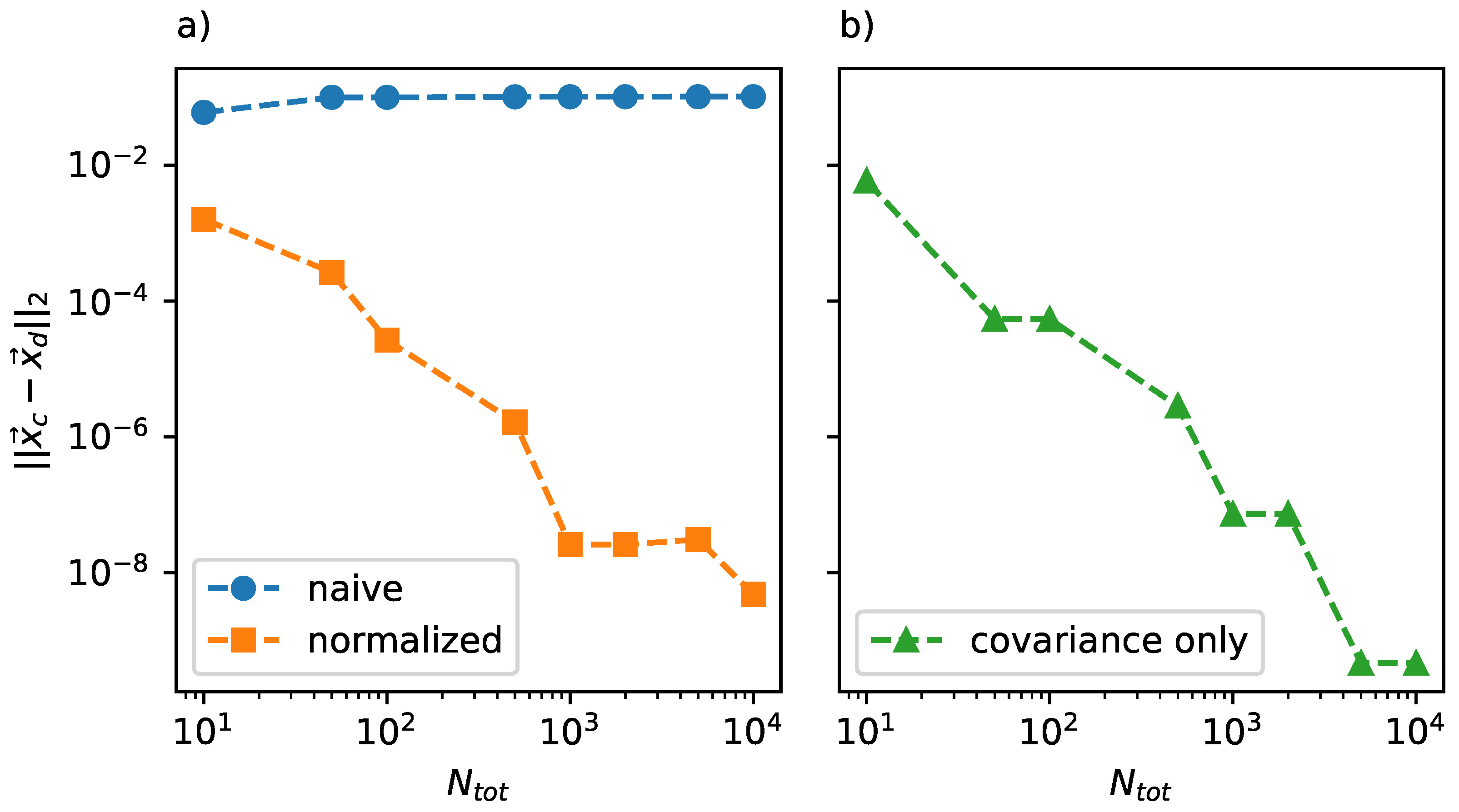
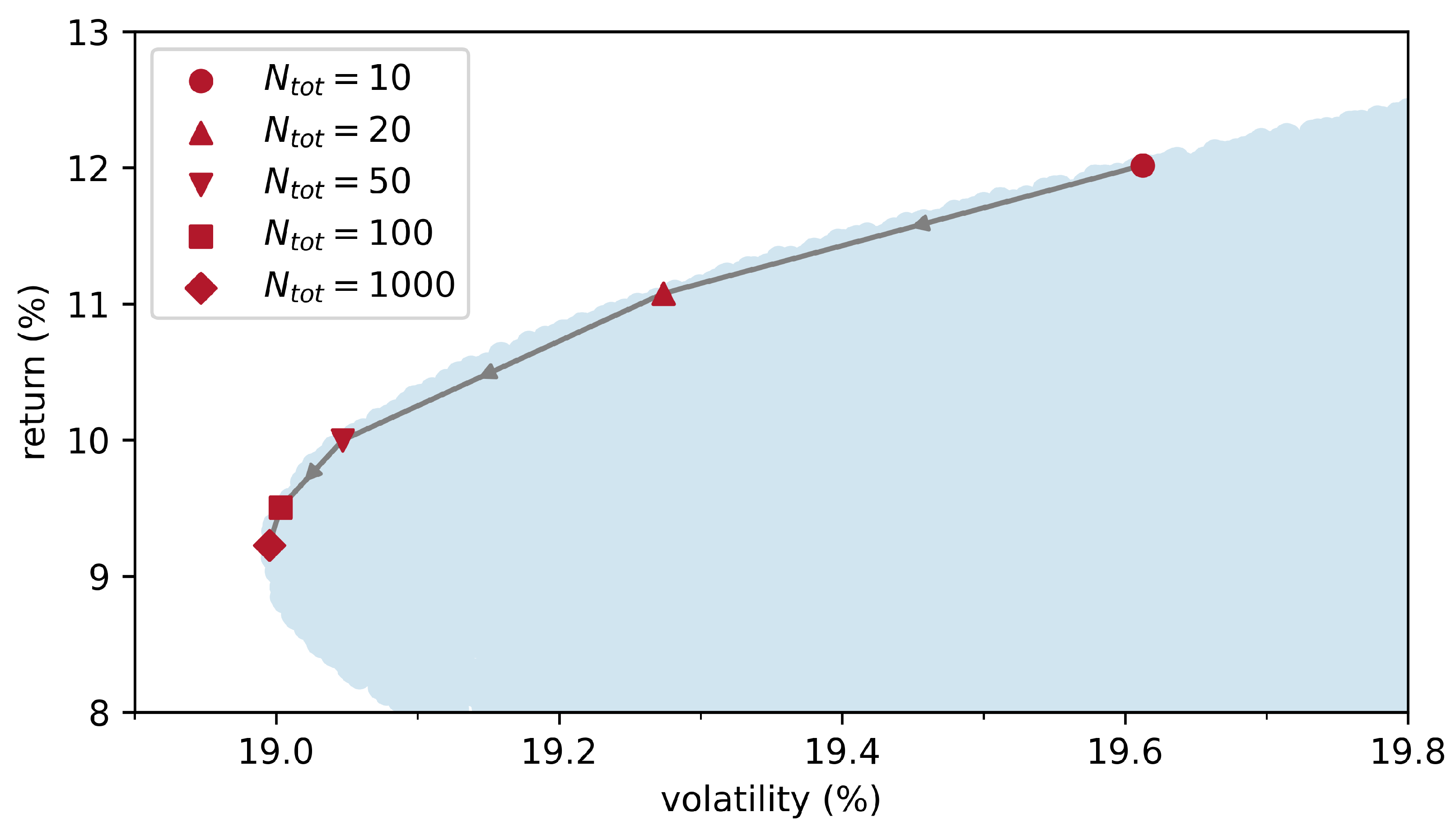
2.2. Discrete Markowitz Portfolio Theory with a Limited Investment Budget

To now, we have only solved the portfolio problem with a limited number of stocks. In practice, the number of stocks that can be purchased is usually not directly limited but indirectly limited via the total available investment budget. To make our study more realistic, we now fix the total available investment budget. This means that the algorithm will not optimize different stocks like for like, but rather optimize portfolios with many low-price stocks versus portfolios with few high-price stocks.

As explained in Section 2.1, the total number of stocks in discrete Markowitz portfolio theory plays a crucial role in the risk-aversion parameter, which determines the compromise between risk and return of the portfolio. With the risk-aversion parameter for the continuous portfolio ${\varphi }_c$, we write the utility function for the discrete portfolio theory in the following way:

$$Q_d(\overrightarrow{r},\Sigma ,{\varphi }_c,N_{\mathrm{tot}})=\frac{{\varphi }_c}{2N_{\mathrm{tot}}}{\overrightarrow{x}}^T\Sigma \overrightarrow{x}-{\overrightarrow{r}}^T\overrightarrow{x}.$$

(12)

The minimization of this utility function is subject to the following constraints:

$$\begin{array}{cc}\hfill & \overrightarrow{x}=(x_1,\cdots ,x_k)\mathrm{with}{x}_i\in \mathbb{N}\forall i,\hfill \\ \hfill & \sum _{i=1}^k{x}_i=N_{\mathrm{tot}},\hfill \\ \hfill & {\overrightarrow{p}}^T\overrightarrow{x}-B\le 0.\hfill \end{array}$$

(13)

Here, $\overrightarrow{p}$ is the vector which contains the price per stock for each stock. Therefore, ${\overrightarrow{p}}^T\overrightarrow{x}$ is the initial value of the portfolio. B is the initially available investment budget. In this sense, we constrain the optimization to the space of portfolios that can be purchased with the initially available budget. Since we also maximize return via the utility function (Equation (12)), the algorithm will yield portfolios which use the available budget to the maximum extent.

In practice, we will study the problem defined by Equations (12) and (13) at a fixed number of stocks $N_{\mathrm{tot}}$. If the number of stocks $N_{\mathrm{tot}}$ is chosen as too small, the initial portfolio value will be far below the initial budget B. If we choose a too large number for $N_{\mathrm{tot}}$, the number of possible portfolio combinations will exceed the capabilities of contemporary quantum hardware. Therefore, we start with low $N_{\mathrm{tot}}$ and gradually increase this number until the difference between portfolio value and available budget ${\overrightarrow{p}}^T\overrightarrow{x}-B$ becomes sufficiently small. As we will see, this approach yields good results even in realistic settings.

Of course, we would like to compare these discrete solutions to portfolios that are based on the usual continuous Markowitz theory. In the continuous case, the solution ${\overrightarrow{x}}_c$ provides a relative allocation of the available investment budget to the respective stocks. The actual portfolio is then usually constructed by multiplying the relative weights ${\overrightarrow{x}}_c$ by the available budget B. This gives the budget which is allocated to each stock. To obtain the integer number of stocks that has to be bought for each sort, one divides by the price of the respective stock and rounds to the next integer, which is denoted as $\lfloor \rceil$. Therefore, we can write the integer portfolio composition based on the rounding approach as:

$${\left({\overrightarrow{x}}_{c,r}\right)}_i=⌊\frac{B·{\left({\overrightarrow{x}}_c\right)}_i}{p_i}⌉.$$

(14)

Here, ${\left({\overrightarrow{x}}_c\right)}_i$ is the i-th component of the vector of relative allocation from the continuous Markowitz theory and $p_i$ is the price of the i-th stock. Interestingly, the rounding approach according to Equation (14) yields portfolio compositions, which are substantially different from the discrete approach using Equations (12) and (13), even if consistent values for the risk-aversion parameter ${\varphi }_c$ are used. Remember that these two approaches only coincide in the limit of an infinite available budget, as explained in Section 2.1.

We have carried out continuous and discrete portfolio optimization with a risk-aversion parameter of ${\varphi }_c=8$ and a total investment budget of B = EUR 100,000. For simplicity, the investment universe is again limited to BMW (ISIN DE0005190003), Deutsche Post (ISIN DE0005552004), Deutsche Telekom (ISIN DE0005557508) and Infineon (ISIN DE0006231004). In the discrete case, we have used $N_{\mathrm{tot}}=3401$, which produces an initial portfolio value of ${\overrightarrow{p}}^T{\overrightarrow{x}}_d$ = EUR 99,999.87 for the optimal solution. The rounding approach (see Equation (14)) may of course slightly violate the budget constraint. Thus, the rounded solution yields an initial portfolio value of ${\overrightarrow{p}}^T{\overrightarrow{x}}_{c,r}$ = EUR 100,006.32 and a total number of stocks of $N_{\mathrm{tot}}=4026$. A larger number of stocks for the rounded continuous case appears because the standard Markowitz approach puts a large relative weight on Deutsche Telekom, which has the lowest Euro value per stock within the considered investment universe. This means that a larger number of these stocks will be bought with the available budget.

The resulting portfolio compositions for the discrete and rounded continuous cases are shown in Figure 3, both in terms of the number of stocks bought per ISIN and the invested budget per ISIN. We observe that the respective portfolio compositions are strikingly different. The rounded continuous approach yields a solution which is well diversified in terms of the allocated budget. The discrete approach, on the other hand, yields a portfolio which is slightly more concentrated in terms of budget allocation. This effect is likely due to the strict budget constraint in the discrete case, which forces the optimization to pick allocations that fit the specific budget constraints.

We also investigated the position of the obtained portfolios in the volatility–return space (see Figure 4). The discrete solution is right at the efficient frontier, i.e., it yields an optimal return for the given volatility. The rounded continuous portfolio has a lower volatility, but also yields a significantly lower than optimal return. The deviation of nearly two percentage points in return is larger than one may expect from the seemingly harmless rounding approach. The effects of the rounding observed here are likely relevant in practical applications. In fact, one can expect even larger deviations for portfolios with a larger number of components.

Our results clearly show that the continuous and discrete approaches only converge to identical results in the limit of an infinite portfolio size. For a limited investment budget, the approach of minimizing the utility function for the discrete case directly on a quantum computer yields results which are far superior to the widely used rounding method based on the standard Markowitz approach, even for moderately sized portfolios and a limited investment universe. We expect that the quantum computing approach will have even stronger appeal for large investment universes, since the discreteness of individual components will play an even more important role there.

Now that we have established the superiority of the quantum computing approach in the case of a limited budget, we come to the main idea of our study: the inclusion of ESG data into the discrete portfolio optimization problem.

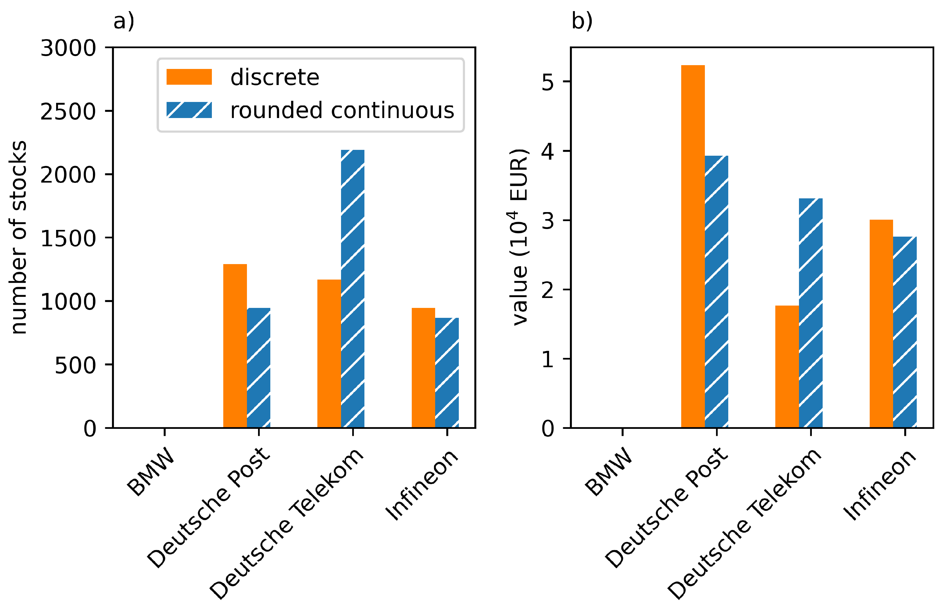
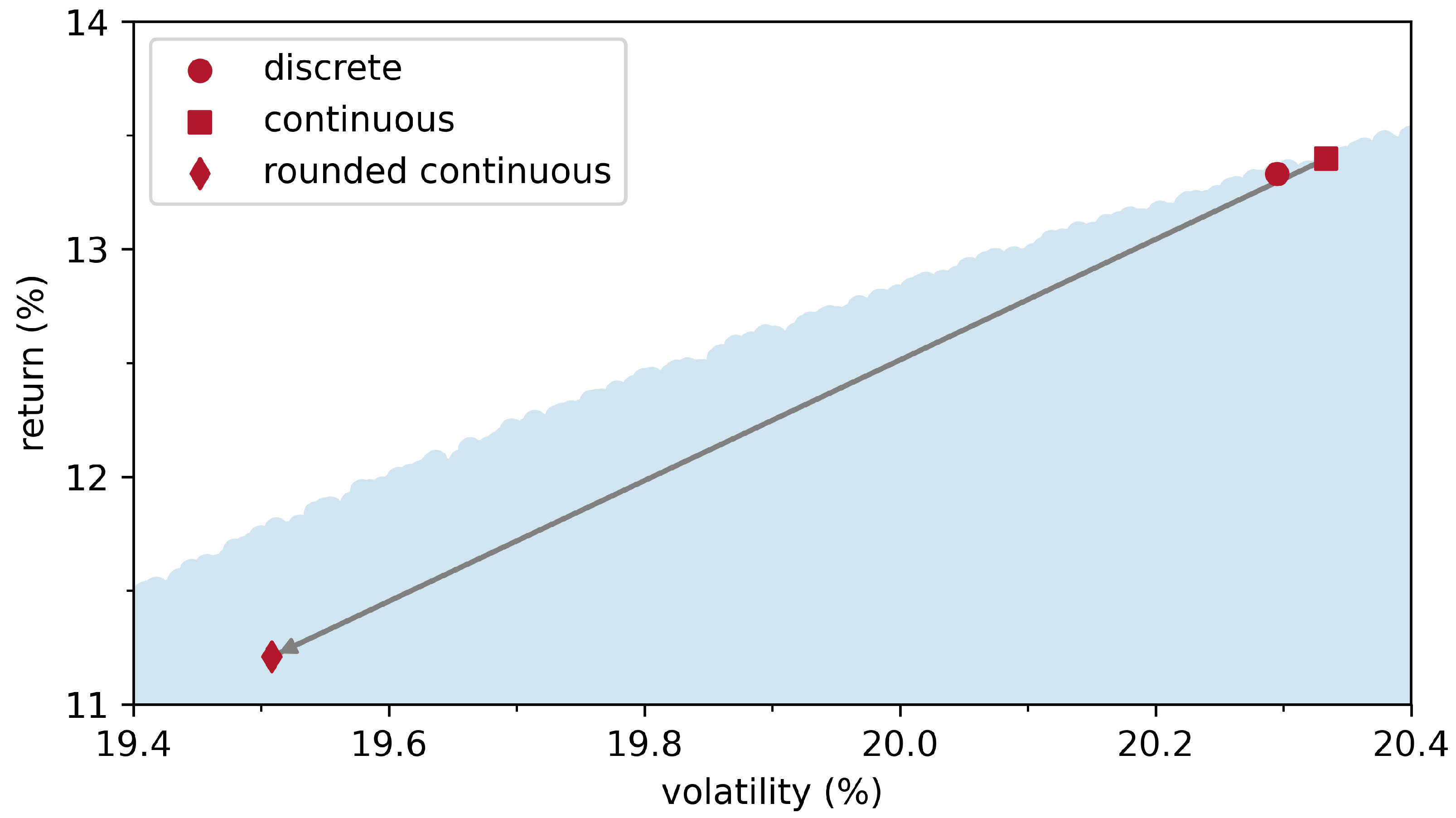
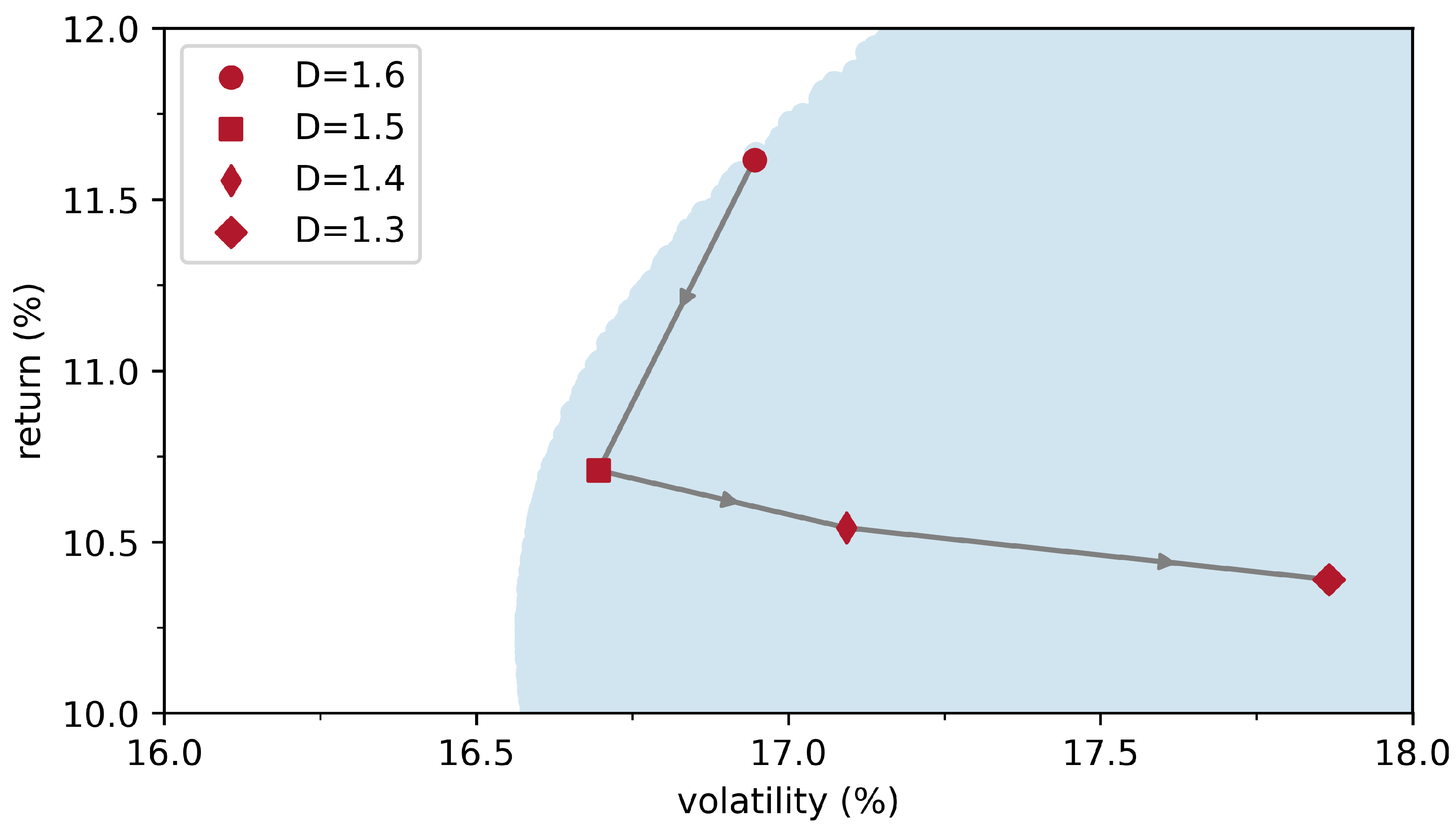
2.3. Incorporation of ESG Data into Markowitz Portfolio Theory

We have to address two questions in order to include ESG data into Markowitz portfolio optimization: (i) how to classify portfolios in terms of ESG scores and (ii) how to incorporate such information into the optimization scheme. The current literature on this topic can be divided into two main approaches: The most commonly found method of including ESG data is to constrain the Markowitz utility function so that it yields a portfolio with the weighted average of the expected ESG scores (Alessandrini and Jondeau 2021; Branda 2015; Cesarone et al. 2022; Chen et al. 2021; De Spiegeleer et al. 2023; Hirschberger et al. 2013; López Prol and Kim 2022; Maree and Omlin 2022; Shushi 2022; Utz et al. 2014; Varmaz et al. 2022), which actually constrains the possible portfolio compositions. The second approach (Lauria et al. 2022) employs an affine transformation between returns and ESG scores, which is controlled by an additional parameter.

Obviously, the composition-weighted average of expected ESG scores is not the only property that can be used to classify portfolios. In this subsection, we introduce a novel scheme for classifying portfolios in terms of the ESG score, which we incorporate into the discrete portfolio optimization scheme explained in Section 2.2.

We assume that the value of the ESG score S in every scoring system is bounded by the best and worst possible scores $S\in [S^{-},S^{+}]$. Let us consider a relative portfolio composition $\overrightarrow{\pi }$ with respect to the ESG scores of a given scoring system. Since the entries of $\overrightarrow{\pi }$ are non-negative and their sum is one, the entries of $\overrightarrow{\pi }$ can be interpreted as a probability distribution. As a reference point, we take a portfolio which only contains stocks with the best possible ESG score $S^{+}$. With the result of Wasserstein (Peyré and Cuturi 2019), the distances of other relative portfolio compositions with respect to this best possible portfolio can be calculated. Note that there may be multiple portfolio compositions in terms of stock allocation which possess the best possible score $S^{+}$, e.g., more than one stock in the investment universe has the best possible score. However, this possible degeneracy is irrelevant in our approach, as we will see.

If we use the Wasserstein metric in the case of two one-dimensional sets of measurements and take the limit of infinite number of observations (Kolouri et al. 2017; Villani 2003), we can write the Wasserstein p-distance between a given relative portfolio composition $\overrightarrow{\pi }$ and the best possible portfolio in the following way:

$$D_{\mathrm{ESG}}(p,\overrightarrow{\pi })={\left[\sum _i\left({\pi }_i·{\left|S^{+}-{\tilde{S}}_i\right|}^p\right)\right]}^{1/p}.$$

(15)

Here, i enumerates the possible values ${\tilde{S}}_i$ of the ESG score within the given portfolio $\overrightarrow{\pi }$. This vector contains the relative number of stock allocations to the respective ESG score ${\tilde{S}}_i$. ${\pi }_i$ is the i-th component of the vector $\overrightarrow{\pi }$. $p\in [1,+\infty )$ is the parameter of the Wasserstein p-distance. Note how the exact composition in terms of stocks is irrelevant in this approach. The distance measure $D_{\mathrm{ESG}}$ is only sensitive to the ESG scores of the respective constituents. Therefore, different allocations of stocks with the same ESG score do not affect $D_{\mathrm{ESG}}$. Also note that comparison to a best possible individual allocation would have required us to know this specific portfolio. This target portfolio is, however, in general unknown. The point of our method is to find it. Hence, we have chosen an approach in which knowledge of this hard-to-find solution is not required.

If all constituents of a portfolio $\overrightarrow{\pi }$ have the best possible score $S^{+}$, the distance measure is $D_{\mathrm{ESG}}(p,\overrightarrow{\pi })=0$. If all constituents of a portfolio $\overrightarrow{\pi }$ have the worst possible score $S^{-}$, the distance measure is $D_{\mathrm{ESG}}(p,\overrightarrow{\pi })=\left|S^{+}-S^{-}\right|$. Therefore, all other portfolios have $D_{\mathrm{ESG}}\left(p\right)\in \left[0,\left|S^{+}-S^{-}\right|\right]$ independently of p. In particular, if, for two given portfolios ${\overrightarrow{\pi }}_1$ and ${\overrightarrow{\pi }}_2$, we have $D_{\mathrm{ESG}}(p,{\overrightarrow{\pi }}_1)<D_{\mathrm{ESG}}(p,{\overrightarrow{\pi }}_2)$, then ${\overrightarrow{\pi }}_1$ has a better ESG score.

For $p=1$, our result in Equation (15) becomes the weighted average (up to a constant factor). Therefore, we may view Equation (15) as a generalized framework for classifying portfolios in terms of ESG scores. This framework does not depend on whether the best score $S^{+}$ has the lowest or the highest value in the respective scoring system. Also note that our distance measure may be generalized to work with heterogeneous data from different ESG data providers by using the relative distance of the single portfolio component within its pertinent ESG score range by extending Equation (15) with an additional normalization factor:

$$D_{\mathrm{ESG}}(p,\overrightarrow{\pi })={\left[\sum _i\left({\pi }_i·\frac{{\left|S^{+}\left({\pi }_i\right)-{\tilde{S}}_i\left({\pi }_i\right)\right|}^p}{{\left|S^{+}\left({\pi }_i\right)-S^{-}\left({\pi }_i\right)\right|}^p}\right)\right]}^{1/p}$$

(16)

Here, $S^{+}\left({\pi }_i\right),S^{-}\left(\pi \right),\widetilde{S_i}\left({\pi }_i\right)$ indicate, respectively, the best, the lowest and the spot score in the ESG system pertinent to the component ${\pi }_i$. Although our methodology would enable us to mix multiple ESG scoring systems, we do not expand upon this topic in the present manuscript and leave it for future research instead. In the present manuscript, we only use ESG data provided by ISS ESG.

To now, we have written the distance measure in terms of the relative composition with respect to the ESG score. In order to include the ESG data into the discrete optimization framework, we need to establish the ESG distance measure in terms of the composition with respect to the allocation of individual stocks. It is easy to show that Equation (15) can equivalently be written as:

$$D_{\mathrm{ESG}}(p,\overrightarrow{x})={\left[\sum _{i=1}^k\left(\frac{x_i}{N_{\mathrm{tot}}}·{\left|S^{+}-S_i\right|}^p\right)\right]}^{1/p}.$$

(17)

Here, $x_i$ is the i-th component of the discrete portfolio allocation vector $\overrightarrow{x}$ and $S_i$ is the ESG score of the i-th component stock in the portfolio. All other quantities are defined as before.

The Wasserstein p-distance is defined for $p\in [1,+\infty )$. Since the function $f\left(x\right)=x^p$ is strictly increasing for $p\ge 1$ and $x>0$, we know that $D_{\mathrm{ESG}}(p,\overrightarrow{x})$ from Equation (17) has a global maximum equal to $D_{max}=\left|S^{+}-S^{-}\right|$. Therefore, we can include a linear constraint on $D_{\mathrm{ESG}}(p,\overrightarrow{x})$ into the discrete optimization problem from Section 2.2 for every $p\ge 1$. The respective problem then reads:

$$min\left\{Q_d(\overrightarrow{r},\Sigma ,{\varphi }_c,N_{\mathrm{tot}})\right\}=min\left\{\frac{{\varphi }_c}{2N_{\mathrm{tot}}}{\overrightarrow{x}}^T\Sigma \overrightarrow{x}-{\overrightarrow{r}}^T\overrightarrow{x}\right\}.$$

(18)

The minimization of this utility function is subject to the following constraints:

$$\begin{array}{cc}\hfill & \overrightarrow{x}=(x_1,\cdots ,x_k)\mathrm{with}{x}_i\in \mathbb{N}\forall i,\hfill \\ \hfill & \sum _{i=1}^k{x}_i=N_{\mathrm{tot}},\hfill \\ \hfill & {\overrightarrow{p}}^T\overrightarrow{x}-B\le 0,\hfill \\ \hfill & D_{\mathrm{ESG}}(p,\overrightarrow{x})\le D.\hfill \end{array}$$

(19)

Note how the utility function in Equation (18) is unchanged compared to Equation (4) and Equation (12). The difference lies only in the additional constraint in Equation (19). Here, D is a non-negative constant. For $D\ge D_{max}$, this constraint has no effect on the optimal portfolio composition $\overrightarrow{x}$. For $D=0$, only stocks with the best possible score are allowed. In between these two extremes, the constraint restricts possible solutions to the given maximum distance in ESG rating space. In practice, we use $p=1$ and the latest ESG date in the period under investigation to calculate $D_{\mathrm{ESG}}(p=1,\overrightarrow{x})$. Exploring the effect of other choices for p is left for future studies.

We now perform calculations with the following stock universe reported in order from highest to lowest ESG score: Deutsche Telekom (ISIN DE0005557508), SAP (ISIN DE0007164600), Intesa Sanpaolo (ISIN IT0000072618) and EssilorLuxottica (ISIN FR0000121667). The portfolio optimization problem from Equations (18) and (19) was again solved on a D-Wave quantum annealer for different values of the ESG constraint D. The ESG data were provided by ISS ESG. The grading system is on a scale from 4 to 1, where a higher number indicates a better ESG performance. We use a budget of B = EUR 100,000 and a risk-aversion parameter of $\varphi =8$. The result in volatility–return space is shown in Figure 5. We first set $D=5$ and obtained a solution with $D_{\mathrm{ESG}}=1.6$. Hence, we conclude that the actual maximum reachable ESG distance within the given investment universe is $D_{\mathrm{ESG}}=1.6$. We gradually decreased D from there until the solution visibly departed from the efficient frontier. The latter was again calculated by sampling random portfolio compositions. At a certain point, stronger constraints on $D_{\mathrm{ESG}}(p,\overrightarrow{x})$ produce portfolios that move farther away from the efficient frontier. This finding is consistent with the study by Cesarone et al. (2022).

We also analyzed the portfolio composition for different values of D. The results are shown in Figure 6. We found that decreasing the distance D from the best possible portfolio in ESG terms gradually increases the weight of stocks with better ESG scores compared to stocks with worse ESG scores, both in terms of the relative composition and budget allocation. Stocks of Intesa Sanpaolo are not part of the optimal portfolios due to their relatively unfavorable returns (not driven by ESG scores). We had to vary $N_{\mathrm{tot}}$ somewhat as a function of D so that the full budget can be allocated. As can be seen from Figure 6, allocation to Deutsche Telekom increases with decreasing D. Since stocks of Deutsche Telekom have a much lower price per stock than SAP and EssilorLuxottica, a higher number of stocks has to be allocated, which requires a larger $N_{\mathrm{tot}}$. The resulting budget allocations are summarized in

Table 1. Number of stocks and allocated budget ${\overrightarrow{p}}^T\overrightarrow{x}$ as a function of the maximum ESG distance D.

D	${\mathit{N}}_{\mathbf{tot}}$	${\overrightarrow{\mathit{p}}}^{\mathit{T}}\overrightarrow{\mathit{x}}$ in EUR
1.6	960	99,999.56
1.5	1112	99,998.61
1.4	1202	99,994.84
1.3	1305	99,932.86

.

In this subsection, we have introduced a novel distance measure for portfolios within the space of ESG scores based on the Wasserstein metric. We use this distance measure to constrain the search for optimal portfolios in volatility–return space to a certain vicinity of the best possible portfolio in ESG space. We have demonstrated that our approach yields sensible and interesting results in combination with discrete portfolio optimization on a quantum annealer.

3. Discussion

The approach we have presented here is based on historical data of covariance and returns. A further constraint such as the one on the ESG classification may not improve the performance of any portfolio within this framework. However, there is an ongoing discussion in the literature on whether ESG-aware investors generate higher returns than comparable non-ESG benchmarks in the long term and can realize a better performance during a global crisis. The results of investigations into the historically measured performance of stocks with strong and weak ESG ratings vary depending on the markets, ESG data and time periods considered for analysis (Amon et al. 2021; Atz et al. 2023; Auer and Schuhmacher 2016; Bae et al. 2021; Breedt et al. 2018; Cesarone et al. 2022; Demers et al. 2021; García et al. 2022; La Torre et al. 2020; Nofsinger and Varma 2014).

Cesarone et al. (2022) investigate mean-variance-ESG optimal portfolios and show how portfolio mean returns systematically move away from the efficient frontier the more weight is placed on optimizing the ESG scores of the respective portfolio (compare Figure 5). These authors use a continuous Markowitz framework and obtain results consistent with ours. In addition, we show that optimal discrete portfolios can be obtained from modern quantum annealers under realistic circumstances.

Auer and Schuhmacher (2016) study the impact of socially responsible investments on the performance of investment funds. They compare the returns of investment funds with different ESG ratings to the return of their respective benchmark index. They find that portfolios of European stocks with high ESG ratings often underperform with respect to their benchmark, while no consistent over or underperformance was observed in the Asia-Pacific region and the United States. This approach differs from ours in that Auer and Schuhmacher use benchmark indices as their reference point, while we compared portfolios on the mean-variance efficient frontier. In this sense, an overperformance of ESG-aware portfolios is possible in Auer and Schuhmacher’s approach, since they compare benchmark indices, which may have sub-optimal returns in the first place. Due to the different methodology, these authors’ results are not directly comparable to ours. Nevertheless, our results and those of Cesarone et al. (2022) can help to rationalize these findings. Both studies find that the deviation in ESG-aware portfolios from mean-variance optimal portfolios depends on the emphasis, which is put on the ESG optimization goal. In particular, the novel ESG distance measure we introduced could help to clarify the results of Auer and Schuhmacher in future studies.

Amon et al. (2021) find that portfolios with good ESG ratings can be constructed at a small cost in terms of returns. This is consistent with our findings and those of Cesarone et al. (2022), which both show that many portfolios with close to optimal returns can at the same time have good ESG ratings. In future studies, our ESG distance measure could be used to quantify the deviation in these ESG-aware portfolios from the best possible portfolio in the respective rating system.

García et al. (2022) investigate ESG ratings within a multi-objective optimization framework, focusing on portfolios composed of component stocks from the Dow Jones Industrial Average (DJIA) index. These authors solve an NP-hard realistic portfolio problem similar to ours, but use a heuristic evolutionary algorithm where we employ a quantum annealer. They find that better ESG ratings generally imply lower returns. Nevertheless, many portfolios with good ESG ratings possess favorable risk–return profiles and may even outperform benchmark indices like the DJIA. These results are consistent with our present study.

Breedt et al. (2018) perform a factor analysis based on a proprietary mean-variance optimization method. They find that ESG is not an independent factor; i.e., ESG information is already captured by other investment factors. They conclude that including ESG information into the investment process neither lowers nor improves the investment returns. We found that it is possible to construct ESG-aware portfolios which are very close to the efficient frontier. Hence, our results can be considered consistent with those of Breedt and coauthors.

Nofsinger and Varma (2014) find that socially responsible investment portfolios overperform in times of market crisis and underperform in other periods. They performed regression using several factor models. This methodology is very different from ours and other mean-variance approaches. Furthermore, the ESG selection is based on a screening approach, not on optimization. Again, over- and underperformance were measured with respect to regional benchmarks. Therefore, these results are not directly comparable to ours.

Demers et al. (2021) conduct a similar study and conclude that ESG-aware investment does not protect against market crises. Their argument is similar to that of Breedt et al. (2018), since they also conclude that ESG is not an independent investment factor.

Bae et al. (2021) perform a regression analysis and conclude that corporate social responsibility dis not affect the returns of US stocks during the COVID-19 market crisis. These authors also point out the possibility of firms having positive ESG values in certain rating systems, while actually acting against these goals in practice. Like other factor regression studies, these results are not directly comparable to ours.

La Torre et al. (2020) find that ESG ratings weakly affect the returns of EURO STOXX 50 component stocks. Their analysis is based on regression of a factor model, which is only loosely related to our study. Again, our quantitative distance measure in ESG space could help to clarify these results in future studies.

Atz et al. (2023) perform a meta-study on the impact of sustainability on investment returns. They argue that most studies find no discernible impact, while about one-third of all investigated studies find a positive impact. The positive impact is attributed to the possibility of capturing climate risk premiums and higher robustness during times of crisis.

As explained before, the question of whether ESG-aware investments produce measurable effects on investment performance is beyond the scope of this work. Such effects would result from investment decisions guided by beliefs and values, which are not captured by the Markowitz framework used in our study.

In our opinion, the question is ultimately to which degree investor expectations about future developments are reflected in historical prices. As we explained in the introduction, the importance of informed investment decisions based on ESG data can be expected to grow. The degree to which non-ESG-aware investors are following these developments is, however, unclear. Therefore, stocks with good ESG scores may outperform stocks with worse ESG scores, as the public increasingly demands the publication of ESG data and enforces the adoption of ESG-aware investment strategies. This effect is not captured by Markowitz portfolio theory and would require a radically different approach.

We expect that interest in ESG topics will grow rapidly among investors, particularly regarding portfolio classification in terms of ESG scores. Our method of using ESG data enables ESG-aware investors to construct ESG-friendly portfolios without the need for further assumptions or additional parameters. In particular, we avoid assuming additivity of ESG data with other terms in the Markowitz utility function. In fact, we do not modify the utility function at all, so that ESG data only appear in the linear constraint we introduced. Thus, in our approach, ESG preference, returns and volatility can be interpreted independently, as one would expect (Pedersen et al. 2021; Utz et al. 2014; Varmaz et al. 2022).

Our study also shows that portfolio optimization is an attractive case for combining classical and quantum workflows. While the discrete portfolio optimization problem can only be solved efficiently on a quantum computer, all data processing is still performed efficiently on a classical computer. We believe that many quantum applications will be part of such hybrid quantum–classical workflows in the future. See refs. (Cohen et al. 2020a, 2020b; Lang et al. 2022; Mugel et al. 2021; Sakuler et al. 2023; Venturelli and Kondratyev 2019) for more examples of hybrid approaches to portfolio optimization.

4. Conclusions

We have presented a study of Markowitz portfolio optimization in the presence of discrete stock allocations, a limited budget and constraints on portfolio ESG scores. We have studied both the usual continuous formulation of the portfolio problem as well as a more realistic discrete version. The discrete version cannot be solved efficiently on classical computers, at least not by enumerating all possible portfolio combinations, although some progress has been achieved using simulated annealing on classical hardware (Rubio-García et al. 2022). Therefore, we have employed a D-Wave quantum annealer for solving the discrete portfolio problem.

We have established a mapping between continuous and discrete Markowitz portfolio theories, which allows us to compare results in a meaningful way. This mapping involves a rescaling of the risk-aversion parameter $\varphi$. Importantly, we have also shown that when failing to apply this rescaling in the discrete case, the relative composition of discrete solutions will not converge to the continuous solution, even in the limit of an infinite portfolio size, but rather converge to the minimum variance portfolio.

Subsequently, we extended Markowitz portfolio theory to include a budget constraint. We showed that the rounding of continuous portfolio compositions to the nearest integer number of stocks yields sub-optimal portfolios for small and medium investment budgets. Solutions from our discrete approach on the contrary lie on the efficient frontier in volatility–return space.

Furthermore, we introduced a novel way to classify portfolios in terms of their ESG score via the Wasserstein p-distance by viewing relative portfolio compositions as discrete probability distributions. Using the Wasserstein metric, we measured a portfolio’s distance from the best possible portfolio using the ESG score in the respective scoring system. Our method is a generalization of the weighted average classification scheme reported in the literature and is applicable to any ESG scoring system without further modification. Our framework can even be modified to accommodate ESG data from heterogeneous scoring systems. We incorporated the ESG data into the optimization process by constraining the portfolio search to a certain maximum distance from the portfolio with the best possible ESG score via a linear constraint which is independent of the chosen metric.

We also reported case studies for portfolios using components of the well-known EURO STOXX 50 index. By decreasing the maximum distance from the best ESG portfolio, we found that portfolio compositions gradually placed more weight on stocks with better ESG scores and less weight on stocks with worse ESG scores, both in terms of the number of stocks and in terms of the allocated budget.

Our results can help ESG-aware investors include their preferences in an effective way, building on the widely used Markowitz portfolio theory. How these preferences are derived is a research field in itself and goes beyond our work.

We have only studied the Wasserstein p-distance for $p=1$. Future studies should clarify the role of p for the ESG portfolio problem. Furthermore, our method could be applied to larger portfolios and heterogeneous ESG data from different providers. We believe that the formalism we have presented can be applied to many practical problems, such as finding tradeable ESG-optimized portfolios or constructing discrete ESG-aware portfolios as a basis for exactly hedgeable indices. These topics are left for future research.

References

1. Abrams, Daniel S., and Seth Lloyd. 1998. Nonlinear quantum mechanics implies polynomial-time solution for np-complete and #p problems. Physical Review Letters 81: 3992–95. [Google Scholar] [CrossRef]
2. Agrawal, Akshay, Robin Verschueren, Steven Diamond, and Stephen Boyd. 2018. A rewriting system for convex optimization problems. Journal of Control and Decision 5: 42–60. [Google Scholar] [CrossRef]
3. Alessandrini, Fabio, and Eric Jondeau. 2021. Optimal strategies for esg portfolios. The Journal of Portfolio Management 47: 114–38. [Google Scholar] [CrossRef]
4. Amon, Julian, Margarethe Rammerstorfer, and Karl Weinmayer. 2021. Passive esg portfolio management—The benchmark strategy for socially responsible investors. Sustainability 13: 9388. [Google Scholar] [CrossRef]
5. Atz, Ulrich, Tracy Van Holt, Zongyuan Zoe Liu, and Christopher C. Bruno. 2023. Does sustainability generate better financial performance? review, meta-analysis, and propositions. Journal of Sustainable Finance & Investment 13: 802–25. [Google Scholar] [CrossRef]
6. Auer, Benjamin R., and Frank Schuhmacher. 2016. Do socially (ir)responsible investments pay? new evidence from international esg data. The Quarterly Review of Economics and Finance 59: 51–62. [Google Scholar] [CrossRef]
7. Bae, Kee-Hong, Sadok El Ghoul, Zhaoran Jason Gong, and Omrane Guedhami. 2021. Does csr matter in times of crisis? evidence from the COVID-19 pandemic. Journal of Corporate Finance 67: 101876. [Google Scholar] [CrossRef]
8. Berg, Florian, Julian F. Kölbel, and Roberto Rigobon. 2022. Aggregate Confusion: The Divergence of ESG Ratings. Review of Finance 26: 1315–44. [Google Scholar] [CrossRef]
9. Bonami, Pierre, and Miguel A. Lejeune. 2009. An exact solution approach for portfolio optimization problems under stochastic and integer constraints. Operations Research 57: 650–70. [Google Scholar] [CrossRef]
10. Branda, Martin. 2015. Diversification-consistent data envelopment analysis based on directional-distance measures. Omega 52: 65–76. [Google Scholar] [CrossRef]
11. Brandhofer, Sebastian, Daniel Braun, Vanessa Dehn, Gerhard Hellstern, Matthias Hüls, Yanjun Ji, Ilia Polian, Amandeep Singh Bhatia, and Thomas Wellens. 2022. Benchmarking the performance of portfolio optimization with qaoa. Quantum Information Processing 22: 25. [Google Scholar] [CrossRef]
12. Breedt, André, Stefano Ciliberti, Stanislao Gualdi, and Philip Seager. 2018. Is ESG an Equity Factor or Just an Investment Guide? Available online: https://ssrn.com/abstract=3207372 (accessed on 21 March 2024). [CrossRef]
13. Bruno, Michelangelo, and Valentina Lagasio. 2021. An overview of the european policies on esg in the banking sector. Sustainability 13: 12641. [Google Scholar] [CrossRef]
14. Buonaiuto, Giuseppe, Francesco Gargiulo, Giuseppe De Pietro, Massimo Esposito, and Marco Pota. 2023. Best practices for portfolio optimization by quantum computing, experimented on real quantum devices. Scientific Reports 13: 19434. [Google Scholar] [CrossRef] [PubMed]
15. Castro, Francisco, Jesús Gago, Isabel Hartillo, Justo Puerto, and Jose Maria Ucha. 2011. An algebraic approach to integer portfolio problems. European Journal of Operational Research 210: 647–59. [Google Scholar] [CrossRef]
16. Cesarone, Francesco, Manuel Luis Martino, and Alessandra Carleo. 2022. Does esg impact really enhance portfolio profitability? Sustainability 14: 2050. [Google Scholar] [CrossRef]
17. Chen, Bingren, Hanqing Wu, Haomu Yuan, Lei Wu, and Xin Li. 2023. Quantum portfolio optimization: Binary encoding of discrete variables for qaoa with hard constraint. arXiv arXiv:2304.06915. [Google Scholar] [CrossRef]
18. Chen, Li, Lipei Zhang, Jun Huang, Helu Xiao, and Zhongbao Zhou. 2021. Social responsibility portfolio optimization incorporating esg criteria. Journal of Management Science and Engineering 6: 75–85. [Google Scholar] [CrossRef]
19. Cohen, Jeffrey, Alex Khan, and Clark Alexander. 2020a. Portfolio optimization of 40 stocks using the dwave quantum annealer. arXiv arXiv:2007.01430. [Google Scholar] [CrossRef]
20. Cohen, Jeffrey, Alex Khan, and Clark Alexander. 2020b. Portfolio optimization of 60 stocks using classical and quantum algorithms. arXiv arXiv:2008.08669. [Google Scholar] [CrossRef]
21. Coleman, Thomas F., Yuying Li, and Jay Henniger. 2006. Minimizing tracking error while restricting the number of assets. Journal of Risk 8: 33. [Google Scholar] [CrossRef]
22. Demers, Elizabeth, Jurian Hendrikse, Philip Joos, and Baruch Lev. 2021. Esg did not immunize stocks during the COVID-19 crisis, but investments in intangible assets did. Journal of Business Finance & Accounting 48: 433–62. [Google Scholar] [CrossRef]
23. De Spiegeleer, Jan, Stephan Höcht, Daniel Jakubowski, Sofie Reyners, and Wim Schoutens. 2023. Esg: A new dimension in portfolio allocation. Journal of Sustainable Finance & Investment 13: 827–67. [Google Scholar] [CrossRef]
24. Diamond, Steven, and Stephen Boyd. 2016. CVXPY: A Python-embedded modeling language for convex optimization. Journal of Machine Learning Research 17: 1–5. [Google Scholar]
25. D-Wave Systems Inc. 2021. Hybrid Solver for Constrained Quadratic Models. Technical Report 14-1055A-A. Burnaby: D-Wave Systems Inc. [Google Scholar]
26. Elsokkary, Nada, Faisal Shah Khan, Davide La Torre, Travis S. Humble, and Joel Gottlieb. 2017. Financial Portfolio Management Using d-Wave Quantum Optimizer: The Case of Abu Dhabi Securities Exchange. Technical Report. Oak Ridge: Oak Ridge National Lab. (ORNL). [Google Scholar]
27. Farhi, Edward, Jeffrey Goldstone, and Sam Gutmann. 2014. A quantum approximate optimization algorithm. arXiv arXiv:1411.4028. [Google Scholar] [CrossRef]
28. García, Fernando, Tsvetelina Gankova-Ivanova, Jairo González-Bueno, Javier Oliver, and Rima Tamošiūnienė. 2022. What is the cost of maximizing ESG performance in the portfolio selection strategy? The case of The Dow Jones Index average stocks. Entrepreneurship and Sustainability Issues 9: 178–92. [Google Scholar] [CrossRef] [PubMed]
29. Grant, Erica, Travis S. Humble, and Benjamin Stump. 2021. Benchmarking quantum annealing controls with portfolio optimization. Physical Review Applied 15: 014012. [Google Scholar] [CrossRef]
30. Herman, Dylan, Cody Googin, Xiaoyuan Liu, Yue Sun, Alexey Galda, Ilya Safro, Marco Pistoia, and Yuri Alexeev. 2023. Quantum computing for finance. Nature Reviews Physics 5: 450–65. [Google Scholar] [CrossRef]
31. Hirschberger, Markus, Ralph E. Steuer, Sebastian Utz, Maximilian Wimmer, and Yue Qi. 2013. Computing the nondominated surface in tri-criterion portfolio selection. Operations Research 61: 169–83. [Google Scholar] [CrossRef]
32. Jacquier, Antoine, Oleksiy Kondratyev, Alexander Lipton, and Marcos Lopez de Prado. 2022. Quantum Machine Learning and Optimisation in Finance: On the Road to Quantum Advantage. Birmingham: Packt Publishing. [Google Scholar]
33. Jobst, Norbert J., Michael D. Horniman, Cormac A. Lucas, and Gautam Mitra. 2001. Computational aspects of alternative portfolio selection models in the presence of discrete asset choice constraints. Quantitative Finance 1: 489. [Google Scholar] [CrossRef]
34. Kellerer, Hans, Renata Mansini, and M. Grazia Speranza. 2000. Selecting portfolios with fixed costs and minimum transaction lots. Annals of Operations Research 99: 287–304. [Google Scholar] [CrossRef]
35. King, Andrew D., Jack Raymond, Trevor Lanting, Richard Harris, Alex Zucca, Fabio Altomare, Andrew J. Berkley, Kelly Boothby, Sara Ejtemaee, Colin Enderud, and et al. 2023. Quantum critical dynamics in a 5000-qubit programmable spin glass. Nature 617: 61–66. [Google Scholar] [CrossRef] [PubMed]
36. Kolm, Petter N., Reha Tütüncü, and Frank J. Fabozzi. 2014. 60 years of portfolio optimization: Practical challenges and current trends. European Journal of Operational Research 234: 356–71. [Google Scholar] [CrossRef]
37. Kolouri, Soheil, Se Rim Park, Matthew Thorpe, Dejan Slepcev, and Gustavo K. Rohde. 2017. Optimal mass transport: Signal processing and machine-learning applications. IEEE Signal Processing Magazine 34: 43–59. [Google Scholar] [CrossRef] [PubMed]
38. Lang, Jonas, Sebastian Zielinski, and Sebastian Feld. 2022. Strategic portfolio optimization using simulated, digital, and quantum annealing. Applied Sciences 12: 12288. [Google Scholar] [CrossRef]
39. Larcker, David F., Lukasz Pomorski, Brian Tayan, and Edward Watts. 2022. Esg Ratings: A Compass without Direction. Rock Center for Corporate Governance at Stanford University Working Paper Forthcoming. Available online: https://ssrn.com/abstract=4179647 (accessed on 21 March 2024).
40. La Torre, Mario, Fabiomassimo Mango, Arturo Cafaro, and Sabrina Leo. 2020. Does the esg index affect stock return? evidence from the eurostoxx50. Sustainability 12: 6387. [Google Scholar] [CrossRef]
41. Lauria, Davide, W. Brent Lindquist, Stefan Mittnik, and Svetlozar T. Rachev. 2022. Esg-valued portfolio optimization and dynamic asset pricing. arXiv arXiv:2206.02854. [Google Scholar] [CrossRef]
42. Li, Han-Lin, and Jung-Fa Tsai. 2008. A distributed computation algorithm for solving portfolio problems with integer variables. European Journal of Operational Research 186: 882–91. [Google Scholar] [CrossRef]
43. López Prol, Javier, and Kiwoong Kim. 2022. Risk-return performance of optimized esg equity portfolios in the nyse. Finance Research Letters 50: 103312. [Google Scholar] [CrossRef]
44. Lucas, Andrew. 2014. Ising formulations of many np problems. Frontiers in Physics 2: 5. [Google Scholar] [CrossRef]
45. Mansini, Renata, and Maria Grazia Speranza. 1999. Heuristic algorithms for the portfolio selection problem with minimum transaction lots. European Journal of Operational Research 114: 219–33. [Google Scholar] [CrossRef]
46. Maree, Chari, and Christian W. Omlin. 2022. Balancing profit, risk, and sustainability for portfolio management. Presented at 2022 IEEE Symposium on Computational Intelligence for Financial Engineering and Economics (CIFEr), Helsinki, Finland, May 4–5; New York: IEEE, pp. 1–8. [Google Scholar] [CrossRef]
47. Markowitz, Harry. 1952. Portfolio selection. The Journal of Finance 7: 77–91. [Google Scholar] [CrossRef]
48. Mugel, Samuel, Carlos Kuchkovsky, Escolástico Sánchez, Samuel Fernández-Lorenzo, Jorge Luis-Hita, Enrique Lizaso, and Román Orús. 2022. Dynamic portfolio optimization with real datasets using quantum processors and quantum-inspired tensor networks. Physical Review Research 4: 013006. [Google Scholar] [CrossRef]
49. Mugel, Samuel, Mario Abad, Miguel Bermejo, Javier Sánchez, Enrique Lizaso, and Román Orús. 2021. Hybrid quantum investment optimization with minimal holding period. Scientific Reports 11: 19587. [Google Scholar] [CrossRef] [PubMed]
50. Nofsinger, John, and Abhishek Varma. 2014. Socially responsible funds and market crises. Journal of Banking & Finance 48: 180–93. [Google Scholar] [CrossRef]
51. Orús, Román, Samuel Mugel, and Enrique Lizaso. 2019. Quantum computing for finance: Overview and prospects. Reviews in Physics 4: 100028. [Google Scholar] [CrossRef]
52. Palmer, Samuel, Konstantinos Karagiannis, Adam Florence, Asier Rodriguez, Roman Orus, Harish Naik, and Samuel Mugel. 2022. Financial index tracking via quantum computing with cardinality constraints. arXiv arXiv:2208.11380. [Google Scholar] [CrossRef]
53. Pedersen, Lasse Heje, Shaun Fitzgibbons, and Lukasz Pomorski. 2021. Responsible investing: The esg-efficient frontier. Journal of Financial Economics 142: 572–97. [Google Scholar] [CrossRef]
54. Peyré, Gabriel, and Marco Cuturi. 2019. Computational optimal transport: With applications to data science. Foundations and Trends® in Machine Learning 11: 355–607. [Google Scholar] [CrossRef]
55. Phillipson, Frank, and Harshil Singh Bhatia. 2021. Portfolio optimisation using the d-wave quantum annealer. In International Conference on Computational Science. New York: Springer, pp. 45–59. [Google Scholar] [CrossRef]
56. Romero, Sebastián V., Eneko Osaba, Esther Villar-Rodriguez, Izaskun Oregi, and Yue Ban. 2023. Hybrid approach for solving real-world bin packing problem instances using quantum annealers. Scientific Reports 13: 11777. [Google Scholar] [CrossRef] [PubMed]
57. Rosenberg, Gili, Poya Haghnegahdar, Phil Goddard, Peter Carr, Kesheng Wu, and Marcos López de Prado. 2016. Solving the optimal trading trajectory problem using a quantum annealer. IEEE Journal of Selected Topics in Signal Processing 10: 1053–60. [Google Scholar] [CrossRef]
58. Rubio-García, Álvaro, Juan José García-Ripoll, and Diego Porras. 2022. Portfolio optimization with discrete simulated annealing. arXiv arXiv:2210.00807. [Google Scholar] [CrossRef]
59. Sakuler, Wolfgang, Johannes M. Oberreuter, Riccardo Aiolfi, Luca Asproni, Branislav Roman, and Jürgen Schiefer. 2023. A real world test of portfolio optimization with quantum annealing. arXiv arXiv:2303.12601. [Google Scholar] [CrossRef]
60. Shunza, Justus, Mary Akinyemi, and Chika Yinka-Banjo. 2023. Application of quantum computing in discrete portfolio optimization. Journal of Management Science and Engineering 8: 453–64. [Google Scholar] [CrossRef]
61. Shushi, Tomer. 2022. The optimal solution of esg portfolio selection models that are based on the average esg score. Operations Research Letters 50: 513–16. [Google Scholar] [CrossRef]
62. Streichert, Felix, Holger Ulmer, and Andreas Zell. 2004. Evolutionary algorithms and the cardinality constrained portfolio optimization problem. In Operations Research Proceedings 2003: Selected Papers of the International Conference on Operations Research (OR 2003), Heidelberg, Germany, September 3–5. New York: Springer, pp. 253–60. [Google Scholar] [CrossRef]
63. Utz, Sebastian, Maximilian Wimmer, Markus Hirschberger, and Ralph E. Steuer. 2014. Tri-criterion inverse portfolio optimization with application to socially responsible mutual funds. European Journal of Operational Research 234: 491–98. [Google Scholar] [CrossRef]
64. Varmaz, Armin, Christian Fieberg, and Thorsten Poddig. 2022. Portfolio Optimization for Sustainable Investments. Available online: https://ssrn.com/abstract=3859616 (accessed on 21 March 2024).
65. Venturelli, Davide, and Alexei Kondratyev. 2019. Reverse quantum annealing approach to portfolio optimization problems. Quantum Machine Intelligence 1: 17–30. [Google Scholar] [CrossRef]
66. Vielma, Juan Pablo, Shabbir Ahmed, and George L. Nemhauser. 2008. A lifted linear programming branch-and-bound algorithm for mixed-integer conic quadratic programs. INFORMS Journal on Computing 20: 438–50. [Google Scholar] [CrossRef]
67. Villani, Cedric. 2003. Topics in Optimal Transportation. Graduate Studies in Mathematics. Providence: American Mathematical Society. [Google Scholar]
68. Young, Martin R. 1998. A minimax portfolio selection rule with linear programming solution. Management Science 44: 673–83. [Google Scholar] [CrossRef]
69. Zheng, Chao. 2021. Universal quantum simulation of single-qubit nonunitary operators using duality quantum algorithm. Scientific Reports 11: 3960. [Google Scholar] [CrossRef] [PubMed]
Figure 1. Euclidean norm of the difference vector between optimal relative portfolio weights x for the continuous ( x c ) and discrete optimization case ( x d ). The risk-aversion parameter is set to ϕ = 8 , but different choices of ϕ > 0 give similar results. The investment universe comprises BMW (ISIN DE0005190003), Deutsche Post (ISIN DE0005552004), Deutsche Telekom (ISIN DE0005557508) and Infineon (ISIN DE0006231004). Data were taken from the period between 1 January 2010 and 1 January 2021. Lines are guides for the eye. (a) Difference between continuous solution and naive discrete approach (circles), as well as the difference between continuous and normalized discrete solutions (squares). Obviously, the naive approach does not converge to the continuous solution, even for very large portfolios. The normalized discrete approach converges to the well-known continuous solution for large portfolios. The remaining differences in portfolio composition are purely due to the discreteness. (b) Difference between continuous and naive discrete solutions for the modified utility function Q mod = x T Σ x , which only includes the covariance term. It is clearly visible that both the continuous and discrete approaches converge to the same minimum variance portfolio for this modified utility function Q mod . Also here, the remaining differences in portfolio composition are purely due to the discreteness.
Risks 12 00066 g001
Figure 2. Portfolio positions in volatility–return space for the naive discrete optimization approach as a function of the total number of stocks N tot in the portfolio. The risk-aversion parameter is set to ϕ = 1 . The investment universe comprises BMW (ISIN DE0005190003), Deutsche Post (ISIN DE0005552004), Deutsche Telekom (ISIN DE0005557508) and Infineon (ISIN DE0006231004). The light blue background is generated by randomly sampling the space of possible portfolios. The upper boundary of the light blue area is commonly called the ‘efficient frontier’. Data were taken from the period between 1 January 2010 and 1 January 2021. Lines and arrows are guides for the eye.
Risks 12 00066 g002
Figure 3. Best portfolio compositions for a budget of B = EUR 100,000 and risk-aversion parameter of ϕ = 8 . The discrete solution is obtained by minimizing the utility function in Equation (12) under the constraints of Equation (13). We use N tot = 3401 . The continuous results were obtained by multiplying the relative allocation by the available budget and rounding to integer stocks via Equation (14), which resulted in N tot = 4026 . The investment universe comprises BMW (ISIN DE0005190003), Deutsche Post (ISIN DE0005552004), Deutsche Telekom (ISIN DE0005557508) and Infineon (ISIN DE0006231004). Data were taken from the period between 1 January 2010 and 1 January 2021. (a) Portfolio composition in terms of number of stocks. (b) Portfolio composition in terms of Euro value.
Risks 12 00066 g003
Figure 4. Position of the best portfolio compositions in volatility–return space for a budget of B = EUR 100,000 and a risk-aversion parameter of ϕ = 8 . The discrete solution is obtained by minimizing the utility function in Equation (12) under the constraints of Equation (13). We use N tot = 3401 . The continuous results were obtained by multiplying the relative allocation by the available budget and rounding to integer stocks via Equation (14), which results in N tot = 4026 . The investment universe comprises BMW (ISIN DE0005190003), Deutsche Post (ISIN DE0005552004), Deutsche Telekom (ISIN DE0005557508) and Infineon (ISIN DE0006231004). Data were taken from the period between 1 January 2010 and 1 January 2021. The discrete solution is clearly at the efficient frontier, while the rounded continuous solution is visibly sub-optimal. Arrows are guides for the eye.
Risks 12 00066 g004
Figure 5. Position of the best discrete portfolio compositions in volatility–return space for a budget of B = EUR 100,000, a risk-aversion parameter of ϕ = 8 and different values of the maximum allowed ESG distance D. The ESG data were provided by ISS ESG. The grading system is on a scale from 4 to 1, where a higher number indicates a better ESG performance. The investment universe comprises Deutsche Telekom (ISIN DE0005557508), SAP (ISIN DE0007164600), Intesa Sanpaolo (ISIN IT0000072618) and EssilorLuxottica (ISIN FR0000121667), which are given in order from highest to lowest ESG score. Data were taken from the period between 1 January 2010 and 1 January 2021. The solution portfolios move away from the efficient frontier as we restrict them into a space that becomes gradually tighter around the best possible ESG score. Arrows are guides for the eye.
Risks 12 00066 g005
Figure 6. Best discrete portfolio compositions for a budget of B = EUR 100,000, a risk-aversion parameter of ϕ = 8 and different values of the maximum allowed ESG distance D. The ESG data were provided by ISS ESG. The grading system is on a scale from 4 to 1, where a higher number indicates a better ESG performance. The investment universe comprises Deutsche Telekom (ISIN DE0005557508), SAP (ISIN DE0007164600), Intesa Sanpaolo (ISIN IT0000072618) and EssilorLuxottica (ISIN FR0000121667), which are given in order from highest to lowest ESG score. Data were taken from the period between 1 January 2010 and 1 January 2021. Decreasing the maximum distance D to the portfolio with best possible ESG score results in compositions which gradually contain higher amounts of stocks with better ESG scores such as Deutsche Telekom and SAP. (a) Portfolio composition in terms of number of stocks. (b) Portfolio composition in terms of Euro value.
Risks 12 00066 g006