The Exponential Dispersion Family (EDF) Chain Ladder and Data Granularity

Abstract

This paper is concerned with the choice of data granularity for application of the EDF (Exponential Dispersion Family) chain ladder model to forecast a loss reserve. As the duration of individual accident and development periods is decreased, the number of data points increases, but the volatility of each point increases. This leads to a question as to whether a decrease in time unit leads to an increase or decrease in the variance of the loss reserve estimate. Is there an optimal granularity with respect to the variance of the loss reserve? A preliminary question is that of whether an EDF chain ladder that is valid for one duration (here called mesh size) remains so for another. The conditions under which this is so are established. There are various ways in which the mesh size of a data triangle may be varied. The paper identifies two of particular interest. For each of these two types of variation, the effect on variance of loss reserve is studied. Subject to some technical qualifications, the conclusion is that an increase in mesh size always increases the variance. It follows that one should choose a very high degree of granularity in order to maximize efficiency of loss reserve forecasting.

1. Introduction

1.1. Background

The chain ladder is a widely used model for insurance loss reserving (Mack 1993; Taylor 1985, 2000; Wüthrich and Merz 2008). The data set to which it is applied is typically triangular, with rows labelled by accident period and columns by development period.

Accident and development periods are commonly years, but other units of time are possible, e.g., quarters, months, weeks, etc. As the time unit is decreased, the number of data points increases, but the variance of each point increases. This leads to a question as to whether a decrease in time unit leads to an increase or decrease in the variance of the loss reserve estimate. A typical question faced by a practitioner might be the following one.

Example 1. 

Past chain ladder analyses of data triangles have been performed on quarterly data. The next valuation of liability could be conducted in the same way. However, monthly data are also available, and so application of the chain ladder to a monthly data triangle is also feasible. Is this likely to lead to a more or less reliable (as measured by predictive variance) estimate of liability?

A natural companion to this question is whether there is an optimal time unit at which the variance of the forecast loss reserve is minimized.

This question arises in numerous scientific contexts, e.g., statistics, energy, demand forecasting, finance, medicine, traffic flow and air quality, to name some.

Cases that closely mirror the question investigated in this paper include Kim et al. (2022), Z. Wang et al. (2023), Das et al. (2022), Grolinger et al. (2016), Li et al. (2019) and Jain et al. (2014). All of these point out that the calibration of statistical models can depend on the choice of data granularity, and propose methods for making this choice.

Other papers are not specifically concerned with optimization of granularity, but still point out that it can affect accuracy and efficiency of modelling. Examples are Elton et al. (2010), Huang and Zhu (2016), Lusis et al. (2017) and J. Wang et al. (2020).

While some of the actuarial literature discusses the choice of granularity of data for claim modelling in general terms, it remains silent on the specific questions just stated.

Even practitioner textbooks offer little. For example, an American text (Peterson 1981, p. 122) makes the following statement:

“Annual exposure periods [accident periods] and development intervals are used in this example, but shorter periods can also be used; quarterly semi-annual or monthly periods are the most common, other than annual.”

Similarly, an Australian text (Hart et al. 1996, p. 226) includes the statement:

“The difference between the payment year and the accident year is referred to as the development year. Other time periods can also be used particularly for short-tail classes.”

Both of these volumes refer to the possibility of different data granularities, but with no advice on the selection of a specific one. Associated general comment implies that the length of development periods might be chosen to be broadly proportional to the average delay from occurrence to closure of claims, but no reasoning for this is given.

1.2. Purpose of the Paper

The present paper aims to address those questions. It is necessary that a discussion of the chain ladder recognize two quite distinct formulations of that model. These are:

• The EDF chain ladder (Wüthrich and Merz 2008; Taylor 2009), where EDF refers to the exponential dispersion family; and
• The Mack chain ladder (Mack 1993).

These two models differ in a number of ways, but the main difference relevant to the present discussion is that, in the former, a distribution (EDF, in fact) is placed on each data point, whereas in the latter observations are distribution-free (though subject to an assumed variance).

The questions raised in Section 1.1 can be addressed for each type of model, but the difference just identified necessitates different mathematical approaches. As the title of the present paper indicates, it deals with the EDF chain ladder model, and especially the sub-models Tweedie chain ladder and Poisson chain ladder. A sequel paper deals with the Mack chain ladder.

The present paper thus discusses the influence of data granularity on the variance of the loss reserve forecast by the EDF chain ladder. Under suitable conditions, it is possible to identify the granularity that minimizes this variance.

1.3. Layout of the Paper

The paper considers changes of mesh size on the triangular data set, which is to say changes in the units of time used for accident and development periods. The effect of an increase in mesh size (i.e., an increase in the length of time spanned by one of these periods) on the variance of the estimated loss reserve is investigated.

There are various ways in which the mesh size of a data set can be varied. Some are more sensible than others, and two fundamental types of variation are considered here. Both, though subject to limitation, are extremely versatile. One is of a type usually found in practice; the other, though not unknown in practice, is rarer, but possessed of one or two useful properties. These types of variation are described in Section 2.

Since, under the EDF chain ladder, observations come equipped with distributions, sufficient statistics can be sought and put to use. These types of statistics are also discussed in Section 2.

Section 3 largely recites the background literature, introducing the EDF, Tweedie and Poisson chain ladders, their parameter estimation algorithms, and discusses the sufficient statistics associated with each. Section 4 and Section 5 then contain this paper’s own further development, examining the effect of changed mesh size on the variance of estimated loss reserve. These two sections deal with the two types of mesh variation just described, and how they influence the variance of the EDF chain ladder loss reserve. A numerical example of the findings of Section 5 is given in Section 6. Finally, Section 7 summarizes and discusses the findings of these sections.

2. Notation and Mathematical Preliminaries

2.1. Fundamentals

Let $i=1,2,\dots ,I$ denote accident period and $j=0,1,\dots ,I-1$ development period. Let $Y_{ij}$, with mean ${\mu }_{ij}$, denote the random variable representing the amount of claim payments made during development period $j$ of accident period $i$. These are usually referred to as incremental claim payments. All accident and development periods are of equal duration, though this will change later.

A calendar period consists of all those combinations of $i$ and $j$ such that $i+j$ is constant. For definiteness, label the calendar $t$ if $i+j=t$.

It will be assumed that one stands at the end of calendar period $I$, in possession of certain data from calendar periods $1,2,\dots ,I$. Specifically, these data comprise the claim triangle ${\mathcal{D}}_U=\left\{Y_{ij}:i=1,\dots ,I,j=0,\dots ,I-i\right\}$. This will be referred to as the upper triangle. One wishes to use these data to forecast the lower triangle ${\mathcal{D}}_L=\left\{Y_{ij}:i=2,\dots ,I,j=I-i+1,\dots ,I-1\right\}.$

In a loss reserving context, a realization of the upper triangle will have been observed. This will be denoted ${\mathcal{d}}_U$, which is the same as ${\mathcal{D}}_U$ with each random variable $Y_{ij}$ replaced by its realization $y_{ij}$.

It will also be convenient to define cumulative claim payments. Thus define

$$C_{ij}=\sum _{k=0}^{I-j}{Y}_{ik},$$

(1)

which is the random variable representing the amount of cumulative claim payments up to the end of development period $j$ of accident period $i$. Further, let $c_{ij}$ be defined in the same way in terms of the $y_{ik}$, so that $c_{ij}$ is a realization of $C_{ij}$.

It is assumed that there is no claim activity beyond development period $I-1$, in which case $C_{i,I-1}$ is the ultimate claim cost of accident period $i$.

The objective of the loss reserving exercise is to forecast the unobserved lower triangle. This will be denoted ${\widehat{\mathcal{D}}}_L$, which is the same as ${\mathcal{D}}_L$ with each random variable $Y_{ij}$ replaced by its forecast ${\widehat{Y}}_{ij}$. Here and throughout, a hatted symbol will denote an estimate or forecast of the unhatted quantity.

The upper and lower triangles have been defined in terms of incremental claim payments. It will sometimes be convenient to define them in terms of cumulative claim payments, e.g., ${\mathcal{D}}_U=\left\{C_{ij}:i=1,\dots ,I,j=0,\dots ,I-i\right\}$. As there is an equivalence relation between the two forms of triangle, the terms upper and lower triangle will be used, with a slight abuse of terminology, to refer to either form, provided that the context removes any ambiguity.

Let ${\mathcal{R}}_i$ denote row $i$ of the incremental ${\mathcal{d}}_U$, i.e., ${\mathcal{R}}_i=\left\{y_{ij}:j=1,\dots ,I-i\right\}$, and let $r_i$ denote the sum of this row:

$$r_i=\sum _{{\mathcal{R}}_i}{y}_{ij}=c_{i,I-i}.$$

(2)

Further, let ${\mathcal{C}}_j$ denote column $j$ of the cumulative ${\mathcal{d}}_U$, i.e., ${\mathcal{C}}_j=\left\{c_{ij}:i=1,\dots ,I-j\right\}$, and let $s_j$ denote the sum of this column:

$$s_j=\sum _{{\mathcal{C}}_j}{c}_{ij}=\sum _{i=1}^{I-j}{c}_{ij}.$$

(3)

As noted above, $C_{i,I-1}$ is the ultimate claim cost of accident period $i$, and so ${\widehat{C}}_{i,I-1}$ is an estimate of this quantity. The amount of outstanding losses (the loss reserve) for this accident period is equal to

$$L_i=C_{i,I-1}-C_{i,I-\mathrm{i}},$$

(4)

and is estimated by

$${\widehat{L}}_i={\widehat{C}}_{i,I-1}-c_{i,I-\mathrm{i}}.$$

(5)

The total reserve for all accident years of interest is

$$L=\sum _{i=2}^I{L}_i,$$

(6)

which is estimated by

$$\widehat{L}=\sum _{i=2}^I{\widehat{L}}_i.$$

(7)

The following vector and matrix quantities are also introduced. Let $u_k$ denote the $k$-dimensional column vector with all components equal to unity, and let $I_k$ denote the $k\times k$ identity matrix.

2.2. Mesh Size

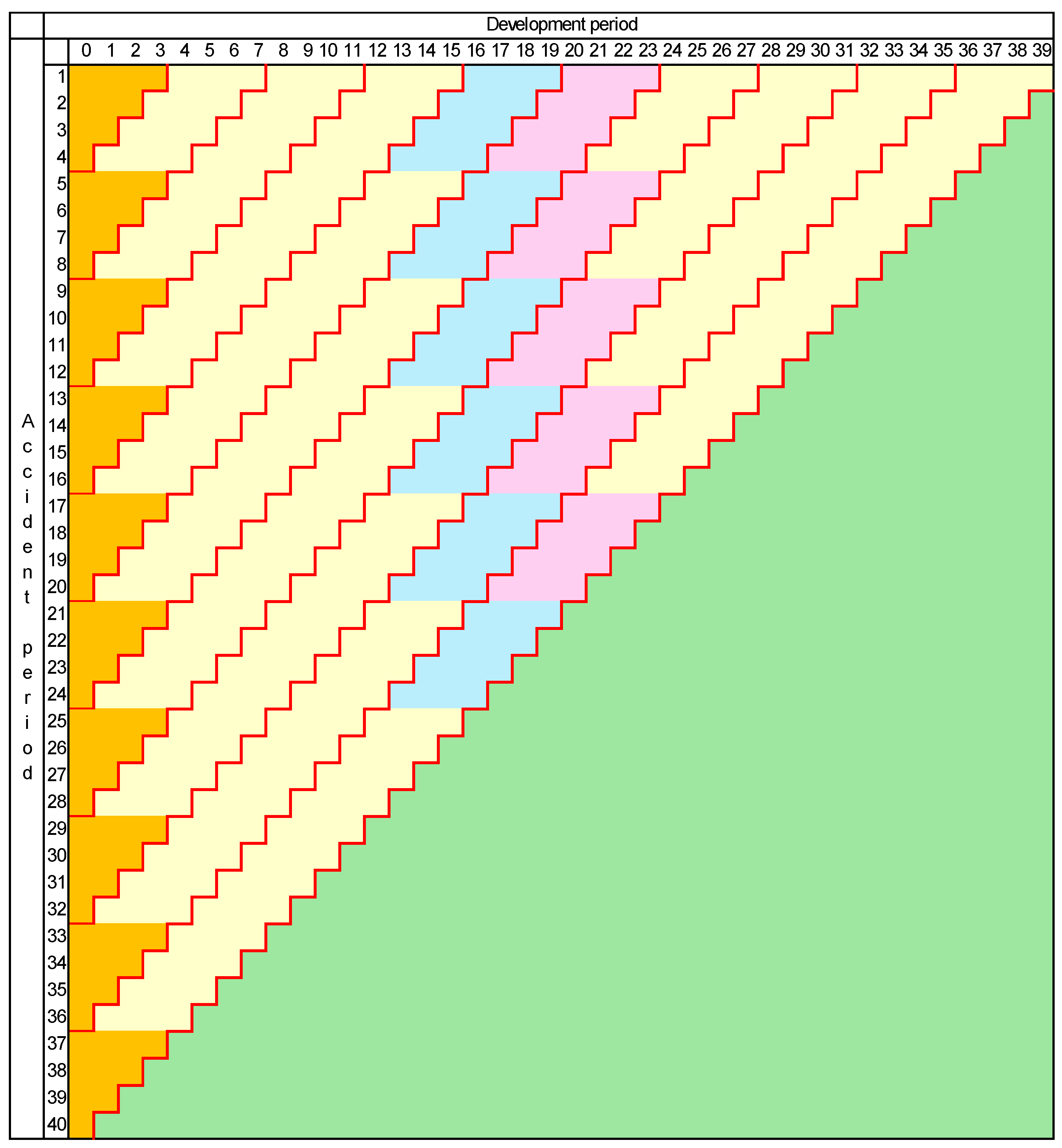
2.2.1. Preservation of Calendar Periods

Section 2.1 is phrased in terms of accident, development and calendar periods, without any specification of the meaning of “period”. Often, in the literature, this unit is a year. But it need not be; it might be a quarter, month, week, or any other convenient length of time. This will be referred to as the mesh size of the data triangle.

Consider how the mesh size might be changed. Suppose that, in ${\mathcal{D}}_U$, $I=Nq$ for some strictly positive integers $N,q$. The mesh size can be changed from one unit of time to $q$ units. There will then be $N$ accident and development periods, instead of the original $I$.

An example would be the case in which the units of time in ${\mathcal{D}}_U$ are quarters and $I=40,N=10,q=4$. Here, the mesh size is changed from quarters to years, and ${\mathcal{D}}_U$ contains 10 accident and development years.

In the case of general $N$ and $q$, the change of mesh will induce a new upper triangle ${\mathcal{D}}_U^{*}$ in which row $i^{*}$ will be obtained from the merger of rows $q\left(i^{*}-1\right)+1,q\left(i^{*}-1\right)+2,\dots ,q{i}^{*}$ from ${\mathcal{D}}_U$.

Now suppose, in addition, that the change of mesh is required to preserve calendar periods. By this is meant that calendar period $t^{*}$ in ${\mathcal{D}}_U^{*}$ will comprise calendar periods $q\left(t^{*}-1\right)+1,q\left(t^{*}-1\right)+2,\dots ,q{t}^{*}$ from ${\mathcal{D}}_U$.

For given $i^{\mathrm{*}}$ and $t^{\mathrm{*}}$, development period $j^{\mathrm{*}}=t^{\mathrm{*}}-i^{\mathrm{*}}$. Then the $\left(i^{\mathrm{*}},j^{\mathrm{*}}\right)$ cell of ${\mathcal{D}}_U^{\mathrm{*}}$ will consist of all pairs of $\left(q\left(i^{\mathrm{*}}-1\right)+r,\left[q\left(t^{\mathrm{*}}-1\right)+s\right]-\left[q\left(i^{\mathrm{*}}-1\right)+r\right]\right),r,s=1,\dots ,q$ from ${\mathcal{D}}_U$ such that the second member of the pair is non-negative. Equivalently, it consists of all pairs $\left(q\left(i^{\mathrm{*}}-1\right)+r,max\left[0,q{j}^{\mathrm{*}}+\left(s-r\right)\right]\right),r,s=1,\dots ,q$.

This is the form of aggregation from unit to $q$-unit periods commonly used in commercial practice. It is illustrated in Figure 1, in which a $40\times 40$ quarterly triangle is collapsed to a $10\times 10$ yearly triangle. The upper triangle is shaded yellow, the lower green. Calendar years are delineated by the red diagonals. Development years 5 and 6 are shaded blue and purple, respectively. Development year 0 is also shown orange to illustrate its exceptional nature.

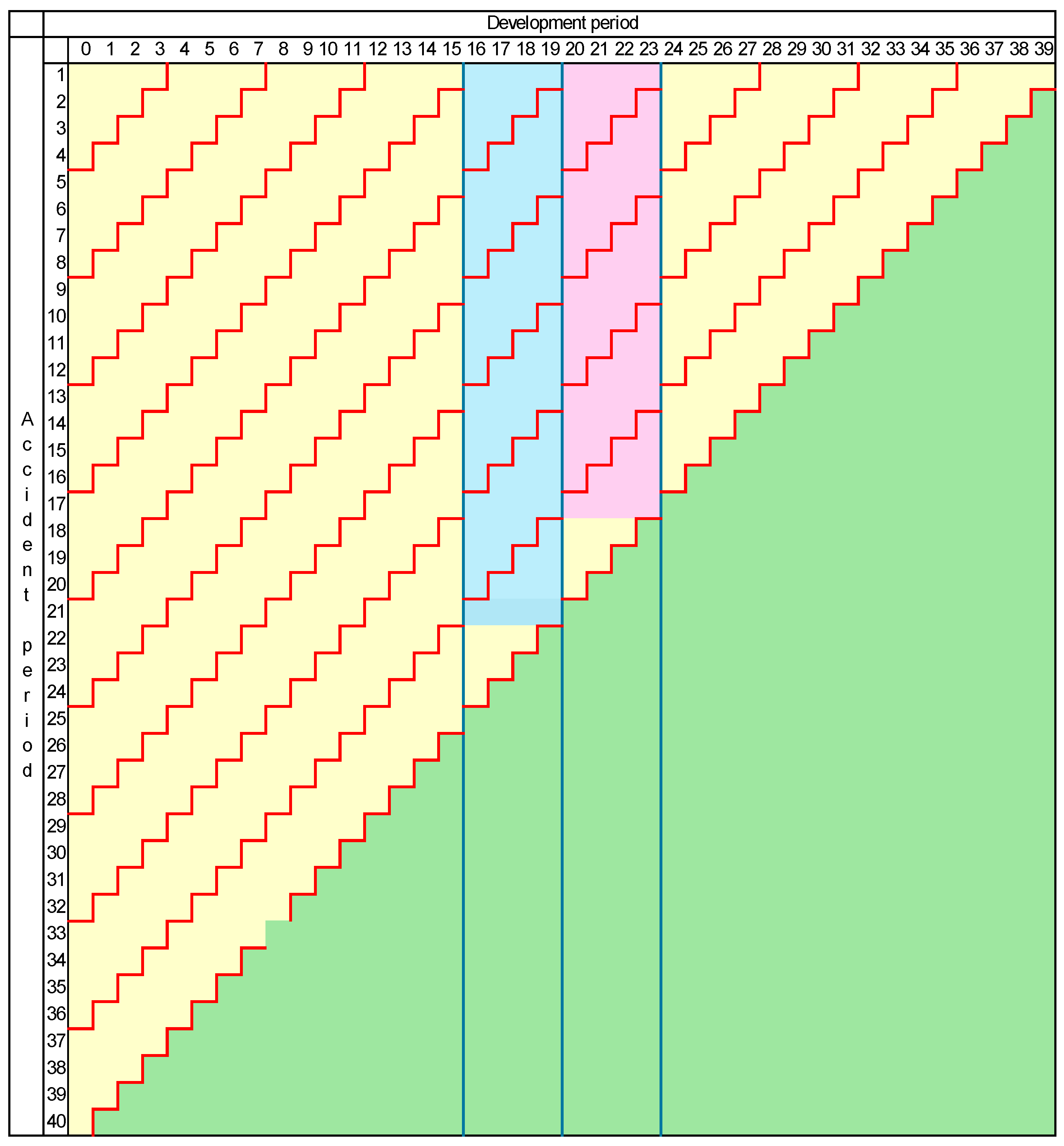
2.2.2. Preservation of Development Periods

It is seen in Figure 1 that the quarterly development periods that contribute to a specific yearly development period differ by accident quarter. Although this is standard commercial practice, one might regard this as undesirable. Indeed, Section 5.1 gives some justification for this view.

An alternative is as follows. Define merged accident periods exactly as in Section 2.2.1, but define merged development periods in such a way that development period $j^{*}$ always consists of the same development periods from ${\mathcal{D}}_U$.

In this case, there is no requirement that accident and development periods be subject to the mesh size. There is not even a requirement that all development periods be of the same duration. So partition the ordered set $\left\{0,\dots ,I\right\}$ by the insertion of cut-points $c_k,k=0,\dots ,K$ with $c_0=0,c_K=I$ so that $\left\{0,\dots ,I\right\}=\bigcup _{k=1}^K{S}_k$, where $S_k=\left\{{c_{k-1},\dots ,c}_k-1\right\}$. Then $S_k,k=1,\dots ,K$ become the merged development periods, where $S_k$ spans $c_k-c_{k-1}$ units of time.

The situation is illustrated in Figure 2, where development quarters 16 to 19 have been merged into a single development year, shaded blue; and similarly development quarters 20 to 23, shaded purple. The other development quarters have been left intact. Note that, for each of these development years, there is a triangle of data relating to the latest accident periods. These have not been shaded as they are incomplete and not comparable with the merged development years for earlier accident periods.

2.3. Sufficient Statistics

The present paper makes use of sufficient statistics in its argument. These and their properties are therefore briefly reviewed here. The review is general rather than specific to the context of the present paper.

Suppose that one makes observations $y_k,k=1,\dots ,K$ on some random variable $Y$ that depends on some generic parameter $\theta$, and let $T\left(y_1,\dots ,y_K\right)$ be an estimator of $\theta$. The general idea of a sufficient statistic for a parameter $\theta$ is that it contains all information relevant to the estimation of $\theta$. Thus, for example, if $T$ is sufficient for $\theta$, and is a dimension reducing mapping, i.e., $\dim T<K$, then there is no gain in information to be made by augmenting $T$ with any further detail from $y_1,\dots ,y_K$.

The following few sub-sections elaborate on the technical aspects of sufficient statistics, and how they relate to Generalized Linear Models (“GLMs”).

2.3.1. Sufficiency

Continue with the notation immediately above. Further, let the vector $y$ denote the sample of observations $\left\{y_1,\dots ,y_K\right\}$, and suppose that this vector is subject to the pdf $p\left(y;\theta \right)$.

Definition 1.

Let $T:S\to {\mathbb{R}}^M,M\le K$ for some ${S\subseteq \mathbb{R}}^K$. Then $T\left(y\right)$ is a sufficient statistic (Cox and Hinkley 1974) for $\theta$ if the conditional density $Prob\left\{y|T\left(y\right)\right\}$ is independent of $\theta$.

Note that $T$ reduces the data set of dimension $K$ to an $M$-dimensional random vector with $M\le K$. In the case $M<K$, the sufficient statistic $T$ will be said to be dimension-reducing.

A useful identification of sufficient statistics is given by the following result (Cox and Hinkley 1974).

Proposition 1.

(Fisher-Neyman factorization theorem). Let $T:S\to {\mathbb{R}}^M,M\le K$ for some ${S\subseteq \mathbb{R}}^K$. Then $T\left(y\right)$ is a sufficient statistic for $\theta$ if the density of $y$ can be decomposed in the following manner:

$$p\left(y;\theta \right)=f\left(y\right)g\left(T\left(y\right),\theta \right)$$

(8)

 for some non-negative functions $f$.

Some important estimation properties follow from sufficiency. The derivation of the first of these is elementary. Simply take logs throughout (8) and differentiate with respect to $\theta$, to obtain

$${\displaystyle \frac{\partial lnp\left(y;\theta \right)}{\partial \theta }}={\displaystyle \frac{\partial lng\left(T\left(y\right),\theta \right)}{\partial \theta }},$$

(9)

from which the following proposition is immediate.

Proposition 2.

Let $T\left(y\right)$ be a sufficient statistic for $\theta$ under the conditions of Definition 1. Assume further that $p\left(y;\theta \right)$ is differentiable with respect to $\theta$. Then the maximum likelihood estimator (“MLE”) of $\theta$ is a function of only $T\left(y\right)$.

Proof. 

The maximum likelihood (“ML”) equation sets (9) equal to zero. Since the right side of (9) involves only $T\left(y\right),\theta$, the MLE of $\theta$ must be a function of just $T\left(y\right)$. □

Sufficient statistics also lead to estimators of maximal efficiency (Lehmann and Scheffé 1950, 1955). This result requires the concept of completeness of a family of distributions.

Definition 2.

Consider the family of densities $\left\{p\left(y;\theta \right):\theta \in \Theta \right\}$ for some parameter space $\Theta$, and let $T\left(y\right)$ be a sufficient statistic for $\theta$. $T\left(y\right)$ is said to be complete if (Cox and Hinkley 1974), $E\left[q\left(T\right)|\theta \right]=0$ for every $q:{\mathbb{R}}^M\to \mathbb{R}$ only if $T\left(y\right)=0$ a.s.

Proposition 3.

(Lehmann-Scheffé). Let $\left\{p\left(y;\theta \right):\theta \in \Theta \right\}$ be a family of densities, and let $T\left(y\right)$ be a sufficient statistic for $\theta$ under the conditions of Definition 2.1. Let $T\left(y\right)$ be complete within the family, and suppose that $\psi$ is a mapping of $T\left(y\right)$ to $\Theta$, with the unbiased property $E\left[\psi \left(T\right)\right]=\theta$, where the expectation is taken over $Y_1,\dots ,Y_K$. Then $\psi \left(T\right)$ is the unique minimum-variance unbiased estimator (“MVUE”) of $\theta$.

2.3.2. Generalized Linear Models

The standard GLM (Nelder and Wedderburn 1972) takes the form

$$Y_i~EDF\left({\mu }_i,\phi \right),i=1,\dots ,n$$

(10)

with

$$\mu =E\left[Y\right]=h^{-1}\left(X\beta \right)$$

(11)

where

• the $Y_i$ are stochastically independent real-valued random variables, each with range $D$;
• $Y$ is the column $n$-vector with components $Y_i$;
• $EDF\left({\mu }_i,\phi \right)$ denotes a distribution from the exponential dispersion family (“EDF”) (Nelder and Wedderburn 1972) with mean ${\mu }_i$ and dispersion parameter $\phi ;$
• $\mu$ is the column $n$-vector with components ${\mu }_i$;
• $\beta$ is a column $p$-parameter;
• X is an $n\times p$ design matrix;
• $h:D\to R$ is an invertible function, called the link function, with $R$ a subset of the real line, and $h$ operating component-wise in (11).

The notations here are generic to GLMs and will take on different forms in the specific GLM of Section 3, Section 4 and Section 5. Observations $Y_{ij}$ in that specific model are doubly suffixed (instead of just $Y_i$ as in the generic description) and so the vector $Y$ there becomes the vector of all $Y_{ij}$. Similarly for other quantities such as $\mu$.

A distribution is a member of the EDF if its density takes the form (McCullagh and Nelder 1989)

$$p\left(y;\theta ,\phi \right)=exp\left\{{\displaystyle \frac{y\theta -b\left(\theta \right)}{a\left(\phi \right)}}+c\left(y,\phi \right)\right\}$$

for location and scale parameters $\theta ,\phi$ and some functions $a\left(.\right),b\left(.\right),c\left(.\right)$.

A member of the EDF is defined by its cumulant function $b$, a real-valued function of the real canonical parameter ${\theta }_i$ which is related to the mean ${\mu }_i$ by the relation ${\mu }_i=b\prime \left({\theta }_i\right)$. The link function is said to be canonical if $\theta =X\beta$, where $\theta$ is the vector of values ${\theta }_i$.

McCullagh and Nelder (1989, p. 32) point out an interesting and useful sufficient statistic of a GLM.

Proposition 4.

In the case of the GLM defined in (10) and (11), and provided that the link is canonical, $X^{T}Y$ is a sufficient statistic for $\beta$.

Note that $X^{T}Y$ is a $p$-vector, so of the same dimension as $\beta$.

A special case of the above GLM is obtained by restricting the EDF to its Tweedie sub-family (Tweedie 1984), for which the cumulant function is

$$b\left(\theta \right)={\displaystyle \frac{1}{2-p}}{\left[\left(1-p\right)\theta \right]}^{{\displaystyle \frac{2-p}{1-p}}}$$

(12)

for some parameter $pϵ\left(-\infty ,0\right]\cup [1,\infty )$.

A further special case is that in which $p=1$, and $b\left(\theta \right)=exp\theta ,a\left(\phi \right)=\phi$, obtained by allowing $p\uparrow 1$ in (12). This is the case of an over-dispersed Poisson (“ODP”) distribution. Note that, in this case,

$$expX\beta =b\prime \left(\theta \right)=exp\left(\theta \right)$$

(13)

where all functions operate on vectors component-wise. By definition, then, the log link function is canonical in this case. Specialization even further, with $\phi =1$, gives the Poisson case.

2.4. Notational Summary

For ease of reading the remainder of this paper,

Table 1. Summary of notation.

Symbol	Introduced in Section	Interpretation
$i$	Section 2.1	Accident period
$j$	Section 2.1	Development period
$t$	Section 2.1	Calendar period
$Y_{ij}$	Section 2.1	Amount of claim payments (random variable) made during development period $j$ of accident period $i$
$y_{ij}$	Section 2.1	Realization of the random variable $Y_{ij}$
${\mu }_{ij}$	Section 2.1	Mean of $Y_{ij}$
$Y$	Section 3.1	Vector of the $Y_{ij}$
${\mathcal{D}}_U$	Section 2.1	Upper triangle of observations (random variables) $Y_{ij}$
${\mathcal{D}}_L$	Section 2.1	Lower triangle of observations (random variables) $Y_{ij}$
${\mathcal{d}}_U$	Section 2.1	Realization of ${\mathcal{D}}_U$
$C_{ij}$	Section 2.1	Cumulative claim payments (random variable) corresponding to (non-cumulative) $Y_{ij}$
$c_{ij}$	Section 2.1	Realization of $C_{ij}$
${\mathcal{R}}_i$	Section 2.1	Row $i$ of upper triangle ${\mathcal{d}}_U$
${\mathcal{C}}_j$	Section 2.1	Column $j$ of upper triangle ${\mathcal{d}}_U$
$r_i$	Section 2.1	Row sum of ${\mathcal{d}}_U$ (over ${\mathcal{R}}_i$)
$s_j$	Section 2.1	Column sum of ${\mathcal{d}}_U$ (over ${\mathcal{C}}_j$)
$L_i$	Section 2.1	Amount of outstanding losses (the loss reserve) for accident period $i$
$L$	Section 2.1	Amount of outstanding losses (the loss reserve) for all accident periods
$i^{*},j^{*}$	Section 2.2	Accident and development periods under changed mesh size
${\mathcal{D}}_U^{*}$	Section 2.2	Upper triangle under changed mesh size
$\left\{c_0,\dots ,c_K\right\}$	Section 2.2.2	Partition of the interval $\left[0,I\right]$, defining development periods under changed mesh
${\alpha }_1,\dots ,{\alpha }_I,{\beta }_0,\dots ,{\beta }_{I-1}$	Section 3.1	EDF parameters for row and column effects in ${\mathcal{D}}_U$
$B_i$	Section 3.4.1	Loss reserve bias factor

summarizes both the notation introduced above and the main items of notation introduced in later sections. This necessarily involves forward references and these are noted in the table.

In addition, there are other notations (e.g., $y,\mu ,\theta$), occurring in Section 2.3.1 and Section 2.3.2, that relate to generic background results, and are not specific to the models used in Section 3 and subsequently. These have not been included in Table 1.

3. EDF Chain Ladder

3.1. Model Assumptions

The EDF chain ladder was discussed by Wüthrich and Merz (2008, Chapters 5 and 6). Taylor (2011) discussed the special case of the Tweedie chain ladder. It is the GLM defined by (10) to (12) and with the specific link function, observation vector, parameter vector and design matrix as follows:

$$h=ln$$

(14)

$${Y=\left(Y_{10},\dots ,Y_{1,I-1},Y_{20},\dots ,Y_{2,I-2},\dots ,Y_{I-1,0},Y_{I-1,1},Y_{I0}\right)}^T$$

(15)

$$\beta ={\left({\alpha }_1,\dots ,{\alpha }_I,{\beta }_0,\dots ,{\beta }_{I-1}\right)}^T$$

(16)

$$X=\left[\begin{array}{ccccc}{u}_I& & & & I_I\\ & u_{I-1}& & & I_{I-1}^{*}\\ & & \ddots & & ⋮\\ & & & u_1& I_1^{*}\end{array}\right]$$

(17)

Here the $Y_{ij}$ in (14) are the observations defined in Section 2.1, the ${\alpha }_i$ are the chain ladder row effects, the ${\beta }_j$ the column effects, and $I_i^{*}$ denotes the identity matrix $I_I$ with all but its first $i$ diagonal entries set to zero. As is well known, this model contains one degree of parameter redundancy, and so one linear constraint must be imposed on the $2I$ parameters if parameter estimation is to be carried out.

The vector $\mu$ of cell means ${\mu }_{ij}$ is given by $\mu =expX\beta$ and, by substitution of (16) and (17),

$${\mu }_{ij}=exp\left({\alpha }_i\right)exp\left({\beta }_j\right)$$

(18)

For $p=1$, the EDF chain ladder becomes the Poisson chain ladder.

3.2. Parameter Estimation

A GLM is typically calibrated by ML estimation, using GLM-specific software. However, Taylor (2011) shows that the ML equations for the Tweedie chain ladder take the simple form

$$\sum _{j\in {\mathcal{R}}_i}{\mu }_{ij}^{1-p}\left(y_{ij}-{\mu }_{ij}\right),i=1,\dots ,I,$$

(19)

$$\sum _{i\in {\mathcal{C}}_j}{\mu }_{ij}^{1-p}\left(y_{ij}-{\mu }_{ij}\right),j=0,\dots ,I-1.$$

(20)

In the Poisson chain ladder case, these ML equations reduce, by virtue of (18), to

$$exp\left({\alpha }_i\right)=r_i/\sum _{j\in {\mathcal{R}}_i}exp\left({\beta }_j\right),i=1,\dots ,I,$$

(21)

$$exp\left({\beta }_j\right)=s_j/\sum _{i\in {\mathcal{C}}_j}exp\left({\alpha }_i\right),j=0,\dots ,I-1.$$

(22)

3.3. Sufficient Statistics

Taylor (2011, Theorem 5.2) derives the following result.

Proposition 5.

For the Tweedie chain ladder defined in Section 3.1,

(a)

For $p\ne 1,$ the only sufficient statistic for any ${\alpha }_i$ or ${\beta }_j$ is the full data set ${\mathcal{D}}_U$; there is no sufficient statistic that is a proper subset of ${\mathcal{D}}_U$.

(b)

For $p=1$ (Poisson chain ladder), the set $\left\{r_1,\dots ,r_I,s_0,\dots ,s_{I-1}\right\}$ is a sufficient statistic for $\left\{{\alpha }_1,\dots ,{\alpha }_I,{\beta }_0,\dots ,{\beta }_{I-1}\right\}$.

Although Taylor proves this result by appeal to the Fisher-Neyman factorization theorem, it is interesting to note in passing that Proposition 5(b) can be obtained by substitution of (15) and (17) into Proposition 4 after taking note of the fact (Section 2.3.2) that the log link is canonical for the Poisson distribution. Thus,

$$X^{T}Y=\left[\begin{array}{cccc}{u}_I^T& & & \\ & u_{I-1}^T& & \\ & & \ddots & \\ & & & u_1^T\\ I_I& I_{I-1}^{*}& \dots & I_1^{*}\end{array}\right]\left[\begin{array}{c}\begin{array}{c}{Y}_1\\ Y_2\end{array}\\ \begin{array}{c}⋮\\ Y_I\end{array}\end{array}\right],$$

(23)

where $Y_i$ is the sub-vector of $Y$ that relates to row $i$ of the data set. Simple evaluation of the sufficient statistic $X^{T}Y$ then reveals it to be as claimed by Proposition 5(b).

A further result that will be found useful is the following, from Cox and Hinkley (1974).

Proposition 6.

Let $\left\{p\left(y;\theta \right):\theta \in \Theta \right\}$ be a family of EDF densities for specific cumulant function, and let $T\left(y\right)$ be a sufficient statistic for $\theta$ under the conditions of Definition 1. A necessary and sufficient condition that $T\left(y\right)$ be complete is that $dimT\left(y\right)=dim\theta$.

3.4. Forecast Bias

3.4.1. Poisson Case

As noted in Section 3.1, the parameters in Section 3.2 must be subject to a linear constraint. There are many possibilities but, for convenience, set

$$\sum _{j=0}^{I-1}exp\left({\beta }_j\right)=1,$$

(24)

in which case (21) may be re-expressed as

$$exp\left({\alpha }_i\right)=r_i/\left(1-\sum _{j=I-i+1}^{I-1}exp\left({\beta }_j\right)\right),i=1,\dots ,I.$$

(25)

In the case of the Poisson chain ladder, (22) and (25) provide an estimation algorithm if taken in the order $i=1,j=I-1,i=2,j=I-2,\dots ,j=0.$

For clarity of subsequent reasoning, it is desirable to re-state (22) and (25) in their random forms, as follows:

$$exp\left({\widehat{\alpha }}_i\right)=R_i/\left(1-\sum _{j=I-i+1}^{I-1}exp\left({\widehat{\beta }}_j\right)\right),i=1,\dots ,I.$$

(26)

$$exp\left({\widehat{\beta }}_j\right)=S_j/\sum _{i\in {\mathcal{C}}_j}exp\left({\widehat{\alpha }}_i\right),j=0,\dots ,I-1.$$

(27)

where $R_i,S_j$ are the random variables of which $r_i,s_j$ are realizations, and ${\widehat{\alpha }}_i,{\widehat{\beta }}_j$ are the estimates of ${\alpha }_i,{\beta }_j$.

The above recursive computation of the estimates indicates that they are explicit functions (albeit of a complicated nature) of the random variables $R_i,S_j$, which are Poisson variates with means that depend explicitly on the set of parameters ${\alpha }_i,{\beta }_j$. By (18), future values of $C_{ij}$ are forecast by ${\widehat{C}}_{ij}=exp\left({\widehat{\alpha }}_i\right)exp\left({\widehat{\beta }}_j\right)$, and so, by (5) and (7), ${\widehat{L}}_i$ and $\widehat{L}$ are also explicit functions of these Poisson variates. Write ${\widehat{L}}_i={\lambda }_i\left(\widehat{\alpha },\widehat{\beta }|\alpha ,\beta \right),\widehat{L}=\lambda \left(\widehat{\alpha },\widehat{\beta }|\alpha ,\beta \right)$, where the true parameters $\alpha ,\beta$ are unknown.

For given parameters $\alpha ,\beta ,$ the expectation of the estimated loss reserves is

$$E\left[{\widehat{L}}_i\right]=E_{{\mathcal{D}}_U}\left[{\lambda }_i\left(\widehat{\alpha },\widehat{\beta }|\alpha ,\beta \right)\right].$$

(28)

The chain ladder forecast is conventionally taken as just ${\widehat{L}}_i={\lambda }_i\left(\widehat{\alpha },\widehat{\beta }|\alpha ,\beta \right)$, and so the bias in this estimator might be taken as the ratio of $E\left[{\widehat{L}}_i\right]$ to $E\left[L_i\right]$. Unfortunately, the latter is not calculable because $\alpha ,\beta$ in (28) are unknown. An alternative estimate of bias can be obtained by comparison between ${\widehat{L}}_i$ and ${E\left[{\widehat{\widehat{L}}}_i\right]=E}_{{\mathcal{D}}_U}\left[{\lambda }_i\left(\widehat{\widehat{\alpha }},\widehat{\widehat{\beta }}|\left(\widehat{\alpha },\widehat{\beta }\right)\right)\right]$, where $\widehat{\widehat{\alpha }},\widehat{\widehat{\beta }}$ are the estimates of the chain ladder parameters from a data triangle ${\mathcal{D}}_U$ randomly sampled from parameters $\widehat{\alpha },\widehat{\beta }$.

The (estimated) chain ladder bias factor is then $B_i={\widehat{L}}_i/E\left[{\widehat{\widehat{L}}}_i\right]$. A similar factor $B$ can be calculated as the bias associated with $\widehat{L}$.

3.4.2. General EDF Case

Bias in the general EDF case can be estimated in a similar way, but with one variation. The need for this arises from the fact that the ML Equations (19) and (20) do not yield explicit solutions for $\alpha ,\beta$.

An iterative solution is suggested by Taylor (2009), in which (19) and (20) are replaced by

$$\sum _{j\in {\mathcal{R}}_i}{\left({\mu }_{ij}^{\left(m\right)}\right)}^{1-p}\left(y_{ij}-{\mu }_{ij}^{\left(m+1\right)}\right),i=1,\dots ,I,$$

(29)

$$\sum _{i\in {\mathcal{C}}_j}{\left({\mu }_{ij}^{\left(m\right)}\right)}^{1-p}\left(y_{ij}-{\mu }_{ij}^{\left(m+1\right)}\right),j=0,\dots ,I-1,$$

(30)

for $m=0,1,\dots$, where ${\mu }_{ij}^{\left(m\right)}={\alpha }_i^{\left(m\right)}{\beta }_j^{\left(m\right)}$ is the $m$-th iterate on the estimate of ${\mu }_{ij}$.

In this schema, at each $m$, (29) and (30) are solved for ${\alpha }_i^{\left(m+1\right)}{,\beta }_j^{\left(m+1\right)}$ with values of ${\mu }_{ij}^{\left(m\right)}$ fixed by the preceding iteration. The procedure is initiated by some convenient selection of ${\alpha }_i^{\left(0\right)}{,\beta }_j^{\left(0\right)}$, possibly the Poisson chain ladder solution (21) and (22), and continued until successive iterates of the ${\alpha }_i^{\left(m\right)}{,\beta }_j^{\left(m\right)}$ are sufficiently close that convergence may be assumed.

Convergence may or may not occur. It might occur, but there might be multiple solutions. Taylor (2017) gives an example of a triple solution for an inverse Gaussian distribution (Tweedie, $p=3$). In such cases, bias correction cannot be obtained by these means.

Bias factors may be derived just as in Section 3.4.1.

3.5. Forecast Variance

Consider the estimator ${{\mathcal{L}}_i=\widehat{L}}_i/B_i$, where $B_i$ is the bias factor derived in Section 3.4.1 (and which is similarly applicable to Section 3.4.2). It is evident that ${\mathcal{L}}_i$ is an unbiased estimator of $L_i$.

3.5.1. Poisson Case

Proposition 7.

Consider the Poisson chain ladder model of Section 3.1. The bias-corrected reserve estimators ${\mathcal{L},\mathcal{L}}_i$ defined in Section 3.4.1 are unique MVUEs.

Proof. 

It is evident from (21) and (22) that the estimates of the parameters $\alpha ,\beta$ are functions of the summary statistics $\left\{r_1,\dots ,r_I,s_0,\dots ,s_{I-1}\right\}$ which, by Proposition 5, form a sufficient statistic $T\left({\mathcal{D}}_U\right)$. Hence $\widehat{L},{\widehat{L}}_i$ are functions of this sufficient statistic. □

From Section 3.4.1, the bias factors ${B,B}_i$ are functions of the parameter estimates $\widehat{\alpha },\widehat{\beta }$, and therefore functions of the sufficient statistic $T\left({\mathcal{D}}_U\right)$. It then follows that the bias-corrected loss reserve estimates ${\mathcal{L}}_i,\mathcal{L}\left(=\sum _i{\mathcal{L}}_i\right)$ are functions of $T\left({\mathcal{D}}_U\right)$.

It remains to check that $T\left({\mathcal{D}}_U\right)$ is complete. This can be demonstrated with the help of Proposition 6. Note that, as written, $T\left({\mathcal{D}}_U\right)$ has dimension $2I$, and this is a sufficient statistic for ${\left[{\alpha }^T,{\beta }^T\right]}^T$, which also has dimension $2I$.

However, it has been noted in Section 3.1 that this parameter vector has in fact only $2I-1$ independent components. Moreover, it may also be noted that the components of $T\left({\mathcal{D}}_U\right)$ are also not independent. This can be seen from the fact that

$$r_1+\dots +r_I=s_0+\dots +s_{I-1}={\sum }_{{\mathcal{D}}_U}{Y}_{ij}$$

(31)

the sum of all observations.

Thus, it is more useful to regard ${\left[r_1,\dots ,r_{I-1},s_0,\dots ,s_{I-1}\right]}^T$, of dimension $2I-1$, as a sufficient statistic for ${\left[{\alpha }_1,\dots ,{\alpha }_{I-1},{\beta }_0,\dots ,{\beta }_{I-1}\right]}^T$, also of dimension $2I-1$. The equality of these two dimensions, together with Proposition 6, then guarantees that $T\left({\mathcal{D}}_U\right)$, or its abbreviated form, is a complete sufficient statistic.

All conditions of Proposition 3 are now satisfied, justifying the stated result.

The discussion hitherto has been confined to the Poisson case for the sake of simplicity. However, Taylor’s result (Taylor 2011, Theorem 5.2), cited earlier as relating to the Poisson case, actually applies to the more general ODP case. Here, for known scale parameter $\phi$, the above sufficient statistic for the Poisson case remains sufficient for the ODP case. Hence the following remark.

Remark 1.

Proposition 7 applies equally to the ODP chain ladder with known scale parameter $\phi$.

Remark 2.

Further, it is well known that the magnitude of the scale parameter has no effect on the GLM’s parameter estimates, but all variance estimates are proportional to it.

3.5.2. General EDF Case

Now consider the general EDF chain ladder model of Section 3.1. In this case, as noted by Proposition 5(a), for $p\ne 1,$ there is no sufficient statistic for the parameter set that is a proper subset of ${\mathcal{D}}_U$. One can, of course, choose $T\left({\mathcal{D}}_U\right){=\mathcal{D}}_U$ as the sufficient statistic.

The bias-corrected reserve estimates ${\mathcal{L},\mathcal{L}}_i$ are evidently functions of this sufficient statistic. However, $T\left({\mathcal{D}}_U\right)$ is not complete, since $dimT\left({\mathcal{D}}_U\right)=½I\left(I+1\right)$, which is not equal to the dimension of the parameter vector ${\left[{\alpha }_1,\dots ,{\alpha }_{I-1},{\beta }_0,\dots ,{\beta }_{I-1}\right]}^T$. The sufficient statistic therefore fails the completeness test, according to Proposition 6.

As a result, Proposition 3 cannot be invoked. This does not prove that the reserve estimates ${\mathcal{L},\mathcal{L}}_i$ are not MVUE, but it does leave the question open.

4. Effects of Change of Mesh Size Under Preservation of Calendar Periods

4.1. Model Assumptions

4.1.1. EDF Chain Ladder

Consider a given claim data set ${\mathcal{D}}_U$ and the imposition on it of a larger mesh size, as described in Section 2.2.1. It is commonly assumed that one can make such changes at will while retaining an EDF chain ladder model. This assumption, however, warrants consideration.

Cells under the enlarged mesh are obtained by simple addition of the cells of smaller mesh, but note that the EDF is not closed under addition of random variables except under restrictive conditions. These are given for the Tweedie sub-family by Taylor (2021, Theorem 2.5), which leads to the following result.

Proposition 8.

Consider a claim data set ${\mathcal{D}}_U$ for which all observations are Tweedie distributed with Tweedie parameter $p$. Then observations under increased mesh size remain Tweedie distributed if and only if one of the following two conditions holds:

(a)

All observations are normally distributed ($p=0$); or

(b)

All observations have common ratio of mean to variance.

If these conditions are not satisfied, one is not strictly entitled to apply the EDF (or, more particularly, Tweedie) chain ladder to the data set with increased mesh.

4.1.2. Poisson Chain Ladder

Proposition 9.

(special case of Proposition 8). A data set of Poisson observations remains so under enlargement of mesh size.

Proof. 

The Poisson family of distributions satisfies condition (b) of Proposition 8. Specifically, the ratio of mean to variance is unity. The stated result is therefore a special case of Proposition 8. □

4.1.3. Structure of Cell Means

The Poisson chain ladder model of Section 3.1 requires not only Poisson distributions for all observations, but also that cell means assume the form (18). It is necessary to check whether this structure remains after mesh enlargement. The situation is, in fact, as set out in Proposition 10 below.

For the purpose of just this section, adopt the notation

$$a_i=exp{\alpha }_i,b_j=exp{\beta }_j$$

(32)

so the required cell structure (18) can be expressed in the form

$${\mu }_{ij}=a_i{b}_j$$

(33)

Further, for given integer $q>1$, define

$${\xi }_{q{j}^{*}-k}={\sum }_{\mathcal{l}=1}^q{b}_{q{j}^{*}+\left(\mathcal{l}-k\right)}$$

(34)

and

$${\rho }_{q{j}^{*}-k}={\displaystyle \frac{{\xi }_{q\left(j^{*}+1\right)-k}}{{\xi }_{q{j}^{*}-k}}}.$$

(35)

Then introduce the matrix and vector notation

$$\begin{array}{l}{w}_{i^{*}}={\left[a_{q\left(i^{*}-1\right)+1},\dots ,a_{q\left(i^{*}-1\right)+q}\right]}^T,v_{j^{*}}={\left[{\xi }_{q{j}^{*}-1},\dots ,{\xi }_{q{j}^{*}-q}\right]}^T,\\ \hspace{1em}\hspace{1em}\hspace{1em}{D}_{j^{*}}=diag\left({\rho }_{q{j}^{*}-1},\dots ,{\rho }_{q{j}^{*}-q}\right),M_{j^{*}}=D_{j^{*}}{v}_{j^{*}}{v}_{j^{*}}^T-v_{j^{*}}{v}_{j^{*}}^T{D}_{j^{*}}\end{array}$$

(36)

Proposition 10.

Let ${\mathcal{D}}_U$ be a data triangle satisfying the conditions for which a Poisson chain ladder model is valid, i.e.,  $Y_{ij}~Poisson\left({\mu }_{ij}\right)$, with ${\mu }_{ij}$ taking the form (18). Now increase the mesh size of the triangle by a factor $q$, preserving calendar periods (as illustrated in  Section 2.2.1). A necessary and sufficient condition for the Poisson chain ladder to be a valid model for the triangle with enlarged mesh is that, for all choices of $i^{*},i^{**},$

$$w_{i^{*}}^T{M}_{j^{*}}{w}_{i^{**}}=0,j^{*}\ge 1,$$

(37)

 in the above notation, with a similar but slightly different requirement for the case $j^{*}=0.$

Proof. 

A different characterization of this structure, which follows from and implies (18), is

$${\displaystyle \frac{{\mu }_{i,j+1}}{{\mu }_{ij}}}={\displaystyle \frac{b_{j+1}}{b_j}},\mathrm{i}\mathrm{n}\mathrm{d}\mathrm{e}\mathrm{p}\mathrm{e}\mathrm{n}\mathrm{d}\mathrm{e}\mathrm{n}\mathrm{t}\mathrm{o}\mathrm{f}i.$$

(38)

Now consider this requirement under mesh enlargement by a factor of $q$ as set out in Section 2.2.1. In the notation established there, the left side of (38) is replaced, in the case ${,j}^{*}\ge 1$, by

$${\displaystyle \frac{{\mu }_{i^{*}{,j}^{*}+1}}{{\mu }_{i^{*}{,j}^{*}}}}={\displaystyle \frac{\sum _{k=1}^q\left(a_{q\left(i^{*}-1\right)+k}{\sum }_{\mathcal{l}=1}^q{b}_{q\left(j^{*}+1\right)+\left(\mathcal{l}-k\right)}\right)}{\sum _{k=1}^q\left(a_{q\left(i^{*}-1\right)+k}{\sum }_{\mathcal{l}=1}^q{b}_{q{j}^{*}+\left(\mathcal{l}-k\right)}\right)}}={\displaystyle \frac{\sum _{k=1}^q{a}_{q\left(i^{*}-1\right)+k}{{\rho }_{q{j}^{*}-k}\xi }_{q{j}^{*}-k}}{\sum _{k=1}^q{a}_{q\left(i^{*}-1\right)+k}{\xi }_{q{j}^{*}-k}}}.$$

(39)

This may be abbreviated by use of the matrix and vector notation above, thus

$${\displaystyle \frac{{\mu }_{i^{*}{,j}^{*}+1}}{{\mu }_{i^{*}{,j}^{*}}}}={\displaystyle \frac{w_{i^{*}}^T{D_{j^{*}}v}_{j^{*}}}{w_{i^{*}}^T{v}_{j^{*}}}}.$$

(40)

In parallel with (38), it is required that, for each $j^{*}\ge 1,$ the ratio immediately above be independent of $i^{*}$. Equivalently, for $i^{*},i^{**}=1,\dots ,I,$

$${\displaystyle \frac{w_{i^{*}}^T{D_{j^{*}}v}_{j^{*}}}{w_{i^{*}}^T{v}_{j^{*}}}}={\displaystyle \frac{w_{i^{**}}^T{D_{j^{*}}v}_{j^{*}}}{w_{i^{**}}^T{v}_{j^{*}}}},j^{*}\ge 1.$$

(41)

For conciseness, it will be convenient to drop the subscript $j^{*}$, cross-multiply in the last equation, and rearrange slightly, to obtain

$$w_{i^{*}}^T\left(Dv{v}^T\right)w_{i^{**}}=w_{i^{*}}^T\left(v{v}^{T}D\right)w_{i^{**}}$$

(42)

which, by (36), is the same as (37). □

Remark 3.

It is straightforward to check that $M_{j^{*}}$ is a $q\times q$ matrix with $\left(k,\mathcal{l}\right)$ element $\left({\rho }_{q{j}^{*}-k}-{\rho }_{q{j}^{*}-\mathcal{l}}\right){\xi }_{q{j}^{*}-k}{\xi }_{q{j}^{*}-\mathcal{l}},k,\mathcal{l}=1,\dots ,q$. It is thus anti-symmetric. It immediately follows that $w_{i^{*}}^T{M}_{j^{*}}{w}_{i^{*}}=0$ in (37), as it must.

The condition (37) is very restrictive, but there are some simple conditions under which it is satisfied.

Corollary 1.

Each of the following conditions is sufficient for the satisfaction of (37):

(a)

$D_{j^{*}}$ is a scalar matrix, i.e., ${\rho }_{q{j}^{*}-1}={\rho }_{q{j}^{*}-2}=\dots {\rho }_{q{j}^{*}-q}$;

(b)

$w_{i^{**}}=C{w}_{i^{*}}$ for some constant $C>0$.

Proof of Corollary 1.

Combine condition (a) with Remark 3 to obtain $M_{j^{*}}=0$, whence (37) is satisfied.

Under condition (b), $w_{i^{\mathrm{*}}}^T{M}_{j^{\mathrm{*}}}{w}_{i^{\mathrm{*}\mathrm{*}}}^T=C{w}_{i^{\mathrm{*}}}^T{M}_{j^{\mathrm{*}}}{w}_{i^{\mathrm{*}}}^T=0$, by Remark 3. □

Remark 4.

The meaning of condition (a) of the corollary is that, within each development period under the enlarged mesh, the ratio of expected claim payments in one of the component unenlarged development periods to the expected payments in the corresponding component of the previous enlarged development period is independent of the component chosen.

The meaning of condition (b) is that each accident period under the enlarged mesh is distributed in proportions over its component accident periods from the unenlarged mesh in the same way as every other accident period.

4.2. Forecast Variance

Consider a model with enlarged mesh that jumps all the hurdles of Section 4.1, i.e., it is a Poisson chain ladder model that satisfies (37) under an enlargement of mesh size. Then, by Proposition 10, it remains a Poisson chain ladder model under the enlarged mesh. A question arises as to which mesh size produces the most efficient forecast of loss reserve.

By Proposition 7, application of the chain ladder algorithm to ${\mathcal{D}}_U$ (unenlarged mesh) produces a unique MVUE estimate of loss reserve for that data set. As seen in Section 2.2.1, each cell of the upper triangle ${\mathcal{D}}_U^{*}$ induced by the change of mesh size is obtained by summation of cells of ${\mathcal{D}}_U$.

The row and column sums of ${\mathcal{D}}_U^{*}$ are a sufficient statistic for ${\mathcal{D}}_U^{*}$ when the available data comprise the latter. However, they are not a sufficient statistic for ${\mathcal{D}}_U$ when those more granular data are available. This result is summarized as follows.

Proposition 11.

Consider a Poisson chain ladder model on data triangle ${\mathcal{D}}_U$, and subject this triangle to the increase in mesh size described in Section 2.2.1. Suppose that condition (37) in Proposition 10 is satisfied, in which case the induced data triangle ${\mathcal{D}}_U^{*}$ is also described by a Poisson chain ladder model.

Then

(a)

$Var\left[\widehat{L}|{\mathcal{D}}_U\right]$ is the unique MVUE of all unbiased estimators of $L$, so conditioned;

(b)

$Var\left[{\widehat{L}}^{*}|{\mathcal{D}}_U^{*}\right]$ is the unique MVUE of all unbiased estimators of $L$, so conditioned;

(c)

$Var\left[\widehat{L}|{\mathcal{D}}_U\right]<Var\left[{\widehat{L}}^{*}|{\mathcal{D}}_U^{*}\right]$.

Proof. 

Proposition 5(b) defines the (different) sufficient statistics for the respective model parameters in the two cases of data triangle. The sufficient statistic defines an MVUE forecast of loss reserve in each of the cases of ${\mathcal{D}}_U$ and ${\mathcal{D}}_U^{*}$. Denote these forecasts by $\widehat{L}$ and ${\widehat{L}}^{*}$, respectively. Then the proposition follows. □

In other words, subject to the sustained validity of a Poisson chain ladder model, the bias-corrected chain ladder forecast of a loss reserve is always improved by increased granularity, subject to preservation of diagonals.

5. Effects of Change of Mesh Size Under Preservation of Development Periods

5.1. Model Assumptions

5.1.1. EDF and Poisson Chain Ladder

Consider a given claim data set ${\mathcal{D}}_U$ and the imposition on it of a larger mesh size, as described in Section 2.2.2. Propositions 8 and 9 continue to hold. The supporting arguments are as in Section 4.1.1 and Section 4.1.2.

5.1.2. Structure of Cell Means

It was seen in Section 4.1.3 that the validity of a Poisson chain ladder model continued to hold under mesh enlargement with preservation of calendar periods only under restrictive conditions on the chain ladder parameters of the smaller-mesh model. It is of interest to consider the conditions under which a Poisson chain ladder model remains valid when the mesh is enlarged with preservation of development periods, as in Section 2.2.2.

Consider the Poisson chain ladder model of Section 3.1 and, again, temporarily adopt the notation of (32) and (33). Now, in the notation of Section 2.2.2, define development period $j^{*}$ under a mesh enlargement to be the merged period $S_{j^{*}}$.

Accident periods $1,\dots ,I$ can be partitioned in any way desired, so let a new accident period $i^{*}$ under mesh enlargement comprise accident periods $h_{i^{*}},h_{i^{*}}+1,\dots ,h_{i^{*}}+d_{i^{*}}-1$ under the unenlarged mesh. Here accident period $i^{*}$ spans $d_{i^{*}}$ of the original time units. The question arises as to the extent to which cells remain Poisson distributed under this re-definition of development periods. The next result answers this question.

Proposition 12.

Let ${\mathcal{D}}_U$ be a data triangle satisfying the conditions for which a Poisson chain ladder model is valid, i.e.,  $Y_{ij}~Poisson\left({\mu }_{ij}\right)$ , with ${\mu }_{ij}$ taking the form (18). Now increase the mesh size of the triangle, preserving development periods (as illustrated in Section 2.2.2). The Poisson chain ladder continues to be a valid model for all cells of the triangle with enlarged mesh except the edge cells defined in the proof below.

Proof. 

The expected value of payments in cell $\left(i^{*},j^{*}\right)$ under the new mesh is

$${\mu }_{i^{*}{,j}^{*}}=\sum _{k=0}^{d_{i^{*}}-1}\sum _{\mathcal{l}=c_{j^{*}-1}}^{c_{j^{*}}-1}{a_{h_{i^{*}}+k}b}_{\mathcal{l}}=\left(\sum _{k=0}^{d_{i^{*}}-1}{a}_{h_{i^{*}}+k}\right)\left(\sum _{\mathcal{l}=c_{j^{*}-1}}^{c_{j^{*}}-1}{b}_{\mathcal{l}}\right),$$

(43)

provided that none of the cells $\left(h_{i^{*}}+k,c_{j^{*}-1}\right)$ lies outside the triangle ${\mathcal{D}}_U$, i.e., provided that $\left(h_{i^{*}}+d_{i^{*}}-1\right)+\left(c_{j^{*}}-1\right)\le I$.

Relation (43) is of the form (18). Just as in Proposition 9, the amount of claim payments in cell $\left(i^{*},j^{*}\right)$, as the sum of Poisson variates, is Poisson.

If the constituent cells do not all lie within ${\mathcal{D}}_U$, then the factorization in (43) occurs only if $d_{i^{*}}=1$ (no aggregation of accident periods) or the trivial case $c_{j^{*}}=c_{j^{*}-1}$ (no aggregation of development periods). Call these cells edge cells. They are exemplified in Figure 2, where they are bordered by the $I$-th diagonal in ${\mathcal{D}}_U$, the most recent past diagonal. □

Note that the edge cells are incomplete in the sense that they include fewer of the smaller-mesh cells than is the case for earlier accident periods, and so are not comparable with any larger-mesh development period from earlier accident periods.

It is supposed here that one makes a decision as to the granularity of collected data, after which data of greater granularity are unavailable. There are two alternative ways forward. Either:

• formulate a model of the incomplete larger-mesh development periods (which will not be informed by more granular data); or
• exclude the edge cells from the data set as uninformative.

The first alternative is viable. For example, one might assume that claim payments occur uniformly over the larger-mesh development periods, or according to some other convenient distribution. However, the resulting model, while perfectly respectable, would no longer be chain ladder, and so is not pursued here.

In the second case, the edge cells are deleted from the upper triangle, and regarded as belonging to the future, therefore requiring forecast. The situation is illustrated by Figure 3, which is a replica of Figure 2 except that edge cells have been marked in green as belonging to the future.

In this figure, development quarters 16 to 19 have been merged into a single development year, as in Figure 2, and similarly for development quarters 20 to 23. The figure also indicates that accident quarters 17 to 24 are to be merged into four accident half-years.

The general situation is summarized by the following statement.

Proposition 13.

Let ${\mathcal{D}}_U$ be a data triangle satisfying the conditions for which a Poisson chain ladder model is valid, i.e., $Y_{ij}~Poisson\left({\mu }_{ij}\right)$, with ${\mu }_{ij}$ taking the form (18). Now increase the mesh size of the triangle for certain accident and development periods, preserving development periods (as illustrated in Section 2.2.2). The mesh-enlarged development periods need not be of equal lengths, nor need the mesh-enlarged accident periods. There need be no relation between the lengths of mesh-enlarged accident and development periods. Define ${\mathcal{D}}_U^{*}$ to be the data set induced on ${\mathcal{D}}_U$ by the mesh enlargement, and let ${\mathcal{D}}_U^{*(-)}$ be the data set obtained by the deletion of edge cells from ${\mathcal{D}}_U^{*}$. Then a Poisson chain ladder model remains valid on ${\mathcal{D}}_U^{*(-)}$.

Proof. 

A Poisson chain ladder model can be applied to the data set ${\mathcal{D}}_U^{*(-)}$ (in the above example, this consists of the part of Figure 3 not shaded green and not forming the incomplete accident half-years comprising accident quarters 17 and 21). The model is simply

$$Y_{i^{*}{j}^{*}}~Poisson\left({\mu }_{i^{*}{j}^{*}}\right)$$

(44)

$${\mu }_{i^{*}{j}^{*}}=exp\left({\alpha }_{i^{*}}\right)exp\left({\beta }_{j^{*}}\right)$$

(45)

(compare (18)) where the cells of ${\mathcal{D}}_U^{*(-)}$ are labelled $\left(i^{*},j^{*}\right)$ with $i^{*},j^{*}$ labelling the accident and development periods under the enlarged mesh.

This chain ladder model will forecast the ultimate cost of each mesh-enlarged accident period. Total payments up to the valuation date are known for each of these accident periods, and so the outstanding liability for each accident period can be inferred. □

5.2. Forecast Variance

Consider the model and mesh enlargement described in Proposition 12. As in Section 4.2, a question arises as to which mesh size produces the most efficient forecast of loss reserve. This question is answered by logic parallel to that applied in Section 4.2, leading to the following result.

Proposition 14.

Consider a Poisson chain ladder model on data triangle ${\mathcal{D}}_U$, and subject this triangle to an increase in mesh size described in Section 2.2.2. Then the induced data triangle ${\mathcal{D}}_U^{*(-)}$ is also described by a Poisson chain ladder model.

Proposition 5(b) defines the (different) sufficient statistics for the respective model parameters in the two cases of data triangle. The sufficient statistic defines a unique MVUE forecast of loss reserve in each of the cases of ${\mathcal{D}}_U$ and ${\mathcal{D}}_U^{*(-)}$. Denote these forecasts by $\widehat{L}$ and ${\widehat{L}}^{*(-)}$, respectively.

Then

(a)

$Var\left[\widehat{L}|{\mathcal{D}}_U\right]$ is the unique minimum variance of all unbiased estimators of $L$, so conditioned;

(b)

$Var\left[{\widehat{L}}^{*(-)}|{\mathcal{D}}_U^{*\left(-\right)}\right]$ is the unique minimum variance of all unbiased estimators of $L$, so conditioned;

(c)

$Var\left[\widehat{L}|{\mathcal{D}}_U\right]<Var\left[{\widehat{L}}^{*(-)}|{\mathcal{D}}_U^{*(-)}\right]$.

6. Numerical Example

A simple numerical example is given to illustrate the result in Proposition 14. It is based on the synthetic data triangle set out in

Table 2. Data Triangle For Numerical Example.

Accident	Claim Payments in Development Year
Year	0	1	2	3	4	5	6	7	8	9
1	5840	15,169	10,338	7518	5954	4451	2967	2135	1123	593
2	6205	15,311	10,682	7552	6080	4608	2990	2188	1185
3	6254	15,915	11,107	8035	6217	4705	3130	2172
4	6349	16,180	11,272	7999	6375	4908	3193
5	7011	17,559	12,396	8967	7108	5272
6	6755	17,464	12,180	8787	7061
7	7277	18,481	12,511	9212
8	7525	18,714	13,134
9	7508	19,019
10	7834

, which is deliberately constructed as well behaved and consistent with the chain ladder structure set out in (18).

Initially in the example, development years 3 and 4 are merged, just as two consecutive development periods are merged in the theoretical workings of Section 5. This is reflected in the blue shading in the table. In addition, cell (7,3) is shaded brown to indicate that there is no corresponding value in cell (7,4) with which it can be merged, whereas a combined “development years 3 and 4” cell can be formed for each of accident years 1 to 6, and used in chain ladder modelling of this combination, cell (7,3) is unusable in the modelling.

Call the triangle in the Table 2 the unmerged triangle, and apply the name “merged triangle” to the new version in which development years 3 and 4 are merged into a single “3 and 4” development period. The Poisson chain ladder is applied to each, on the basis of Section 3 in the unmerged case and Section 5 in the merged case. The latter of these is achieved by eliminating development year 3 and cell (7,3) from the design matrix $X$ in (17).

In each case, the outstanding losses are forecast and the variance of this forecast calculated from the relevant GLM. The calculation follows (Wüthrich and Merz 2008, Section 6.4, especially (6.47) and Lemma 6.13). The results are as set out in

Table 3. Forecasts And Standard Deviations Of Forecasts For Merged And Unmerged Data Triangles.

Accident	Forecast Outstanding Losses		Standard Deviation of Forecast
Year
	Unmerged	Merged	Unmerged	Merged
2	607	607	25	25
3	1835	1835	37	37
4	4137	4137	51	51
5	8036	8036	71	71
6	13,145	13,145	94	94
7	21,065	20,997	133	192
8	31,092	31,081	194	195
9	44,589	44,578	311	313
10	66,367	66,356	807	807
Total	190,871	190,771	1062	1087

.

The standard deviations here include only those components of forecast error referred to in the actuarial literature as parameter error, i.e., process error and model error are specifically excluded (Taylor and McGuire 2023). Nevertheless, the standard deviations are quite low by comparison with empirical works on this sort of error. In practice, one would usually apply an ODP rather than simple Poisson chain ladder, using a guessed scale parameter $\phi >1$, which would produce larger standard deviations in both merged and unmerged cases. According to Remark 2, all of these standard deviations would simply increase by a factor equal to $\phi$.

The following observations can be made on Table 3:

• As expected, the results for accident years 2 to 6 are not affected at all by the merger of development years 3 and 4, because their forecasts do not depend in any way on these development years;
• The results for accident years 8 to 10 are slightly affected by the omission of cell (7,3) from the modelling;
• The result for accident year 7 is substantially affected, with a noticeable change in forecast and a 44% increase in the associated standard deviation. This is the result of the loss of information of cell (7,3).

The last result here is as predicted by Proposition 14. It shows that a single merger of a pair of development periods can produce a substantial increase in forecast variance for a single accident period. If multiple mergers are carried out over a number of development periods, e.g., changed in mesh from quarterly to yearly, all accident periods may be affected, the total effect may be very substantial indeed.

This is further illustrated by more extensive merger of development periods. In the next case, pairs of development periods, 2&3, 4&5, 6&7 and 8&9, respectively, are merged. In this case, cells (2,8), (4,6), (6,4), and (8,2) become edge cells (as defined in Proposition 12) in the same way as did (7,4) in the above example.

Development periods 1 and 3 have not been merged. If they had been, no complete cell would have been available for accident year 10, and the chain ladder would be unable to generate a forecast.

The results of application of the chain ladder to this further merged triangle are set out in

Table 4. Forecasts And Standard Deviations Of Forecasts For Merged And Unmerged Data Triangles.

Accident	Forecast Outstanding Losses		Standard Deviation of Forecast
Year
	Unmerged	Merged	Unmerged	Merged
2	607	570	25	44
3	1835	1816	37	45
4	4137	4098	51	73
5	8036	8009	71	79
6	13,145	12,924	94	135
7	21,065	21,000	133	140
8	31,092	30,884	194	314
9	44,589	44,502	311	316
10	66,367	66,277	807	808
Total	190,871	190,079	1062	1178

, where comparison with the unmerged triangle is again made.

Once again, the restructure of the data set makes little difference to the forecast. However, standard deviations of the forecasts are substantially affected. This is less so for accident years 9 and 10, which are not affected by edge cells.

However, accident years 2, 4, 6 and 8 are noted above to be subject to incomplete cells, and it is seen in the table that their standard deviations of forecasts increase sharply. Accident years 3, 5 and 7 do not contain any incomplete cells, but their standard deviations of forecasts still increase as a result of the general loss of information induced by the merger of development years. Indeed, the increases of these standard deviations, taking account of dependencies between accident years, are as set out in

Table 5. Forecasts And Standard Deviations Of Forecasts For Aggregated Accident Years In Merged And Unmerged Data Triangles.

Accident	Standard Deviation of Forecast		Change Due to
Years
	Unmerged	Merged	Merger
			%
2, 4, 6, 8	222	352	58
2 to 8	271	390	44
All	1062	1178	11

.

These results are all consistent with Proposition 14.

7. Discussion and Conclusions

This paper is concerned with the identification of MVUEs of the EDF chain ladder estimated loss reserve. It is natural, therefore, to draw on sufficient statistics where possible (see Proposition 6).

However, it is known that the EDF chain ladder produces biased estimates. A bias correction factor is defined in Section 3.4. The bias-corrected chain ladder loss reserve is MVUE when the EDF is restricted to the Poisson family (Proposition 7). This result is obtained by reference to sufficient statistics.

In the case of a more general member of the EDF, the same argument cannot be used, because the sufficient statistic for the chain ladder parameters is not complete. This leaves open the question of whether the bias-corrected EDF chain ladder loss reserve is MVUE.

Two types of increase of the mesh size of the data triangle are considered:

• preserving calendar periods; and
• preserving development periods.

The first of these cases is considered in Section 4. This type of mesh variation is the one most commonly found in practice, where accident and development periods are of identical duration. Here, the initial question does not concern the variance of the EDF chain ladder loss reserve, but rather whether that chain ladder model remains valid under the change of mesh.

This involves two sub-questions:

• Do the cells of the data triangle remain EDF under mesh enlargement?
• Do the cell expectations retain, under mesh enlargement, the multiplicative parameter structure required by the chain ladder model?

These are questions which, though fundamental in nature, are rarely considered by practitioners. It is found that the preservation of the pre-conditions for the chain ladder is by no means a foregone conclusion in the event of a change in mesh size.

It is shown (Proposition 8) that the only practical case under which an EDF distribution is maintained is that in which all observations have a common ratio of mean to variance. In other cases, one should not be applying the EDF chain ladder under the increased mesh size. The required condition is very restrictive, but it is satisfied by the case in which each cell of the data set is Poisson distributed.

As to the second sub-question, it is found (Proposition 10) necessary for maintenance of the required multiplicative structure that an apparently obscure algebraic condition holds. However, there are a couple of special cases of this condition with clear physical meaning (Remark 4).

First, it is sufficient that, for each development period under the enlarged mesh, claim payments are uniformly distributed over the development periods under the unenlarged mesh. Second, it is sufficient that each accident period under the enlarged mesh is distributed in proportions over its component accident periods from the unenlarged mesh in the same way as every other accident period.

Under these conditions for a Poisson chain ladder, enlargement of mesh always increases the variance of the forecast loss reserve, and so a smaller mesh is always preferable to a larger one (Proposition 11). In other words, the strictly optimal mesh size is that which is small enough that each cell contains at most one transaction (a single payment in respect of a single claim). Of course, practicalities might militate against this choice, but this strict optimality provides a guide.

Section 5 considers the case of mesh enlargement under preservation of development periods. As in Section 4, the ratio of mean to variance over all cells of the data set is required to be constant if the EDF is to be retained under mesh enlargement. Once again, this places focus on the Poisson chain ladder model.

Beyond this requirement, the mesh enlargement under preservation of development periods is considerably less demanding, in terms of assumptions, than under preservation of calendar periods. For example, a Poisson chain ladder model under the original mesh remains so under the enlarged mesh without the imposition of further conditions (Proposition 12), except in relation to the so-called “edge cells”.

One may also select the durations of accident and development periods more or less arbitrarily without invalidating this result. Different accident periods need not have the same duration; nor development periods. There need be no relation between the durations of accident periods and those of development periods (Proposition 13). The chosen durations do, however, affect the definition of edge cells.

If one wishes to continue to work with a Poisson chain ladder model, one must exclude the edge cells from analysis. It is then found once again that enlargement of mesh always increases the variance of the forecast loss reserve, and so a smaller mesh is always preferable to a larger one (Proposition 14).

This paper began with a question as to whether there existed an optimal granularity for the EDF chain ladder with respect to variance of the loss reserve estimate. It has been seen that whether this question is even meaningful, in relation to variation of mesh size, depends on a number of details of the EDF model in use.

However, if the EDF chain ladder is the special case of a Poisson chain ladder, then, under certain realistic conditions, it is indeed meaningful to compare forecast variances for different mesh sizes. It is found that a smaller mesh is always to be preferred. On this basis, it is optimal to reduce the mesh size as far as possible, even using time units of days.

In short, practitioners should not be shy of reducing mesh size. The results here suggest that this action will be beneficial.

This is reminiscent of the Kaplan-Meier estimate, sometimes called the product limit estimate, of a mortality rate (Kaplan and Meier 1958). Those authors show that the maximum likelihood estimate of a mortality rate from exposure data and dates of all deaths in the data set consists of combining the estimates obtained by considering separately each period between successive deaths; in other words, a mortality rate estimate relating to each death.

It is often pointed out that the chain ladder model structure is rarely used in practice without some form of adjustment, destroying theoretical results such as derived here. Very often, the early diagonals of the data triangle will be down-weighted or even totally discarded. In other cases, an actuary may hand-pick parameter estimates with only partial regard to the formal estimates produced by the GLM.

It is difficult to deal with such objections in any organized manner. Naturally, no rigorous theoretical results are available in any case in which a formal definition of model is unavailable. Perhaps the most useful statement is that the formal results for the “pure” chain ladder are indicative of other closely related models.

They show that maximum granularity is beneficial to the pure chain ladder, and intuition then suggests that it would also be beneficial to many other “adjusted forms of chain ladder”. It is to be emphasized, nonetheless, that rigorous formulation of a model, followed by formal derivation of its statistical properties is preferable to intuitive extrapolation of properties from one model to another.

In similar vein, one might speculate on the optimal granularity of data provided as input to machine learning models, such as gradient boosting machines and neural networks. Here, there is no formal statistical model, and so no theoretical statistical results to be had. Again, however, the results obtained here may, in certain cases, be suggestive of maximum granularity.

References

1. Cox, David R., and David V. Hinkley. 1974. Theoretical Statistics. London: Chapman and Hall. [Google Scholar]
2. Das, Rituparna, Asif Iqbal Middya, and Sarbani Roy. 2022. High granular and short term time series forecasting of PM2.5 air pollutant—A comparative review. Artificial Intelligence Review 55: 1253–87. [Google Scholar]
3. Elton, Edwin J., Martin J. Gruber, Christopher R. Blake, Yoel Krasny, and Sadi O. Ozelge. 2010. The effect of holdings data frequency on conclusions about mutual fund behavior. Journal of Banking & Finance 34: 912–22. [Google Scholar]
4. Grolinger, Katarina, Alexandra L’Heureux, Miriam A. M. Capretz, and Luke Seewald. 2016. Energy forecasting for event venues: Big data and prediction accuracy. Energy and Buildings 112: 222–33. [Google Scholar] [CrossRef]
5. Hart, David G., Robert A. Buchanan, and Bruce A. Howe. 1996. The Actuarial Practice of General Insurance, 5th ed. Sydney: Institute of Actuaries of Australia. [Google Scholar]
6. Huang, Zhichuan, and Ting Zhu. 2016. Leveraging multi-granularity energy data for accurate energy demand forecast in smart grids. Paper presented at the 2016 IEEE International Conference on Big Data (Big Data), Washington, DC, USA, December 5–8; Piscatway: IEEE, pp. 1182–91. [Google Scholar]
7. Jain, Rishi K., Kevin M. Smith, Patricia J. Culligan, and John E. Taylor. 2014. Forecasting energy consumption of multi-family residential buildings using support vector regression: Investigating the impact of temporal and spatial monitoring granularity on performance accuracy. Applied Energy 123: 168–78. [Google Scholar] [CrossRef]
8. Kaplan, Edward L., and Paul Meier. 1958. Nonparametric estimation from incomplete observations. Journal of the American Statistical Association 53: 457–81. [Google Scholar] [CrossRef]
9. Kim, Mingyung, Eric T. Bradlow, and Raghuram Iyengar. 2022. Selecting data granularity and model specification using the scaled power likelihood with multiple weights. Marketing Science 41: 848–66. [Google Scholar] [CrossRef]
10. Lehmann, Erich L., and Henry Scheffé. 1950. Completeness, similar regions, and unbiased estimation-Part I. Sankhyā 10: 305–40. [Google Scholar]
11. Lehmann, Erich L., and Henry Scheffé. 1955. Completeness, similar regions, and unbiased estimation. Part II. Sankhyā 15: 219–36. [Google Scholar]
12. Li, Peikun, Chaoqun Ma, Jing Ning, Yun Wang, and Caihua Zhu. 2019. Analysis of prediction accuracy under the selection of optimum time granularity in different metro stations. Sustainability 11: 5281. [Google Scholar] [CrossRef]
13. Lusis, Peter, Kaveh Rajab Khalilpour, Lachlan Andrew, and Ariel Liebman. 2017. Short-term residential load forecasting: Impact of calendar effects and forecast granularity. Applied Energy 205: 654–69. [Google Scholar]
14. Mack, Thomas. 1993. Distribution-free calculation of the standard error of chain ladder reserve estimates. ASTIN Bulletin 23: 213–25. [Google Scholar]
15. McCullagh, Peter, and John A. Nelder. 1989. Generalized Linear Models, 2nd ed. Boca Raton: Chapman & Hall. [Google Scholar]
16. Nelder, John A., and Robert W. M. Wedderburn. 1972. Generalised linear models. Journal of the Royal Statistical Society. Series A 135: 370–84. [Google Scholar]
17. Peterson, Timothy M. 1981. Loss Reserving: Property/Casualty Insurance. New York: Ernst & Whinney. [Google Scholar]
18. Taylor, Greg C. 1985. Claim Reserving in Non-Life Insurance. Amsterdam: North-Holland. [Google Scholar]
19. Taylor, Greg. 2000. Loss Reserving: An Actuarial Perspective. Boston: Kluwer Academic Publishers. [Google Scholar]
20. Taylor, Greg. 2009. The chain ladder and Tweedie distributed claims data. Variance 3: 96–104. [Google Scholar]
21. Taylor, Greg. 2011. Maximum likelihood and estimation efficiency of the chain ladder. ASTIN Bulletin 41: 131–55. [Google Scholar]
22. Taylor, Greg. 2017. Existence and uniqueness of chain ladder solutions. ASTIN Bulletin 47: 1–41. [Google Scholar] [CrossRef]
23. Taylor, Greg. 2021. A special Tweedie sub-family with application to loss reserving prediction error. Insurance: Mathematics and Economics 101B: 262–88. [Google Scholar] [CrossRef]
24. Taylor, Greg, and Gráinne McGuire. 2023. Model error (or ambiguity) and its estimation, with particular application to loss reserving. Risks 11: 185. [Google Scholar] [CrossRef]
25. Tweedie, Maurice C. K. 1984. An index which distinguishes between some important exponential families. In Statistics: Applications and New Directions, Proceedings of the Indian Statistical Golden Jubilee International Conference. Edited by Jayanta Kumar Ghosh and Jogabrata Roy. Kolkata: Indian Statistical Institute, pp. 579–604. [Google Scholar]
26. Wang, Jue, Hao Zhou, Tao Hong, Xiang Li, and Shouyang Wang. 2020. A multi-granularity heterogeneous combination approach to crude oil price forecasting. Energy Economics 91: 104790. [Google Scholar] [CrossRef]
27. Wang, Zongqiang, Yan Xian, Guoyin Wang, and Hong Yu. 2023. A Multi-granularity Network for Time Series Forecasting on Multivariate Time Series Data. Paper presented at the International Joint Conference on Rough Sets, Krakow, Poland, October 5–8; Cham: Springer Nature Switzerland, pp. 324–38. [Google Scholar]
28. Wüthrich, Mario V., and Michael Merz. 2008. Stochastic Claims Reserving Methods in Insurance. Chichester: John Wiley & Sons Ltd. [Google Scholar]
Figure 1. Change of mesh size from quarterly to yearly.
Risks 13 00065 g001
Figure 2. Change of mesh size with preservation of development periods.
Risks 13 00065 g002
Figure 3. Change of mesh size with preservation of development periods and edge cells deleted from data set.
Risks 13 00065 g003