Sampling the Multivariate Standard Normal Distribution under a Weighted Sum Constraint

Abstract

Statistical modeling techniques—and factor models in particular—are extensively used in practice, especially in the insurance and finance industry, where many risks have to be accounted for. In risk management applications, it might be important to analyze the situation when fixing the value of a weighted sum of factors, for example to a given quantile. In this work, we derive the $(n-1)$-dimensional distribution corresponding to a n-dimensional i.i.d. standard Normal vector $\mathbf{Z}={(Z_1,Z_2,\dots ,Z_n)}^{\prime }$ subject to the weighted sum constraint ${\mathbf{w}}^{\prime }\mathbf{Z}=c$, where $\mathbf{w}={(w_1,w_2,\dots ,w_n)}^{\prime }$ and $w_i\ne 0$. This law is proven to be a Normal distribution, whose mean vector $\mathit{\mu }$ and covariance matrix $\mathsf{\Sigma }$ are explicitly derived as a function of $(\mathbf{w},c)$. The derivation of the density relies on the analytical inversion of a very specific positive definite matrix. We show that it does not correspond to naive sampling techniques one could think of. This result is then used to design algorithms for sampling $\mathbf{Z}$ under constraint that ${\mathbf{w}}^{\prime }\mathbf{Z}=c$ or ${\mathbf{w}}^{\prime }\mathbf{Z}\le c$ and is illustrated on two applications dealing with Value-at-Risk and Expected Shortfall.

1. Introduction

Factor models are extensively used in statistical modeling. In banking and finance, for instance, it is a standard procedure to introduce a dependence structure among loans (see, e.g., Li’s model Li (2016), but also Andersen and Sidenius (2004); Hull and White (2004); Laurent and Sestier (2016); Vrins (2009), just to name a few). In the popular case of a one-factor Gaussian copula model, the default of the i-th entity is jointly driven by a common risk factor, say Y, as well as an idiosynchratic risk, all being independent and Normally distributed. In multi-factor models, the common factor is replaced by a weighted sum of Normal risk factors $\tilde{\mathbf{Z}}:={({\tilde{Z}}_1,{\tilde{Z}}_2,\dots ,{\tilde{Z}}_n)}^{\prime }$ representing different aspects of the global economy (like region, sector, etc.). The random vector $\tilde{\mathbf{Z}}$ can typically be expressed (via a Cholesky decomposition) as a weighted sum of n (or less) i.i.d. standard Normal factors $\mathbf{Z}:={(Z_1,Z_2,\dots ,Z_n)}^{\prime }$. Interestingly, the asymptotic law (as the number of loans tends to infinity) of these portfolios can be derived analytically when only one systematic factor ($n=1$) is considered (see Vasicek (1991) in the case of homogeneous pools and Gordy (2003) for an extension to heterogeneous pools). However, the case $n>1$ requires numerical methods, typically Monte Carlo simulations. This raises the following question, whose practical interest will be illustrated with concrete examples: given a value c of a common factor $Y={\mathbf{w}}^{\prime }\mathbf{Z}$ where $\mathbf{w}={(w_1,w_2,\dots ,w_n)}^{\prime }$ is a vector of non-zero weights, what is the distribution of $\mathbf{Z}$? In other words, how can we sample $\mathbf{Z}$ conditional upon $Y=c$? It is of course straightforward to sample a vector $\mathbf{Z}$ of n Normal variables such that the weighted sum is c. One possibility is to sample a $(n-1)$-dimensional i.i.d. standard Normal vector $(Z_1,Z_2,\dots ,Z_{n-1})$ and then set $Z_n=(c-{\sum }_{i=1}^{n-1}{w}_i{Z}_i)/w_n$ (Method 1). Another possibility would be to draw a sample of a n-dimensional i.i.d. standard Normal vector $\mathbf{Q}={(Q_1,Q_2,\dots ,Q_n)}^{\prime }$ and set $Z_i=Q_i+(c-{\mathbf{w}}^{\prime }\mathbf{Q})/\left(n{w}_i\right)$ (Method 2). Alternatively, one could just rescale such a vector and take $\mathbf{Z}=\frac{c}{{\mathbf{w}}^{\prime }\mathbf{Q}}\mathbf{Q}$ (Method 3). However, as discussed in Section 3, none of these approaches yield the correct answer.

Conditional sampling methods have already been studied in the literature. One example is of course sampling random variables between two bounds, which is a trivial problem solved by the inverse transform, see e.g., the reference books Glasserman (2010) or Rubinstein and Kroese (2017). In the context of data acquisition, Pham (2000) introduces a clever algorithm to draw m samples from the n-dimensional Normal distribution $\mathcal{N}(\mathit{\mu },\mathsf{\Sigma })$ subject to the constraint that the empirical (i.e., sample) mean vector $\widehat{\mathit{\mu }}\left(m\right)$ and covariance matrix $\widehat{\mathsf{\Sigma }}\left(m\right)$ of these m vectors agree with their theoretical counterparts $\mathit{\mu }$ and $\mathsf{\Sigma }$, respectively. Very recently, Meyer (2018) introduced a method to draw n-dimensional samples from a given distribution conditional upon the fact that $q<n$ entries take known values. These works, however, do not provide an answer to the question we are dealing with. In particular, we do not put constraints on the average of sampled vectors, nor force some of their entries to take specific values, but instead work with a constraint on the weighted sum of the n entries of each of these vectors.

In this paper, we derive the $(n-1)$-dimensional conditional distribution associated with the $({\mathbf{w}}^{\prime }\mathbf{Z}=c)$-slice of the n-dimensional standard Normal density when $w_i\ne 0$ for all $i\in \{1,2,\dots ,n\}$, $n\ge 2$. More specifically, we restrict ourselves to derive the joint distribution of $\mathbf{X}=(X_1,X_2,\dots ,X_n),$ where $X_i:=w_i{Z}_i$ (as the distribution of $\mathbf{Z}$ can be obtained by simple rescaling of that of $\mathbf{X}$ as $\mathbf{X}=\mathbf{DZ},$ where $\mathbf{D}$ is an invertible diagonal matrix satisfying $D_{i,i}=w_i$). The result derives from the analytical properties of a square positive definite matrix having a very specific form. We conclude the paper with two sampling algorithms and two illustrative examples.

2. Derivation of the Conditional Density

The conditional distribution is derived by first noting that the conditional density takes the general form

$$f_{X_1,\dots ,X_n}\left(x_1,\dots ,x_n\left|\sum _{i=1}^n{X}_i=c\right.\right)=\frac{f_{X_1,\dots ,X_{n-1},X_n}\left(x_1,\dots ,x_{n-1},c-{\sum }_{i=1}^{n-1}{x}_i\right)}{f_{{\sum }_{i=1}^n{X}_i}\left(c\right)}\delta \left(\sum _{i=1}^n{x}_i-c\right),$$

(1)

where $\delta$ is the Dirac measure centered at 0. This expression is likely to be familiar to most readers but some technical details are provided in Appendix A.

We shall show that the random vector $\mathbf{X}={(X_1,\dots ,X_n)}^{\prime }$ given ${\sum }_{i=1}^n{X}_i=c$ is distributed as ${({\tilde{X}}_1,\dots ,{\tilde{X}}_{n-1},c-{\sum }_{i=1}^{n-1}{\tilde{X}}_i)}^{\prime }$ where the density of $\tilde{\mathbf{X}}={({\tilde{X}}_1,\dots ,{\tilde{X}}_{n-1})}^{\prime }$ is a multivariate Normal with mean vector $\mathit{\mu }(c,\mathbf{w})$ and covariance matrix $\mathsf{\Sigma }\left(\mathbf{w}\right)$ respectively given by

$$\begin{array}{ccc}\hfill {\mu }_i(c,\mathbf{w})& :=& \frac{c{w}_i^2}{{\parallel \mathbf{w}\parallel }^2},\hfill \end{array}$$

(2)

$$\begin{array}{ccc}\hfill {\mathsf{\Sigma }}_{i,j}\left(\mathbf{w}\right)& :=& \frac{w_i^2}{{\parallel \mathbf{w}\parallel }^2}\left({\delta }_{ij}\left({\parallel \mathbf{w}\parallel }^2-w_i^2\right)+({\delta }_{ij}-1)w_j^2\right).\hfill \end{array}$$

(3)

Note that, in these expressions, the indices $i,j$ belong to $\{1,2,\dots ,n-1\}$ and ${\delta }_{ij}$ is the Kronecker symbol.

The denominator of Equation (1) collapses to the univariate centered Normal density with standard deviation $\parallel \mathbf{w}\parallel$ evaluated at c, noted $\varphi (c;0,\parallel \mathbf{w}\parallel )$. Similarly, when ${\sum }_{i=1}^n{x}_i=c$, the numerator is just the product of univariate Normal densities. Using $x_n=c-{\sum }_{i=1}^{n-1}{x}_i$,

$$\prod _{i=1}^n\varphi (x_i;0,w_i)=\varphi \left(c-\sum _{i=1}^{n-1}{x}_i;0,w_n\right)\prod _{i=1}^{n-1}\varphi (x_i;0,w_i).$$

Hence, when the vector $\mathbf{x}={(x_1,\dots ,x_n)}^{\prime }$ meets the constraint, (1) looks like a $(n-1)$-th dimensional Normal pdf:

$$\frac{{\displaystyle \prod _{i=1}^n}\varphi (x_i;0,w_i)}{\varphi (c;0,\parallel \mathbf{w}\parallel )}=k\left(\mathbf{w}\right){\mathrm{e}}^{\frac{c^2}{{2\parallel \mathbf{w}\parallel }^2}}\exp \left\{-\frac{1}{2}\sum _{i=1}^{n-1}\left(\left(\frac{1}{w_i^2}+\frac{1}{w_n^2}\right)x_i^2+\frac{x_i}{w_n^2}\sum _{j=1,j\ne i}^{n-1}{x}_j-\frac{2c}{w_n^2}{x}_i\right)-\frac{c^2}{2w_n^2}\right\},$$

(4)

where

$$k\left(\mathbf{w}\right):=\frac{1}{{\left(\sqrt{2\pi }\right)}^{n-1}}\frac{\parallel \mathbf{w}\parallel }{{\prod }_{i=1}^n{w}_i}.$$

On the other hand, the general expression of the Normal density of dimension $n-1$ with mean vector $\mathit{\mu }={({\mu }_1,\dots ,{\mu }_{n-1})}^{\prime }$ and covariance matrix $\mathsf{\Sigma }$ whose inverse has entries noted by ${\alpha }_{i,j}={\left({\mathsf{\Sigma }}^{-1}\right)}_{i,j}$ can be obtained by expanding the matrix form of the multivariate Normal:

$$\varphi (x;\mathit{\mu },\mathsf{\Sigma })=K\exp \left\{-\frac{1}{2}\sum _{i=1}^{n-1}\left({\alpha }_{i,i}{x}_i^2+x_i\sum _{j=1,j\ne i}^{n-1}{\alpha }_{i,j}{x}_j-x_i\sum _{j=1}^{n-1}({\alpha }_{j,i}+{\alpha }_{i,j}){\mu }_j+{\mu }_i\sum _{j=1}^{n-1}{\alpha }_{i,j}{\mu }_j\right)\right\},$$

(5)

where $K:=1/\sqrt{{\left(2\pi \right)}^{n-1}\left|\mathsf{\Sigma }\right|}$. To determine the expression of the covariance matrix and mean vector of the conditional density (4) (assuming it is indeed Normal), it remains to determine the entries of $\mathit{\mu }$ and ${\mathsf{\Sigma }}^{-1}$ by inspection, comparing the expression of conditional density in (4) with that of the multivariate Normal (5) and then to obtain $\mathsf{\Sigma }$ by analytical inversion.

Leaving only $k\left(\mathbf{w}\right)$ as a factor in front of the exponential in (4), the independent term (i.e., the term that does not appear as a factor of any $x_i$) reads w.l.o.g. as

$$\frac{c^2}{{2\parallel \mathbf{w}\parallel }^2}-\frac{c^2}{2w_n^2}=-\frac{c^2}{2w_n^2}\frac{{\displaystyle \sum _{i=1}^{n-1}}{w}_i^2}{{\parallel \mathbf{w}\parallel }^2}=-\frac{c^2}{2w_n^2{\parallel \mathbf{w}\parallel }^2}\sum _{i=1}^{n-1}{\gamma }_i{w}_i^2$$

for any $({\gamma }_1,{\gamma }_2,\dots ,{\gamma }_{n-1})$ satisfying ${\sum }_{i=1}^{n-1}{\gamma }_i{w}_i^2={\sum }_{i=1}^{n-1}{w}_i^2$ (note that the constant case ${\gamma }_i=1$ might be a solution, but it is not guaranteed at this stage).

Comparing (4) and (5), it comes that the expression

$$\left(\frac{1}{w_i^2}+\frac{1}{w_n^2}\right)x_i^2+\frac{x_i}{w_n^2}\sum _{j=1,j\ne i}^{n-1}{x}_j-\frac{2c}{w_n^2}{x}_i+\frac{c^2{\gamma }_i{w}_i^2}{w_n^2{\parallel \mathbf{w}\parallel }^2}$$

(6)

must agree with

$${\alpha }_{i,i}{x}_i^2+x_i\sum _{j=1,j\ne i}^{n-1}{\alpha }_{i,j}{x}_j-x_i{\displaystyle \sum _{j=1}^{n-1}}({\alpha }_{i,j}+{\alpha }_{j,i}){\mu }_j+{\mu }_i\sum _{j=1}^{n-1}{\alpha }_{i,j}{\mu }_j$$

(7)

for all $x_1,x_2,\dots ,x_{n-1}$. Equating the $x_i{x}_j$ terms in (6) and (7) uniquely determines the components of ${\mathsf{\Sigma }}^{-1}$:

$${\alpha }_{i,i}={\left({\mathsf{\Sigma }}^{-1}\right)}_{i,i}=\frac{1}{w_i^2}+\frac{1}{w_n^2}\mathrm{and}{\alpha }_{i,j\ne i}={\left({\mathsf{\Sigma }}^{-1}\right)}_{i,j\ne i}=\frac{1}{w_n^2}.$$

It remains to show that $k\left(\mathbf{w}\right)=K$, in order to find the expressions of the ${\mu }_i$s from the $x_i$ terms, provides the expression of $\mathsf{\Sigma }$ by inverting ${\mathsf{\Sigma }}^{-1}$ and, finally, to check that the independent terms in (6) and (7) agree and that the implied ${\gamma }_i$’s comply with ${\sum }_{i=1}^{n-1}{\gamma }_i{w}_i^2={\sum }_{i=1}^{n-1}{w}_i^2$. To that end, we rely on the following lemma.

Lemma 1.

Let $\mathbf{A}\left(m\right)$ denote a matrix with $(i,j)$ elements $A_{i,j}\left(m\right)=a_i{\delta }_{ij}+a_0$, $a_k>0$ for all $k\in \{0,1,\dots ,m\}$. Define $\pi \left(m\right):={\displaystyle {\displaystyle \prod }_{k=0}^m}{a}_k$ and $s\left(m\right):={\displaystyle {\displaystyle \sum }_{k=0}^m}1/a_k$. Then:

(i) 

$\mathbf{A}\left(m\right)$ is positive definite;

(ii) 

its determinant is given by

$$\left|\mathbf{A}\left(m\right)\right|=\sum _{k=0}^m\prod _{j=0,j\ne k}^m{a}_j=\pi \left(m\right)s\left(m\right);$$

(iii) 

the $(i,j)$-element of the inverse $\mathbf{B}\left(m\right):={\left(\mathbf{A}\left(m\right)\right)}^{-1}$ is given by

$$B_{i,j}\left(m\right)=\frac{1}{a_{i}s\left(m\right)}\left({\delta }_{ij}\frac{a_{i}s\left(m\right)-1}{a_i}+\frac{{\delta }_{ij}-1}{a_j}\right).$$

The proof is given in Appendix B.

Observe now that ${\mathsf{\Sigma }}^{-1}$ takes the form $\mathbf{A}(n-1)$ with $a_0\leftarrow 1/w_n^2$ and $a_i\leftarrow 1/w_i^2$ for $i\in \{1,2,\dots ,n-1\}$. We can call Lemma 1 $\left(i\right)$ to show that ${\mathsf{\Sigma }}^{-1}$ is symmetric and positive definite, proving that $\mathsf{\Sigma }$ is a valid covariance matrix satisfying $\left|\mathsf{\Sigma }\right|>0$ (notice however that in $\mathbf{A}(n-1)$ the summation and product indices agree with that of the $a_i$’s, i.e., range from 0 to $n-1$, but the index of $w_i$ ranges from 1 to n). From Lemma 1 $\left(ii\right)$, $k\left(\mathbf{w}\right)=K$ as

$$|{\mathsf{\Sigma }}^{-1}|=\left(\prod _{j=1}^n\frac{1}{w_j^2}\right){\parallel \mathbf{w}\parallel }^2=\frac{{\parallel \mathbf{w}\parallel }^2}{{\prod }_{j=1}^n{w}_j^2}\Rightarrow 1/\sqrt{\left|\mathsf{\Sigma }\right|}=\sqrt{|{\mathsf{\Sigma }}^{-1}|}=\frac{\parallel \mathbf{w}\parallel }{{\prod }_{k=1}^n{w}_k}.$$

We can then use Lemma 1 $\left(iii\right)$ to determine ${\beta }_{i,j}:=B_{i,j}(n-1)$, the elements of $\mathsf{\Sigma }$,

$$\begin{array}{ccc}\hfill {\beta }_{i,j}& =& \frac{w_i^2}{{\parallel \mathbf{w}\parallel }^2}\left({\delta }_{ij}\left({\parallel \mathbf{w}\parallel }^2-w_i^2\right)+({\delta }_{ij}-1)w_j^2\right).\hfill \end{array}$$

This expression agrees with the right-hand side of (3). Finally, the mean vector is obtained by equating the $x_i$ terms in (6) and (7). Using that ${\mathsf{\Sigma }}^{-1}$ is symmetric, we observe that for all $i\in \{1,2,\dots ,n-1\}$:

$$\frac{2c}{w_n^2}=2\sum _{j=1}^{n-1}{\alpha }_{i,j}{\mu }_j\Rightarrow \sum _{j=1}^{n-1}{\alpha }_{i,j}{\mu }_j=\frac{c}{w_n^2}.$$

(8)

Hence, ${\mathsf{\Sigma }}^{-1}\mathit{\mu }=\frac{c}{w_n^2}{\mathbf{1}}_{n-1}$ where ${\mathbf{1}}_m$ is the m-dimensional column vector with m entries all set to 1 so that ${\mu }_i=\frac{c}{w_n^2}{\sum }_{j=1}^{n-1}{\beta }_{i,j}=\frac{c{w}_i^2}{{\parallel \mathbf{w}\parallel }^2}$. It remains to check that these expressions for $\mathit{\mu }$ and $\mathsf{\Sigma }$ also comply with the independent term. Equating the independent terms of (6) and (7) and calling (8) yields

$$\frac{c^2{\gamma }_i{w}_i^2}{w_n^2{\parallel \mathbf{w}\parallel }^2}={\mu }_i\frac{c}{w_n^2}\Rightarrow {\mu }_i=\frac{c{\gamma }_i{w}_i^2}{{\parallel \mathbf{w}\parallel }^2}$$

which holds true provided that we take ${\gamma }_i=1$. This concludes the derivation of the conditional law as these ${\gamma }_i$’s trivially comply with the constraint ${\sum }_{i=1}^{n-1}{\gamma }_i{w}_i^2={\sum }_{i=1}^{n-1}{w}_i^2={\parallel \mathbf{w}\parallel }^2-w_n^2$. This expression of ${\mu }_i$ corresponds to the right-hand side of (2).

3. Discussion

It is clear from (2) that the construction scheme based on the conditional distribution derived above (referred to as Method 4) is incompatible with the three other construction schemes discussed in the Introduction. Indeed, Method 1 yields $\mathbb{E}\left(X_i\right)=c{\delta }_{in}$, whereas Method 2 leads to $\mathbb{E}\left(X_i\right)=c/n$. Finally, Method 3 corresponds to take as $X_i$ the ratio of two jointly Normal variables, for which it is known that the moments do not exist (for instance, the ratio of two independent and zero-mean Normal variables leads to a Cauchy distribution; see e.g., Fieller (1932) or more recently Cedilnik et al. (2004)). This is illustrated in Figure 1, which shows 250 samples of $\mathbf{X}$ for these four methods in the bivariate case ($n=2$). The same mismatch happens with the covariance, as shown in Figure 2 in the $n=3$ case: Method 1 yields $\mathbb{C}\mathrm{ov}(X_1,X_2)=0$, Method 2 leads to $\mathbb{C}\mathrm{ov}(X_1,X_2)={(\parallel \mathbf{w}\parallel /3)}^2-(w_1^2+w_2^2)/3$, the covariance is undefined for Method 3 and for Method 4 $\mathbb{C}\mathrm{ov}(X_1,X_2)=-{\left(w_1{w}_2/\parallel \mathbf{w}\parallel \right)}^2$, from (3).

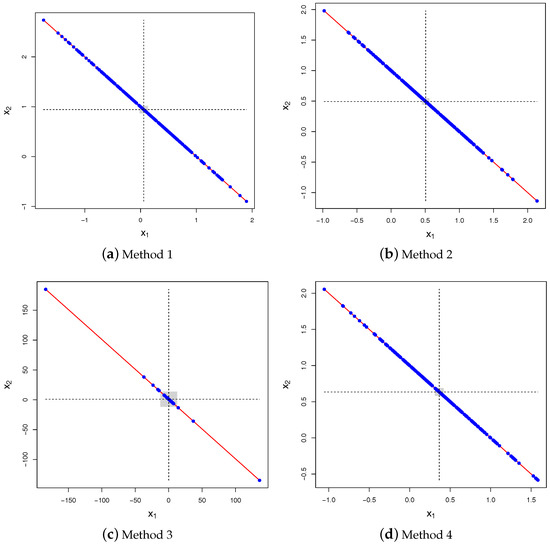
Figure 1. Scatter plot of 250 samples $(x_1,x_2)$ drawn for the four methods with $n=2$, $w_1^2=0.4$, $w_2^2=0.6$ and $c=1$. Method 4 yields the correct answer. The vertical and horizontal dashed lines show the empirical means of $x_1$ and $x_2$ for that specific run, respectively. The diagonal (red) solid line is $x_2=c-x_1$. The horizontal and vertical widths of the gray rectangles show the confidence intervals (${\widehat{\mu }}_{x_i}\pm 1.96\times {\widehat{\sigma }}_{x_i}$) for both $X_1$ and $X_2$ based on 100 runs of 250 pairs each.

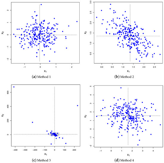
Figure 2. Scatter plot of 250 samples $(x_1,x_2)$ drawn for the four methods with $n=3$, $w_1^2=w_2^2=0.4$, $w_3^2=0.2$ and $c=4$. Method 4 yields the correct answer. Only the first two components of the vector $(x_1,x_2,x_3)$ are shown to enhance readability; the third component is set to $x_3=c-(x_1+x_2)$. The vertical and horizontal dashed lines show the empirical means of $x_1$ and $x_2$ for that specific run, respectively. The horizontal and vertical widths of the gray rectangles show the confidence intervals (${\widehat{\mu }}_{x_i}\pm 1.96\times {\widehat{\sigma }}_{x_i}$) for both $X_1$ and $X_2$ based on 100 runs of 250 pairs each.

4. Sampling Algorithms

From the above result, it is easy to design sampling algorithms. We first derive an algorithm to sample a multivariate Normal distribution under a weighted sum constraint according to the density derived above (Algorithm 1). Next, we show that one can also easily extend this algorithm to sample the multivariate Normal distribution under an upperbound constraint on the weighted sum (Algorithm 2).

Algorithm 1. Sampling of $\mathbf{Z}$ given ${\mathbf{w}}^{\prime }\mathbf{Z}=c$.

1. From the vector of weights $\mathbf{w}$ and the constraint c, compute the $(n-1)$-dimensional mean vector $\mathit{\mu }(c,\mathbf{w})$ and symmetric matrix $\mathsf{\Sigma }\left(\mathbf{w}\right)$ from (2) and (3);

2. Compute the eigen decomposition of the covariance matrix $\mathsf{\Sigma }\left(\mathbf{w}\right)=\mathbf{V}\mathsf{\Lambda }{\mathbf{V}}^{\prime }$;

3. Sample $(n-1)$ i.i.d. standard Normal variates $\tilde{\mathbf{z}}={({\tilde{z}}_1,\dots ,{\tilde{z}}_{n-1})}^{\prime }$;

4. Transform these variates using the mean vector and covariance matrix

$\begin{array}{c}\tilde{\mathbf{x}}\leftarrow \mathit{\mu }(c,\mathbf{w})+\mathbf{V}\sqrt{\mathsf{\Lambda }}\tilde{\mathbf{z}};\end{array}$

5. Enlarge the $(n-1)$-dimensional vector $\tilde{\mathbf{x}}$ with the n-th component to get $\mathbf{x}$,

$\begin{array}{c}\mathbf{x}\leftarrow {\left({\tilde{\mathbf{x}}}^{\prime },c-{\sum }_{i=1}^{n-1}{\tilde{x}}_i\right)}^{\prime };\end{array}$

6. Return $\mathbf{Z}$ where $z_i\leftarrow x_i/w_i$ for $i\in \{1,2,\dots ,n\}$.

The above algorithm can be extended to sample an n-th dimensional vector $\mathbf{Z}$ given ${\mathbf{w}}^{\prime }\mathbf{Z}\le c$. To that end, it suffices to first draw a sample from the conditional distribution of ${\mathbf{w}}^{\prime }\mathbf{Z}$. Clearly, ${\mathbf{w}}^{\prime }\mathbf{Z}\sim \mathcal{N}(0,\parallel \mathbf{w}\parallel )$ so that

$$F_{{\mathbf{w}}^{\prime }\mathbf{Z};c}\left(x\right):=\mathbb{P}({\mathbf{w}}^{\prime }\mathbf{Z}\le x|{\mathbf{w}}^{\prime }\mathbf{Z}\le c)=\left\{\begin{array}{cc}\frac{\mathsf{\Phi }\left(\frac{x}{\parallel \mathbf{w}\parallel }\right)}{\mathsf{\Phi }\left(\frac{c}{\parallel \mathbf{w}\parallel }\right),}\hfill & \mathrm{if}x<c,\hfill \\ 1,\hfill & \mathrm{otherwise}.\hfill \end{array}\right.$$

From the inverse transform, the random variable

$$Y:=F_{{\mathbf{w}}^{\prime }\mathbf{Z};c}^{-1}\left(U\right)$$

has cumulative distribution function $F_{{\mathbf{w}}^{\prime }\mathbf{Z};c}$ whenever U is a Uniform-$[0,1]$ random variable. This leads to the following sampling procedure.

Algorithm 2. Sampling of $\mathbf{Z}$ given ${\mathbf{w}}^{\prime }\mathbf{Z}\le c$.

1. Draw a sample u from a Uniform-$[0,1]$ distribution;

2. Draw a sample $\tilde{c}$ from the conditional law of ${\mathbf{w}}^{\prime }\mathbf{Z}$ given ${\mathbf{w}}^{\prime }\mathbf{Z}\le c$:

$\begin{array}{c}\tilde{c}\leftarrow \parallel \mathbf{w}\parallel {\mathsf{\Phi }}^{-1}\left(u\mathsf{\Phi }\left(\frac{c}{\parallel \mathbf{w}\parallel }\right)\right);\end{array}$

3. Apply Algorithm 1 using $\tilde{c}$ as constraint (i.e., $c\leftarrow \tilde{c}$);

4. Return $\mathbf{Z}$.

Observe that it is very easy to adjust Algorithm 2 to deal with the alternative constraint ${\mathbf{w}}^{\prime }\mathbf{Z}\ge c$. To that end, it suffices to replace $u\mathsf{\Phi }\left(\frac{c}{\parallel \mathbf{w}\parallel }\right)$ by $(1-u)+u\mathsf{\Phi }\left(\frac{c}{\parallel \mathbf{w}\parallel }\right)$.

5. Applications

In this section, we provide two applications that are kept simple on purpose for the sake of illustration.

5.1. Conditional Portfolio Distribution

The application consists of computing the distribution of a portfolio conditional upon the fact that one stock reaches an extreme level, i.e., $S=q_{\alpha }\left(S\right)$ where $q_{\alpha }\left(X\right)$ is the $\alpha$-quantile of the random variable X. We consider K stocks with Normal dollar-returns $S_i\sim \mathcal{N}(m_i,{\sigma }_i^2)$ and note J the dollar-return of a portfolio composed of these stocks with weigths $\pi ={({\pi }_1,{\pi }_2,\dots ,{\pi }_K)}^{\prime }$. We postulate the following n-factor dependence structure:

$$S_i=m_i+{\sigma }_i\left(\sum _{j=1}^n{W}_{i,j}{Z}_j+W_{i,n+1}{ϵ}_i\right),\sqrt{\sum _{j=1}^{n+1}{W}_{i,j}^2}=1,i\in \{1,2,\dots ,K\},$$

where $\mathbf{W}$ is the K-by-$(n+1)$ matrix of loadings, $\mathbf{Z}$ is the vector of n i.i.d. systematic standard Normal risk factors and the ${ϵ}_i$s, $i\in \{1,2,\dots ,K\}$ are the i.i.d. idiosynchratic standard Normal risk factors, independent from the $Z_j$s. Hence,

$$J\sim \sum _{i=1}^K{\pi }_i\left(m_i+{\sigma }_i\left(\sum _{j=1}^n{W}_{i,j}{Z}_j+W_{i,n+1}{ϵ}_i\right)\right).$$

Set $\mathbf{D}=diag({\sigma }_1,\dots ,{\sigma }_K)$, $\mathbf{m}={(m_1,\dots ,m_K)}^{\prime }$ and $\mathbf{M}$ the K-by-n matrix made of the first n columns of $\mathbf{W}$. The portfolio return satisfies $J\sim \mathcal{N}(\tilde{\mu },{\tilde{\sigma }}^2)$ with

$$\begin{array}{ccc}\hfill \tilde{\mu }& =& \sum _{i=1}^K{\pi }_i{m}_i={\mathit{\pi }}^{\prime }\mathbf{m},\hfill \\ \hfill {\tilde{\sigma }}^2& =& \sum _{j=1}^n{\left(\sum _{i=1}^K{\pi }_i{\sigma }_i{W}_{i,j}\right)}^2+\sum _{i=1}^K{\left({\pi }_i{\sigma }_i{W}_{i,n+1}\right)}^2={\mathit{\pi }}^{\prime }\mathbf{D}{\mathbf{MM}}^{\prime }\mathbf{D}\mathit{\pi }+\sum _{i=1}^K{\left({\pi }_i{\sigma }_i{W}_{i,n+1}\right)}^2,\hfill \end{array}$$

where the first term in the right-hand side of ${\tilde{\sigma }}^2$ is the contribution of the n systematic factors and the second results from the K independent idiosynchratic components.

Let us now compute the conditional distribution of the portfolio given that $S_1$ is equal to its percentile $\alpha$, i.e., when

$$S_1=m_1+{\sigma }_1{\mathsf{\Phi }}^{-1}\left(\alpha \right).$$

Noting $c={\mathsf{\Phi }}^{-1}\left(\alpha \right)$, we conclude that

$$\sum _{j=1}^n{W}_{1,j}{Z}_j+W_{1,n+1}{ϵ}_1=c.$$

(9)

Applying the above result with $\mathbf{w}={\mathbf{w}}_1={(W_{1,1},\dots ,W_{1,n+1})}^{\prime }$, the density of the random vector $(W_{1,j}{Z}_1,\dots ,W_{1,n}{Z}_n,W_{1,n+1}{ϵ}_1)$ conditional upon (9) is jointly Normal with mean vector $\mathit{\mu }$ and covariance matrix $\mathsf{\Sigma }$ given by

$$\begin{array}{ccc}\hfill {\mu }_i& :=& {\mu }_i(c,{\mathbf{w}}_1)=c{W}_{1,i}^2,\hfill \\ \hfill {\mathsf{\Sigma }}_{i,j}& :=& {\mathsf{\Sigma }}_{i,j}\left({\mathbf{w}}_1\right)=W_{1,i}^2\left({\delta }_{ij}\left(1-W_{1,i}^2\right)+({\delta }_{ij}-1)W_{1,j}^2\right)=W_{1,i}^2\left({\delta }_{ij}-W_{1,j}^2\right),\hfill \end{array}$$

where $i,j$ in $\{1,2,\dots ,n+1\}$. In order to find the joint distribution of $\mathbf{Z}$, we need to correct for the scaling coefficients and disregard ${ϵ}_1$. Correcting for the scaling coefficients simply requires rescaling the entries of the mean vector and covariance matrix by $1/W_{1,i}$ and $1/\left(W_{1,i}{W}_{1,j}\right)$, respectively. The conditional distribution of $\mathbf{Z}$ is a n-dimensional Normal with mean vector and covariance matrix found by taking the first n entries of the above mean vector and the n-by-n upper-left of the covariance matrix. This leads to

$${\mu }_i=c{W}_{1,i},{\mathsf{\Sigma }}_{i,j}=\frac{W_{1,i}}{W_{1,j}}\left({\delta }_{ij}-W_{1,j}^2\right),i,j\in \{1,2,\dots ,n\}.$$

The eigen decomposition of the covariance matrix is noted $\mathsf{\Sigma }=\mathbf{V}\mathsf{\Lambda }{\mathbf{V}}^{\prime }$, so that $\mathbf{Z}\sim \mu +\mathbf{V}\sqrt{\mathsf{\Lambda }}\tilde{\mathbf{Z}},$ where $\tilde{\mathbf{Z}}$ is a n-variate vector of independent standard Normal variables.

Let us note ${\mathit{\pi }}^j$ the vector $\mathit{\pi }$ whose j-th entry is set to 0, i.e., ${\mathit{\pi }}^j=\mathit{\pi }-{\pi }_j{\mathbf{e}}_j$ where ${\mathbf{e}}_j$ is the j-th basis vector. Letting $\widehat{\mathbf{Z}}$ be a standard Normal random variable independent from $\tilde{\mathbf{Z}}$,

$$\begin{array}{ccc}\hfill J& \sim & {\mathit{\pi }}^{\prime }\mathbf{m}+{\pi }_1{\sigma }_{1}c+{{\mathit{\pi }}^1}^{\prime }\mathbf{DM}\mathit{\mu }+{{\mathit{\pi }}^1}^{\prime }\mathbf{DMV}\sqrt{\mathsf{\Lambda }}\tilde{\mathbf{Z}}+\sqrt{\sum _{i=2}^K{\left({\pi }_i{\sigma }_i{W}_{i,n+1}\right)}^2}\widehat{\mathbf{Z}}\hfill \end{array}$$

so that $J\sim \mathcal{N}\left(\tilde{\mu },{\tilde{\sigma }}^2\right)$ where

$$\begin{array}{ccc}\hfill \tilde{\mu }& =& {\mathit{\pi }}^{\prime }\mathbf{m}+{\pi }_1{\sigma }_{1}c+{{\mathit{\pi }}^1}^{\prime }\mathbf{DM}\mathit{\mu },\hfill \\ \hfill {\tilde{\sigma }}^2& =& {{\mathit{\pi }}^1}^{\prime }\mathbf{DM}\mathsf{\Sigma }{\mathbf{M}}^{\prime }\mathbf{D}{\mathit{\pi }}^1+\sum _{i=2}^K{\left({\pi }_i{\sigma }_i{W}_{i,n+1}\right)}^2.\hfill \end{array}$$

5.2. Expected Shortfall of a Defaultable Portfolio

The next example consists of approximating the Conditional Value-at-Risk (a.k.a. Expected Shortfall) associated with the portfolio of m defaultable assets in a multi-factor model. The total loss L on such a portfolio up to the time horizon T is the sum of the individual losses $L={\sum }_{i=1}^m{L}_i$, where the contribution of the loss of the i-th asset is of the form $L_i=w_i{1}_{\{{\tau }_i\le T\}}$, where $w_i$ is the weight of the asset in the portfolio and ${\tau }_i$ is the default time of the i-th obligor. Whereas the expected loss is independent from the possible correlation across defaults, it is a key driver of the Value-at-Risk, and hence of the economic and regulatory capital. Most credit risk models introduce such dependency by relying on latent variables, like $1_{\{{\tau }_i\le T\}}\iff 1_{\{{\xi }_i\le F^{-1}\left({\pi }_i\right)\}}$, where the ${\xi }_i$s are correlated random variables with cumulative distribution function F and ${\pi }_i$ is the marginal probability that ${\tau }_i\le T$ under the chosen measure. The most popular choice (although debatable) is to rely on multi-factor Gaussian models, i.e., to consider ${\xi }_i={\mathbf{w}}_i^{\prime }\mathbf{Z}+\sqrt{1-\parallel {\mathbf{w}}_i{\parallel }^2}{ϵ}_i$, where ${\mathbf{w}}_i$ is a n-dimensional vector of weights with norm smaller than 1, $\mathbf{Z}$ is the vector of n i.i.d. standard Normal systematic factors and the ${ϵ}_i$ are i.i.d. standard Normal random variables independent from the $Z_j$s representing the idiosynchratic risks. Computing the Expected Shortfall in a multi-factor framework is very time-consuming as there is no closed-form solution and many simulations are required. A possible alternative to the plain Monte Carlo estimator is to rely on the ASRF${}^{*}$ model of Pykhtin, which can be seen as the single-factor model that “best” approximates the multi-factor model in the left tail, in some sense (see Pykhtin (2004) for details). The ASRF${}^{*}$ model thus deals with a loss variable $L^{*}$ relying on a single factor Y, but such that $q_{\alpha }\left(L^{*}\right)\approx q_{\alpha }\left(L\right),$ where L is the loss variable in the multi-factor model. By the law of large numbers, the idiosynchratic risks are diversified away for m large enough, so that conditional upon $Y=x$, the portfolio loss in the ASRF${}^{*}$ model converges almost surely, as $m\to \infty$, to $L^{*}\left(x\right)$ with $L^{*}\left(Y\right):=\mathbb{E}\left[L^{*}\right|Y]$. Moreover, $L^{*}\left(x\right)$ is a monotonic and decreasing function of x. Consequently, the Value-at-Risk of the ASRF${}^{*}$ model satisfies $q_{\alpha }\left(L^{*}\right)\approx L^{*}\left({\mathsf{\Phi }}^{-1}(1-\alpha )\right)$ for m large enough. The asymptotic analytical expression $L^{*}\left({\mathsf{\Phi }}^{-1}(1-\alpha )\right)$ is known as the large pool approximation (see e.g., Gordy (2003)). In the derivation of the ASRF${}^{*}$ analytical formula, Pykhtin implicitly models Y as a linear combination of the factors $Z_j$ appearing in the multi-factor model, i.e., $Y={\mathbf{b}}^{\prime }\mathbf{Z}$ s.t. $\parallel \mathbf{b}\parallel =1$. One can thus draw samples for the $Z_j$s by using Algorithm 2 as follows: (i) draw a value for the standard Normal factor Y conditional upon $Y\le {\mathsf{\Phi }}^{-1}(1-\alpha )$, i.e., set $Y={\mathsf{\Phi }}^{-1}\left(U(1-\alpha )\right)$ with U a Uniform-$[0,1]$ random variable so that $L^{*}\left(Y\right)\ge L^{*}\left({\mathsf{\Phi }}^{-1}(1-\alpha )\right)$, and then (ii) sample $\mathbf{Z}$ conditional upon ${\mathbf{b}}^{\prime }\mathbf{Z}=Y$ from the joint density derived in the paper. Therefore, we use $L^{*}\left(Y\right)\ge L^{*}\left({\mathsf{\Phi }}^{-1}(1-\alpha )\right)$ as a proxy for the condition $L\ge q_{\alpha }\left(L\right)$ involved in the expected shortfall definition (observe that both L and $L^{*}$ depend on the same random vector $\mathbf{Z}$), but use the actual (multi-factor) loss to estimate the expected loss under this condition. In other words, we effectively compute $\widehat{\mathbb{E}}\left[L\right|L^{*}\left({\mathbf{b}}^{\prime }\mathbf{Z}\right)\ge L^{*}\left({\mathsf{\Phi }}^{-1}(1-\alpha )\right)]$ as a proxy of the genuine Expected Shortfall, defined as $\mathbb{E}\left[L\right|L\ge q_{\alpha }\left(L\right)]$, leading to a drastic reduction of the computational cost.

6. Conclusions

Many practical applications in the area of risk management deal with factor models, and often these factors are taken to be Gaussian. In various cases, it can be interesting to analyse the picture under some constraints on the weighted sum of these factors. This might be the case for instance when it comes to perform scenario analyses in adverse circumstances, to compute conditional risk measures or to speed up simulations (in the same vein as importance sampling). In this paper, we derive the density of a n-dimensional Normal vector with independent components subject to the constraint that the weighted sum takes a given value. It is proven to be a $(n-1)$-multivariate Normal whose mean vector and covariance matrix can be computed in closed-form by relying on the specific structure of the (inverse) covariance matrix. This result naturally leads to various sampling algorithms, e.g., to draw samples with weighted sum being equal to, below or above a given threshold. Interestingly, the proposed scheme is shown to differ from various “standard rescaling” procedures applied to independent samples. Indeed, the latter fail to comply with the actual conditional distribution found, both in terms of expectation and variance.

References

- Andersen, Leif B. G., and Jakob Sidenius. 2004. Extensions to the Gaussian copula: Random recovery and random factor loadings. Journal of Credit Risk 1: 29–70. [Google Scholar] [CrossRef]
- Cedilnik, Anton, Katarina Kosmelj, and Andrej Blejec. 2004. The distribution of the ratio of jointly Normal variables. Metodološki Zvezk 1: 99–108. [Google Scholar]
- Fieller, Edgar C. 1932. The distribution of the index in a normal bivariate population. Biometrika 23: 428–40. [Google Scholar] [CrossRef]
- Gentle, James E. 2007. Matrix Algebra: Theory, Computations, and Applications in Statistics. Berlin: Springer. [Google Scholar]
- Glasserman, Paul. 2010. Monte Carlo Methods in Financial Engineering. Berlin: Springer. [Google Scholar]
- Gordy, Michael B. 2003. A risk-factor model foundation for ratings-based bank capital rules. Journal of Financial Intermediation 12: 199–232. [Google Scholar] [CrossRef]
- Hull, John, and Alan White. 2004. Valuation of a CDO and an nth-to-default CDS without Monte Carlo simulation. Journal of Derivatives 12: 8–23. [Google Scholar] [CrossRef]
- Laurent, Jean-Paul, Michael Sestier, and Stéphane Thomas. 2016. Trading book and credit risk: how fundamental is the Basel review? Journal of Banking and Finance 73: 211–23. [Google Scholar] [CrossRef]
- Li, David X. 2016. On Default Correlation: A Copula Function Approach. Technical Report. Amsterdam: Elsevier. [Google Scholar]
- Meyer, Daniel W. 2018. (un)conditional sample generation based on distribution element trees. Journal of Computational and Graphical Statistics. [Google Scholar] [CrossRef]
- Pham, Dinh Tuan. 2000. Stochastic methods for sequential data assimilation in strongly nonlinear systems. Monthly Weather Review 129: 1194–207. [Google Scholar] [CrossRef]
- Pykhtin, Michael. 2004. Multifactor adjustment. Risk Magazine 17: 85–90. [Google Scholar]
- Rubinstein, Reuven Y., and Dirk Kroese. 2017. Simulation and the Monte Carlo Method. Hoboken: Wiley. [Google Scholar]
- Vasicek, Oldrich A. 1991. Limiting loan loss probability distribution. Finance, Economics and Mathematics. [Google Scholar] [CrossRef]
- Vrins, Frederic D. 2009. Double-t copula pricing of structured credit products—Practical aspects of a trustworthy implementation. Journal of Credit Risk 5: 91–109. [Google Scholar] [CrossRef]
© 2018 by the author. Licensee MDPI, Basel, Switzerland. This article is an open access article distributed under the terms and conditions of the Creative Commons Attribution (CC BY) license (http://creativecommons.org/licenses/by/4.0/).