Deep Arbitrage-Free Learning in a Generalized HJM Framework via Arbitrage-Regularization

Abstract

A regularization approach to model selection, within a generalized HJM framework, is introduced, which learns the closest arbitrage-free model to a prespecified factor model. This optimization problem is represented as the limit of a one-parameter family of computationally tractable penalized model selection tasks. General theoretical results are derived and then specialized to affine term-structure models where new types of arbitrage-free machine learning models for the forward-rate curve are estimated numerically and compared to classical short-rate and the dynamic Nelson-Siegel factor models.

1. Introduction

The compatibility of penalized regularization with machine learning approaches allows for the successful treatment of various challenges in learning theory such as variable selection (see Tibshirani (1996)) and dimension reduction (see Zou et al. (2006)). The objective of many machine learning models used in mathematical finance is to predict asset prices by learning functions depending on stochastic inputs. In general, there is no guarantee that these stochastic factor models are consistent with no-arbitrage conditions. This paper introduces a novel penalized regularization approach to address this modelling difficulty in a manner consistent with financial theory. The incorporation of an arbitrage-penalty term allows various machine learning methods to be directly and coherently integrated into mathematical finance applications. We focus on regression-type model selection tasks in this article. However, the arbitrage-penalty can also be applied to other types of machine learning algorithms with financial applications.

To motivate our approach we first consider informally, similar to (Björk 2009, Chapter 10), the following simple situation that will later be made more precise. Let $(\Omega ,\mathcal{F},{\left({\mathcal{F}}_t\right)}_{t\ge 0},\mathbb{P})$ be a filtered probability space satisfying the usual conditions. Let ${\left(X_t\right)}_{t\ge 0}$ be an ${\mathcal{F}}_t$-adapted real-valued stochastic process with continuous paths representing the price of a financial asset. Let r be the constant risk-free interest rate and assume a fixed time interval $[0,T]$. Existence of a martingale measure $\mathbb{Q}$ equivalent to the underlying real-world measure $\mathbb{P}$ implies absence of arbitrage. The price at time $t\in [0,T]$ of a derivative security with integrable payoff $f\left(X_T\right)$ at time T is given by the risk-neutral pricing formula

$${\mathbb{E}}_{\mathbb{Q}}\left[e^{-r(T-t)}f\left(X_T\right)|{\mathcal{F}}_t\right].$$

(1)

With $L_t=\frac{d\mathbb{Q}}{d\mathbb{P}}{|}_{{\mathcal{F}}_t}$ we may express Equation (1) under the real-world probability measure $\mathbb{P}$ as

$${\mathbb{E}}_{\mathbb{P}}\left[e^{-r(T-t)}\frac{L_T}{L_t}f\left(X_T\right)|{\mathcal{F}}_t\right].$$

(2)

Equivalently, the price given by Equation (2) can be expressed under $\mathbb{P}$ by defining the state-price density process $Z_t=e^{-rt}{L}_t$. If $\mathbb{Q}$ is the minimal martingale measure of Schweizer (1995) then the transformation

$$f\left(X_t\right)\mapsto Z_{t}f\left(X_t\right)$$

(3)

can be interpreted as finding the process closest to ${\left(f\left(X_t\right)\right)}_{t\ge 0}$ which is a (local) martingale under $\mathbb{P}$. The purpose of this paper is to find an analogue of the transformation (3) in this setting when $X_t$ is described by a stochastic factor model, as is the case with most machine learning approaches to mathematical finance. For example, $X_t$ may be described by a deep neural network with stochastic inputs.

The above-ignored well-known results regarding the uniqueness of $\mathbb{Q}$ (see Schweizer (1995)) and other important generalizations of the martingale approach to arbitrage theory. In particular, the more general setting for the fundamental theorem of asset pricing of Delbaen and Schachermayer (1998) implies that if “arbitrage”, in the sense of no-free lunch with vanishing risk, exists then the transformation (3) is undefined. However, many machine learning approaches to mathematical finance may admit arbitrage so it is necessary to consider the general case. The arbitrage-regularization framework introduced in this paper integrates machine learning methodologies with the general martingale approach to arbitrage theory.

We consider a general framework for learning the arbitrage-free factor model that is most similar to a factor model within a prespecified class of alternative factor models. This search is optimized by minimizing a loss-function measuring the distance of the alternative model to the original factor model with the additional constraint that the market described by the alternative model is a local martingale under a reference probability measure.

The main theoretical results rely on asymptotics for the arbitrage-regularization penalty for selecting the optimal arbitrage-free model from a class of stochastic factor models. Relaxation of the asymptotic results necessary for practical implementation are presented. Throughout this paper, the bond market will serve as the primary example of our methods since no-arbitrage conditions for factor models are well understood, see Filipović (2001) and the references therein. Numerical results applying the arbitrage-regularization methodology are implemented using real data.

The remainder of this paper is organized as follows. Section 2 states the arbitrage-regularization problem and presents an overview of relevant background on bond markets. Section 3 develops the arbitrage-penalty and establishes the main asymptotic optimality results. Non-asymptotic relaxations of these results are also considered and linked with transaction costs. Section 4 specializes the general results to bond markets and where a simplified expression for the arbitrage-penalty is obtained. Numerical implementations of the results are considered and the arbitrage-regularization methodology is used to generate new machine learning-based models consistent with no free lunch with vanishing risk (NFLVR) and the results are compared with classical term-structure models as benchmarks. Section 5 concludes and Appendix A contains supplementary material primarily required for the proofs, such as functional Itô calculus and $\Gamma$-convergence results. Proofs of the main theorems of the paper are included in Appendix B.

2. The Arbitrage-Regularization Problem

For the remainder of the paper all stochastic processes described in this paper are defined on a common stochastic basis $\left(\Omega ,\mathcal{F},{\left({\mathcal{F}}_t\right)}_{t\ge 0},\mathbb{P}\right)$. Let ${\mathbb{P}}^{★}$ be a probability measure equivalent to the reference probability measure $\mathbb{P}$ and ${\left(r_t\right)}_{t\ge 0}$ denotes the risk-free rate in effect at time $t\ge 0$. Assume that there exists an asset whose price process, denoted by ${\left(N_t\right)}_{t\ge 0}$, is a strictly positive ${\mathbb{P}}^{★}$-martingale which serves as numéraire. Unless otherwise specified all the processes in this paper will be described under the martingale-measure for ${\left(N_t\right)}_{t\ge 0}$, denoted ${\mathbb{P}}_N$ is defined by

$$\frac{d{\mathbb{P}}_N^{★}}{d{\mathbb{P}}^{★}}=exp\left({\int }_0^T-r_{s}ds\right)\frac{N_T}{N_0}.$$

The choice of the numéraire can be used to encode or remove any trend from the price processes being modelled. Price processes which are local martingales under ${\mathbb{P}}_N^{★}$ or ${\mathbb{P}}^{★}$ are usually only semi-martingales under the objective measure $\mathbb{P}$. Further details on numéraires can be found in Shreve (2004).

We consider a large financial market ${\left(X_t\left(u\right)\right)}_{t\ge 0,u\in \mathcal{U}}$, indexed by a non-empty Borel subset $\mathcal{U}\subseteq {\mathbb{R}}^D$, were D is a positive integer. For example, ${\left(X_t\left(u\right)\right)}_{t\ge 0,u\in \mathcal{U}}$ may be used to represent a bond market where, using the parameterization of Musiela and Rutkowski (1997), $\mathcal{U}=[0,\infty )$ represents the collection of all possible maturities and $X_t\left(u\right)$ represents the time t price of a zero-coupon bond with maturity u.

For each $u\in \mathcal{U}$, the process ${\left(X_t\left(u\right)\right)}_{t\ge 0}$ will be driven by a latent, possibly infinite-dimensional, factor process. In the case of the bond market, this latent process will be the forward-rate curve. Write

$$\begin{array}{cc}\hfill X_t\left(u\right)\triangleq & S_t\left({\varphi }_t^u,{\left[\left[{\varphi }^u\right]\right]}_t;u\right)\hfill \end{array}$$

(4)

where ${\varphi }_t^u\triangleq \varphi (t,{\beta }_t,u)$, ${\left\{S_t(·,·;u)\right\}}_{u\in \mathcal{U}}$ is a family of path-dependent functionals encoding the latent process into the asset price $X_t\left(u\right)$, ${\varphi }_t^u$ is the factor model for the latent process, and ${\beta }_t$ are the ${\mathbb{R}}^d$-valued stochastic factors driving the latent process. Following Fournie (2010), $S_t$ will be allowed to depend on the local quadratic-variation of the factor process $\varphi (t,{\beta }_t,u)$, denoted by ${\left[\left[{\varphi }^u\right]\right]}_t$ and defined by

$${\left[\varphi (·,{\beta }_{·},u)\right]}_t={\int }_0^t{\left[\left[{\varphi }^u\right]\right]}_{s}ds,$$

where ${\left[\varphi (·,{\beta }_{·},u)\right]}_t$ denotes the usual quadratic-variation of the factor process ${\left[\varphi (·,{\beta }_{·},u)\right]}_t$. It is instructive to note that the local quadratic-variation ${\left[\left[{\varphi }^u\right]\right]}_t$ is well-defined due to Assumption 1, imposed later.

In the case of the bond market, $S_t$ will be the map taking a forward-rate curve, such as ${\left(\varphi (t,{\beta }_t,u)\right)}_{u\in \mathcal{U}}$, to the time t price of a zero-coupon bond with maturity u, as defined by

$$S_t\left({\varphi }_t^u,{\left[\left[{\varphi }^u\right]\right]}_t;u\right)\triangleq exp\left(-{\int }_t^u\varphi (t,{\beta }_t,v)dv\right).$$

(5)

It will often be convenient to use the reparameterization of Musiela and Rutkowski (1997) and rewrite (6) as

$$S_t\left({\varphi }_t^u,{\left[\left[{\varphi }^u\right]\right]}_t;u\right)\triangleq exp\left(-{\int }_0^{u-t}\varphi (t,{\beta }_t,\tau )d\tau \right).$$

(6)

where $\tau \triangleq u-s$, for $0\le t\le s\le u$, and represents the time to maturity of the bond.

In general, $S_t$ will be allowed to depend on the path of $\varphi (t,{\beta }_t,u)$. Thus, $S_t$ will be a path-dependent functional of regularity ${\mathbb{C}}_b^{1,2}$ in the sense of Fournie (2010) as discussed in Appendix A.2. However, as in the bond market, if $S_t$ depends only on the current value of $\varphi (t,{\beta }_t,u)$ then the requirement that $S_t$ be of class ${\mathbb{C}}_b^{1,2}$, in the sense of Fournie (2010), is equivalent to it being of regularity $C^{1,2}(I\times {\mathbb{R}}^d)$ in the classical sense; where $I\triangleq [0,\infty )$. Therefore, the classical Itô-calculus would apply to $S_t$.

Analogously to Björk and Christensen (1999), the factor model $\phi$ for the latent process will always be assumed to be suitably integrable and suitably differentiable. Specifically, $\phi$ will belong to a Banach subspace $\mathcal{X}$ of $L_{\nu \otimes \mu }^p\left(I\times {\mathbb{R}}^d\times \mathcal{U}\right)$ which can be continuously embedded within the Fréchet space $C^{1,2,2}(I\times {\mathbb{R}}^d\times \mathcal{U})$; where $\nu$ is a Borel probability measure supported on I, $\mu$ is a Borel probability measure supported on ${\mathbb{R}}^d\times \mathcal{U}$, and both $\nu$ and $\mu$ are equivalent to the corresponding Lebesgue measures restricted to their supports. Here, $1\le p<\infty$ is kept fixed.

An example from the bond modelling literature is the Nelson-Siegel model (see Nelson and Siegel (1987) and Diebold and Rudebusch (2013)), which expresses the forward-rate curve as a function of its level, slope, and curvature through the factor model. The Nelson-Siegel family is part of a larger class of affine term-structure models, in which, at any given time, the forward-rate curve is described in terms of a set of market factors as

$$\begin{array}{c}\hfill \phi (t,\beta ,u)\triangleq {\phi }_0(u-t)+\sum _{i=1}^d{\beta }^i{\phi }_i(u-t),\end{array}$$

(7)

where d is a positive integer and ${\phi }_i\in C^2\left(\mathcal{U}\right)$ and ${\phi }_0$ is a forward-rate curve typically calibrated to the data available at time $t=0$. Note that the forward-rate curves in (7) are parameterized according to the change of variables in (6), however, since $\mathcal{U}$ represents all times to maturities these are indeed traded assets. However, as shown in Filipović (2001), the Nelson-Siegel model is typically not arbitrage-free therefore we would like to learn the closest arbitrage-free factor model, driven by the same stochastic factors. Therefore, given a non-empty and unbounded hypothesis class $\mathcal{H}\subseteq \mathcal{X}$ of plausible alternative models, we optimize

$$\begin{array}{cc}\hfill & {\mathrm{argmin}}_{[\varphi \in \mathcal{H}]}\ell \left(\phi -\varphi \right)\hfill \\ \hfill & \mathrm{subject} \mathrm{to}:S_t({\varphi }_t^u,{\left[\left[{\varphi }^u\right]\right]}_t;u)\mathrm{is} \mathrm{a} {}_N^{★}-\mathrm{local} \mathrm{martingale} \mathrm{for} \mathrm{all} u\in \mathcal{U};\hfill \end{array}$$

(8)

where $\mathcal{H}$ is required to contain the (naive) factor model $\phi$ and $\ell :\mathcal{X}\to [0,\infty )$ is continuous and coercive loss function. For example, ℓ may be taken to be the norm on $\mathcal{X}$. Geometrically, (8) describes a projection of $\phi$ onto the (possibly non-convex) subset of $\mathcal{H}$ of factor models making each $S_t({\varphi }_t^u,{\left[\left[{\varphi }^u\right]\right]}_t;u)$ into a ${\mathbb{P}}_N^{★}$-local martingale for every $u\in \mathcal{U}$. The requirement that $\mathcal{H}$ contains the (naive) factor model $\phi$ is for consistency, in order to ensure that for any arbitrage-free factor model $\phi$ the solution to problem (8) is itself.

In general, the problem described by (8) may be challenging to implement as projections onto non-convex sets are intractable. In analogy with regularization literature, such as Hastie et al. (2015), instead we consider the following relaxation of problem (8) which is more amenable to numerical implementation

$${\mathrm{argmin}}_{[\varphi \in \mathcal{H}]}\ell \left(\phi -\varphi \right)+{\mathrm{AF}}^{\lambda }\left(\varphi \right);$$

(9)

where ${\left\{{\mathrm{AF}}^{\lambda }\right\}}_{2\le \lambda <\infty }$ is a family of functions from $\mathcal{H}$ to $[0,\infty ]$ taking value 0 if each

$S_t({\varphi }_t^u,{\left[\left[{\varphi }^u\right]\right]}_t;u)$ is a ${\mathbb{P}}_N^{★}$-local martingale simultaneously for every value of u and $\lambda$ is a meta-parameter determining the amount of emphasis placed on the penalizing factor models which fail to meet this requirement. Problem (9) is called the arbitrage-regularization problem.

At the moment, there are only two available lines of research which are comparable to the arbitrage-regularization problem. Results of the first kind, such as the arbitrage-free Nelson-Siegel model of Christensen et al. (2011a), provide closed-form case-by-case arbitrage-free variants of specific model only if they coincide with specific arbitrage-free HJM type factor models, such as those studied by Björk and Christensen (1999). However, the reliance on analytic methods typically limit this type of approach to simple or specific models and does not allow for a general or computationally viable solution to the problem. Moreover, arbitrage-free corrections derived in this way are not guaranteed to be optimal in the sense of (8), or approximately optimal in the sense of (9). This will be examined further in the numerics section of this paper.

The use of a penalty to capture no-arbitrage conditions has, to the best of the authors’ knowledge, thus far only been explored numerically by Chen et al. (2019) within the discrete-time portfolio optimization setting. A similar problem has been treated in Chen et al. (2006) for learning the equivalent martingale measure in the multinomial tree setting for stock prices. Our paper provides the first instance of a theoretical result in this direction as well as such a framework that applies to large-financial markets such as bond markets or which applies in the continuous-time setting.

Before presenting the main results we first state necessary assumptions.

Assumption 1.

The following assumptions will be maintained throughout this paper.

(i) 

${\beta }_t$ is an ${\mathbb{R}}^d$-valued diffusion process which is the unique strong solution to

$${\beta }_t={\beta }_0+{\int }_0^t\alpha (s,{\beta }_s)ds+{\int }_0^t\sigma (s,{\beta }_s)d{W}_s,$$

(10)

where ${\beta }_0\in {\mathbb{R}}^d$, $W_t$ is an ${\mathbb{R}}^d$-valued Brownian motion, the components ${\alpha }^i:{\mathbb{R}}^{1+d}\to \mathbb{R}$ are continuous, the components ${\left({\sigma }^{i,j}:{\mathbb{R}}^{1+d}\to {\mathbb{R}}^{d\times d}\right)}_{i,j=1}^d$ are measurable and such that the diffusion matrix

$$\sigma (s,\beta )\sigma {(s,\beta )}^{\top }$$

is a continuous function of β for any fixed $t\ge 0$.

(ii) 

The stochastic differential equation (10) has a unique ${\mathbb{R}}^d$-valued solution for each ${\beta }_0\in {\mathbb{R}}^d$.

(iii) 

For every $u\in \mathcal{U}$, ${\left\{S_t(·,·;u)\right\}}_{t\in [0,\infty )}$ is a non-anticipative functional in ${\mathbb{C}}_b^{1,2}$ verifying the following “predictable-dependence” condition of Fournie (2010):

$$\begin{array}{cc}\hfill S_t(x_t,x_t;u)& =S_t(x_t,x_{t_{-}};u),\hfill \end{array}$$

for all $t\in [0,\infty )$ and all $(x,v)\in D([0,t];{\mathbb{R}}^d)\times D([0,t];S_{+}^d)$, where $S_{+}^d$ is the set of $d\times d$-dimensional positive semi-definite matrices with real-coefficients,

The central problem of the paper will be addressed in full generality before turning to applications in term-structure models, in the next section.

3. Main Results

In this section, we show the asymptotic equivalence of problems (8) and (9) for general asset classes. This requires the construction of the penalty term ${\mathrm{AF}}^{\lambda }$ measuring how far a given factor model is from being a ${\mathbb{P}}_N^{★}$-local martingale. The construction of ${\mathrm{AF}}^{\lambda }$ is made in two steps. First, a drift condition which guarantees that each ${\left\{S_t({\varphi }_t^u,{\left[\left[{\varphi }^u\right]\right]}_t;u)\right\}}_{u\in \mathcal{U}}$ is simultaneously a ${\mathbb{P}}_N^{★}$-local martingale is obtained. This condition generalizes the drift condition of Heath et al. (1992) and provides an analogue to the consistency condition of Filipović and Teichmann (2004). Second, the drift condition is used to produce the penalty term in (9). Subsequently, the optimizers of (9) will be used to asymptotically solve problem (8).

Proposition 1

(Drift Condition). The processes $S_t({\varphi }_t^u,{\left[\left[{\varphi }^u\right]\right]}_t;u)$ are ${\mathbb{P}}_N^{★}$-local-martingales, for each $u\in \mathcal{U}$ simultaneously, if and only if

$$\begin{array}{cc}\hfill -\mathcal{D}{S}_s({\varphi }_s^u,{\left[\left[{\varphi }^u\right]\right]}_s;u)=& \nabla S_s({\varphi }_s^u,{\left[\left[{\varphi }^u\right]\right]}_s;u)\left[\frac{\partial \varphi }{\partial t}(s,{\beta }_s,u)+\sum _{i=1}^d\frac{\partial \varphi }{\partial {\beta }^i}(s,{\beta }_s,u){\alpha }^i(s,{\beta }_s)\right.\hfill \\ \hfill +& \left.\frac{1}{2}\sum _{i,j=1}^d\left(\frac{{\partial }^2\varphi }{\partial {\beta }^i\partial {\beta }^j}(s,{\beta }_s,u)\right){\sigma }^i(s,{\beta }_s){\sigma }^j(s,{\beta }_s)\right]\hfill \\ \hfill +& \frac{1}{2}\left[{\nabla }^2{S}_s({\varphi }_s^u,{\left[\left[{\varphi }^u\right]\right]}_s;u)\right]{\left(\sum _{i=1}^d\frac{\partial \varphi }{\partial {\beta }^i}(s,{\beta }_s,u){\sigma }^i(s,{\beta }_s)\right)}^2.\hfill \end{array}$$

(11)

is satisfied ${\mathbb{P}}_N^{★}$-a.s. for every $t\in [0,\infty )$ and every $u\in \mathcal{U}$, where $\mathcal{D}$ and ∇ respectively denote the horizontal and vertical derivative of Fournie (2010) (see Appendix A.2 Equation (A3)).

The drift condition in Proposition 1 implies that if $\varphi$ is such that the difference of the left and right-hand sides of (11) is equal to 0, ${\mathbb{P}}_N^{★}$-a.s. for all $u\in \mathcal{U}$ then $S_t({\varphi }_t^u,{\left[\left[{\varphi }^u\right]\right]}_t;u)$ is a ${\mathbb{P}}_N^{★}$-local martingale simultaneously for all $u\in \mathcal{U}$. Thus, $S_t({\varphi }_t^u,{\left[\left[{\varphi }^u\right]\right]}_t;u)$ is simultaneously a ${\mathbb{P}}_N^{★}$-local martingale for all $u\in \mathcal{U}$ if for every $u\in \mathcal{U}$ the $[0,\infty )$-valued process ${\underline{\mathsf{\Lambda }}}_t^u\left(\varphi \right)$ is equal to 0 ${\mathbb{P}}_N^{★}$-a.s, where ${\underline{\mathsf{\Lambda }}}_t^u\left(\varphi \right)$ is defined using (11) by

$$\begin{array}{ll}\hfill {\underline{\mathsf{\Lambda }}}_t^u\left(\varphi \right)\triangleq & \left|\mathcal{D}{S}_s({\varphi }_s^u,{\left[\left[{\varphi }^u\right]\right]}_s;u)+\nabla S_s({\varphi }_s^u,{\left[\left[{\varphi }^u\right]\right]}_s;u)\left[\frac{\partial \varphi }{\partial t}(s,{\beta }_s,u)+\sum _{i=1}^d\frac{\partial \varphi }{\partial {\beta }^i}(s,{\beta }_s,u){\alpha }^i(s,{\beta }_s)\right.\right.\hfill \\ \hfill +& \left.\frac{1}{2}\sum _{i,j=1}^d\left(\frac{{\partial }^2\varphi }{\partial {\beta }^i\partial {\beta }^j}(s,{\beta }_s,u)\right){\sigma }^i(s,{\beta }_s){\sigma }^j(s,{\beta }_s)\right]\hfill \\ \hfill +& \left.\frac{1}{2}\left[{\nabla }^2{S}_s({\varphi }_s^u,{\left[\left[{\varphi }^u\right]\right]}_s;u)\right]{\left(\sum _{i=1}^d\frac{\partial \varphi }{\partial {\beta }^i}(s,{\beta }_s,u){\sigma }^i(s,{\beta }_s)\right)}^2\right|,\hfill \end{array}$$

(12)

where ${\varphi }_t^u=\varphi (t,{\beta }_t,u)$. The arbitrage-penalty is defined as follows.

Definition 1

(Arbitrage-Penalty). Let ${\left\{{\left({\mathsf{\Lambda }}_t^u\left(\varphi \right)\right)}_{t\ge 0}\right\}}_{\varphi \in \mathcal{H};u\in \mathcal{U}}$ be a family of ${\mathcal{F}}_t$-adapted $[0,\infty )$-valued stochastic processes for which

$$\begin{array}{cc}\hfill {\mathsf{\Lambda }}_t^u\left(\varphi \right)\left(\omega \right)=0& \iff {\underline{\mathsf{\Lambda }}}_t^u\left(\varphi \right)\left(\omega \right)=0,\hfill \end{array}$$

(13)

holds for all $\varphi \in \mathcal{H}$, $t\in I$, $u\in \mathcal{U}$, and ${\mathbb{P}}_N^{★}$-almost every $\omega \in \Omega$. Then, for every $\lambda \ge 0$, the family ${\left\{{\mathrm{AF}}^{\lambda }\right\}}_{\lambda \ge 0}$ of functions

$$\begin{array}{cc}\hfill & {\mathrm{AF}}^{\lambda }:\mathcal{X}\to [0,\infty ]\hfill \\ \hfill & \varphi \mapsto \lambda \sqrt[\lambda ]{{\int }_{(t,u)\in I\times \mathcal{U}}{\left|{\mathsf{\Lambda }}_t^u\left(\varphi \right)\right|}^{\lambda }d\mu (t,u)}.\hfill \end{array}$$

(14)

is said to define an arbitrage-penalty.

Remark 1.

Whenever $|{\mathsf{\Lambda }}_t^u{\left(\varphi \right)|}^{\lambda }$ fails to be integrable, we make the convention that $\sqrt[\lambda ]{{\int }_{(t,u)\in I\times \mathcal{U}}{\left|{\mathsf{\Lambda }}_t^u\left(\varphi \right)\right|}^{\lambda }d\mu (t,u)}=\infty$.

The convergence of the optimizers of (9) to the optimizers of (8) is demonstrated in the next theorem. The proof relies on the theory of $\Gamma$-convergence, which is useful for interchanging the limit and an arginf operations.

Assumption 2.

Assume that

(i) 

For every $\varphi \in \mathcal{H}$ and ${}_N^{★}$-a.e. $\omega \in \Omega$, the function $(t,u)\mapsto {\mathsf{\Lambda }}_t^u\left(\varphi \right)\left(\omega \right)$ is continuous on $\mathcal{H}$,

(ii) 

$\left\{\varphi \in \mathcal{H}:(\forall u\in \mathcal{U})S_t({\varphi }_t^u,{\left[\left[{\varphi }^u\right]\right]}_t;u)isa{\mathbb{P}}_N^{★}-local-martingale\right\}\subseteq \mathcal{H}$ is closed and non-empty.

Please note that both statements (i) and (ii) are with respect to the relative topology on $\mathcal{H}$.

Theorem 1.

Under Assumption 2 the following hold:

(i) 

Equation (8) admits a minimizer on $\mathcal{H}$,

(ii) 

$\underset{\lambda \uparrow \infty ;\lambda \ge 2}{lim}{inf}_{\varphi \in \mathcal{H}}\ell (\phi -\varphi )+{\mathrm{AF}}^{\lambda }\left(\varphi \right)={min}_{\varphi \in \mathcal{H}}\ell (\phi -\varphi )+{\iota }_{\mathcal{H}}\left(\varphi \right),$

(iii) 

If for every $\lambda \ge 2$${\mathrm{AF}}^{\lambda }$ is lower-semi-continuous on $\mathcal{H}$ then

$$\underset{\lambda \uparrow \infty ;\lambda \ge 2}{lim}\underset{\varphi \in \mathcal{H}}{argmin}\ell (\phi -\varphi )+{\mathrm{AF}}^{\lambda }\left(\varphi \right)\in \underset{\varphi \in \mathcal{H}}{argmin}\ell (\phi -\varphi )+{\iota }_{\mathcal{H}}\left(\varphi \right),$$

(15)

where ${\iota }_{\mathcal{H}}$ is defined on $\mathcal{H}$ as

$$\begin{array}{cc}\hfill {\iota }_{\mathcal{H}}\left(\varphi \right)& \triangleq \left\{\begin{array}{cc}0\hfill & if(\forall u\in \mathcal{U})S_t({\varphi }_t^u,{\left[\left[{\varphi }^u\right]\right]}_t;u)isa{}_N^{★}-local-martingale\hfill \\ \infty \hfill & otherwise.\hfill \end{array}\right.\hfill \end{array}$$

(16)

Theorem 1 provides a theoretical means of asymptotically computing the optimizer $\widehat{\varphi }$ of problem (8). In practice, this limit cannot always be computed and only very large values of $\lambda$ can be used. However, in reality trading does not occur in a friction-less market but every transaction placed at time t incurs a cost $0<k_t$. Moreover, only a finite number of assets are traded.

Consider a market with frictions where only finitely many assets are traded. In this setting, an admissible strategy is an adapted, left-continuous of finite-variation process ${\theta }_t\in {\mathbb{R}}^n$ whose corresponding wealth process is $\mathbb{P}$-a.s. bounded below. In the context of this paper, the sub-market ${\left\{S_t({\varphi }_t^{u_i},{\left[{\varphi }^{u_i}\right]}_t;u_i)\right\}}_{i=1}^n$ with proportional transaction cost $k_t>0$ is precisely such a market. Any such admissible strategy on this finite sub-market defines an admissible portfolio whose liquidation value, as defined by (Guasoni 2006, Equation 2.2) and (Guasoni 2006, Remark 2.4), is defined by

$$V\left({\theta }_t\right)=\sum _{i=1}^n{\int }_0^t{\theta }_s^{i}d{S}_s({\varphi }_s^{u_i},{\left[\left[{\varphi }^{u_i}\right]\right]}_s;u_i)-{\int }_0^t{k}_s{S}_s({\varphi }_t^{u_i},{\left[\left[{\varphi }^{u_i}\right]\right]}_s;u_i)d|D{\theta }_s^i|-k_t{S}_s({\varphi }_t^{u_i},{\left[\left[{\varphi }^{u_i}\right]\right]}_t;u_i)\left|{\theta }_t^i\right|,$$

(17)

where $\varphi$ denote the optimizer of 9 for a fixed value of $2\le \lambda <\infty$, $D{\theta }^i$ denotes the weak derivative of ${\theta }^i$ in the sense of measures, and $|D{\theta }^i|$ denotes its variation. The first term on the right-hand side of (17) is the capital gains from trading, second represents the cost incurred from various transaction costs, and the last term represents the cost of instantaneous liquidation at time t. Although more general transactions costs may be considered, the proportional transaction costs presented here are sufficient for the formulation of the next result.

The next result guarantees that the market model $\varphi$ is arbitrage-free, granted that $k_t$ is large enough to cover the spread between $S_t({\varphi }_t^{u_i},{\left[{\varphi }^{u_i}\right]}_t;u_i)$ and $S_t({\widehat{\varphi }}_t^{u_i},{\left[\left[{\widehat{\varphi }}^{u_i}\right]\right]}_t;u_i)$. The following assumption quantifies the requirement that $\lambda$ be taken to be sufficiently large.

Assumption 3.

There exists some $0<m<M$ and some $2<{\lambda }^{★}$ such that for every $0\le t$, positive integer n, and every $u_1,\cdots ,u_n\in U$ the following holds:

(i) 

${sup}_{0\le t}{max}_{i=1,\cdots ,n}ess-sup\left|S_t({\widehat{\varphi }}_t^{u_i},{\left[\left[{\widehat{\varphi }}^{u_i}\right]\right]}_t;u_i)-S_t({\varphi }_t^{u_i},{\left[\left[{\varphi }^{u_i}\right]\right]}_t;u_i)\right|<M,$

(ii) 

$m<{inf}_{0\le t}{inf}_{i=1,\cdots ,n}ess-inf\left|S_t({\varphi }_t^{u_i},{\left[\left[{\varphi }^{u_i}\right]\right]}_t;u_i)\right|.$

Proposition 2.

If $m{k}_t\le M$ for all times $0\le t$ then for any admissible strategy θ trading $S_t({\varphi }_t^{u_1},{\left[{\varphi }^{u_1}\right]}_t;u_1),\cdots$, $S_t({\varphi }_t^{u_n},{\left[{\varphi }^{u_n}\right]}_t;u_n)$, then $\mathbb{P}\left(0\le V_T\left(\theta \right)\right)$ implies that $\mathbb{P}\left(V_T\left(\theta \right)=0\right).$

In the next section, we apply Theorem 1 and the arbitrage-regularization (9) to the bond market.

4. Arbitrage-Regularization for Bond Pricing

As discussed in Diebold and Rudebusch (2013), affine term-structure models are commonly used in forward-rate curve modelling due to their tractability and the interpretability. In the formulation of Björk and Christensen (1999), as further developed in Filipović (2000); Filipović et al. (2010), affine term-structure models are characterized by (7) together with the additional requirement that its stochastic factor process ${\beta }_t$ follows an affine diffusion. By Cuchiero (2011) this means that the dynamics of ${\beta }_t$ are given by

$$\begin{array}{cc}\hfill \alpha (t,\beta )& \triangleq \gamma +\sum _{k=1}^d{\beta }^k{\gamma }_k\hfill \\ \hfill {\sigma }^j(t,\beta ){\left[\sigma (t,\beta )\right]}^{\top }& \triangleq {\zeta }^{}+\sum _{k=1}^d{\beta }^k{\zeta }_k,\hfill \end{array}$$

(18)

for some $d\times d$ matrices $\zeta$ and ${\left\{{\zeta }_k\right\}}_{k=1}^d$, and some vectors $\gamma$ and ${\left\{{\gamma }_k\right\}}_{k=1}^d$ in ${\mathbb{R}}^d$ such that there exists a solution $(L,R)$ to the following Riccati system

$$\begin{array}{ccc}\hfill 2{\partial }_{t}L(t,x)=& R{(t,x)}^{\top }\gamma R(t,x)+{\zeta }^{\top }R(t,x)\hfill & \hfill L(0,x)=0,\\ \hfill 2{\partial }_t{R}_k(t,x)=& R{(t,x)}^{\top }{\gamma }_{k}R(t,x)+{\zeta }_k^{\top }R(t,x)\hfill & \hfill R(0,x)=x,& 1\le k\le d\hfill \end{array}$$

such that $L(t,x)+R{(t,x)}^{\top }\beta$ has negative real part for all $t\ge 0$, $x\in {\mathbb{R}}^d$, $\beta \in {\mathbb{R}}^d$, and $R\left(x\right)=(R_1\left(x\right),\cdots ,R_d\left(x\right))$.

Fix meta-parameters $p,\kappa \ge 1$ and $\mathcal{U}=[0,\infty )$. For the next result, all the factor models will be taken as belonging to the weighted Sobolev space $W_w^{p,k}(I\times {\mathbb{R}}^d\times \mathcal{U})$ with weight function

$$\begin{array}{c}\hfill w(t,\beta ,u)\triangleq C{e}^{-\left|t\right|-{\parallel \beta \parallel }^{\kappa }-{\left|u\right|}^{\kappa }},\end{array}$$

(19)

where C is a unique constant ensuring that $1\in W_w^{p,k}$ and its weighted integral is equal to 1. Fix measures $nu\left(dt\right)=e^{-t}dt$ on $[0,\infty )$ and $\mu \left(d\beta du\right)=c{e}^{-{\left|u\right|}^{\kappa }-{\parallel \beta \parallel }^{\kappa }}$ on ${\mathbb{R}}^d\times \mathcal{U}$. The space $W_w^{p,k}(I\times {\mathbb{R}}^d\times \mathcal{U})$ is defined of all $\nu \otimes \mu$-locally integrable, k-times weakly differentiable functions $f:I\times {\mathbb{R}}^d\times \mathcal{U}\to \mathbb{R}$ equipped with the norm:

$$\parallel f\parallel \triangleq {\int }_0^{\infty }{\int }_0^{\infty }{\int }_{\beta \in {\mathbb{R}}^d}{e}^{-\left|t\right|-{\left|u\right|}^{\kappa }-{\parallel \beta \parallel }^{\kappa }}{\left|f\right|}^p(t,u,\beta )dtd\beta du+\sum _{1\le \left|a\right|\le k}{\int }_0^{\infty }{\int }_0^{\infty }{\int }_{\beta \in {\mathbb{R}}^d}{e}^{-\left|t\right|-{\left|u\right|}^{\kappa }-{\parallel \beta \parallel }^{\kappa }}{\left|D^{\eta }f\right|}^p(t,u,\beta )dtd\beta du,$$

where $\eta \triangleq (\eta ,\cdots ,{\eta }_d)$ is a multi-index, ${\eta }_i=0,1,\cdots ,$$\left|\eta \right|={\sum }_{i=1}^d{\eta }_i$, and $D^{\eta }f$ is the weak derivative of f of order $\eta$ defined by

$${\int }_0^{\infty }{\int }_0^{\infty }{\int }_{\beta \in {\mathbb{R}}^d}f\left(D^{\eta }g\right)d\beta du={(-1)}^{\left|\eta \right|}{\int }_0^{\infty }{\int }_0^{\infty }{\int }_{\beta \in {\mathbb{R}}^d}\left(D^{\eta }f\right)gd\beta du\left(\forall g\in C_0^{\infty }(I\times {\mathbb{R}}^d\times U)\right).$$

Here, $C_0^{\infty }(I\times {\mathbb{R}}^d\times U)$ is the space of all compactly supported functions with infinitely many derivatives. Furthermore, k is required to satisfy

$$\begin{array}{cc}\hfill k& \ge \frac{1+d+D}{p}+2.\hfill \end{array}$$

(20)

Remark 2.

In the case where $p=2$ and $k\ge 1$, the Sobolev space $W_w^{p,k}$ is a reproducing kernel Hilbert space (see Nelson and Siegel (1987)) therefore point evaluation is a continuous linear functional and by (weighted) Morrey-Sobolev Theorem of Brown and Opic (1992) it can be embedded within a space of continuous functions. Therefore, given any $\varphi \in W_w^{p,k}$ and any ${\mathbb{R}}^d$-valued stochastic process ${\beta }_t$, the process ${\left(\varphi (t,{\beta }_t,·)\right)}_{t\ge 0}$ is a well-defined process in the following space of forward-rate curves of Filipović (2001) defined by $\left\{h\in L_{loc}^1\left([0,\infty )\right):\exists h^{\prime }\in L_{loc}^1{\left([0,\infty )\right)and\left|h\left(0\right)\right|}^2+{\int }_0^{\infty }{\left|h^{\prime }\left(u\right)\right|}^2{e}^{-{\left|u\right|}^{\kappa }}du<\infty \right\}.$

Analytic tractability is ensured by requiring that the factor models considered for the arbitrage-regularization (9) belong to the class $\mathcal{H}$ defined by

$$\mathcal{H}\triangleq \left\{\varphi \in W_w^{p,k}:(\exists {\varphi }_0,\cdots ,{\varphi }_d\in W_{\tilde{w}}^p\left(\mathcal{U}\right))\varphi (t,\beta ,u)={\varphi }_0(u-t)+\sum _{i=1}^d{\beta }^i{\varphi }_i(u-t)\right\},$$

(21)

where $\tilde{w}\left(u\right)=e^{-{\left|u\right|}^{\kappa }}$. This class of functions generalizes the Nelson-Siegel family (7) discussed in the introduction.

Under these conditions the following theorem characterizes the asymptotic behavior of (9) in $\lambda$ as solving problem (8), given fixed meta-parameters $p,\kappa \ge 1$. Following Filipović (2001), it will be convenient to denote

$${\Phi }^i\left(u\right)={\int }_0^u{\varphi }_i\left(s\right)ds.$$

(22)

Theorem 2.

Let φ be given by (7), ${\beta }_t$ be as in (18), and fix $p,\kappa \ge 1$. Then

(i) 

For every $\lambda \in [\frac{2}{3},1)$ there exists an element ${\varphi }^{\lambda }$ in $\mathcal{H}$ minimizing

$${\int }_0^{\infty }{\int }_0^u{\int }_{\beta \in {\mathbb{R}}^d}{e}^{-\left|t\right|-{\left|u\right|}^{\kappa }-{\parallel \beta \parallel }^{\kappa }}{\left|\phi (u-t,\beta )-\varphi (u-t,\beta )\right|}^{p}d\beta dtdu+\frac{\lambda }{\Gamma {(1+\frac{1}{\kappa })}^{\frac{1}{\lambda }}}\sqrt[\lambda ]{{\int }_0^{\infty }{e}^{-{\left|u\right|}^{\kappa }}{\left|{\mathsf{\Lambda }}^u\left(\varphi \right)\right|}^{\lambda }du},$$

(23)

where ${\mathsf{\Lambda }}_t^u\left(\varphi \right)$ is defined by

$$\begin{array}{cc}\hfill {\mathsf{\Lambda }}^u\left(\varphi \right)\triangleq & {\left|{\phi }_0\left(0\right)-\frac{\partial {\Phi }^0}{\partial u}\left(u\right)+\sum _{i=1}^d{\gamma }_i{\Phi }^i\left(u\right)-\frac{1}{2}\sum _{i,j=1}^d{\zeta }_{i,j}{\Phi }^i{\left(u\right)}^{\top }{\Phi }^j\left(u\right)\right|}^p\hfill \\ \hfill +\sum _{k=1}^d& {\left|{\phi }_k\left(0\right)-\frac{\partial {\Phi }^k}{\partial u}\left(u\right)+\sum _{i=1}^d{\gamma }_{k;i}{\Phi }^i\left(u\right)-\frac{1}{2}\sum _{i,j=1}^d{\zeta }_{k;i,j}{\Phi }^i\left(u\right){\Phi }^j\left(u\right)\right|}^p,\hfill \end{array}$$

(24)

where ${\left({\zeta }_{i,j}\right)}_{i,j=1}^d=\zeta$, ${\left({\zeta }_{k;i,j}\right)}_{i,j=1}^d={\zeta }_k$, ${\left({\gamma }_i\right)}_{i=1}^d=\gamma$, and ${\left({\gamma }_{k;i}\right)}_{i=1}^d={\gamma }_k$, for $k=1,\cdots ,d$.

(ii) 

The following inclusion holds

$$\begin{array}{ccc}\hfill \underset{\lambda \uparrow \infty ;\lambda \ge 2}{lim}{\varphi }^{\lambda }& \in \underset{\varphi \in \mathcal{H}}{}\hfill & \hfill {\int }_0^{\infty }{\int }_0^u{\int }_{\beta \in {\mathbb{R}}^d}{e}^{-\left|t\right|-{\left|u\right|}^{\kappa }-{\parallel \beta \parallel }^{\kappa }}{\left(\phi (u,\beta )-\varphi (u,\beta )\right)}^{p}d\beta dtdu+{\iota }_{\mathcal{H}}\left(\varphi \right),\end{array}$$

(25)

where ${\iota }_{\mathcal{H}}$ is as in (16).

It may convenient to understand the ${\varphi }^{\lambda }$ as a function of $\lambda$ when interpreting approximations of the limit (26) as a function of $\lambda$. The following result removes the challenges posed by the unbounded interval $[2,\infty )$, in which $\lambda$ lies, by reparameterizing problem (23) with a bounded meta-parameter $\tilde{\lambda }$.

Corollary 1.

Let φ be given by (7), ${\beta }_t$ be as in (18), ϕ be in $\mathcal{H}$, and fix $p,\kappa \ge 1$. For every $\tilde{\lambda }\in [2,\infty )$, define $\tilde{\lambda }=\frac{\lambda }{1+\lambda }\in \left[\frac{2}{3},1\right)$. Then ${\varphi }^{\lambda }\in \mathcal{H}$ minimizes (23) if and only if it minimizes

$$(1-\tilde{\lambda }){\int }_0^{\infty }{\int }_0^u{\int }_{\beta \in {\mathbb{R}}^d}{e}^{-{\left|u\right|}^{\kappa }-{\parallel \beta \parallel }^{\kappa }}{\left(\phi (u,\beta )-\varphi (u,\beta )\right)}^{p}d\beta dtdu+\frac{\tilde{\lambda }}{\Gamma {(1+\frac{1}{\kappa })}^{\frac{1-\lambda }{\lambda }}}\sqrt[\frac{\lambda }{1-\lambda }]{{\int }_0^{\infty }{e}^{-{\left|u\right|}^{\kappa }}{\left|{\mathsf{\Lambda }}^u\left(\varphi \right)\right|}^{\frac{\lambda }{1-\lambda }}du},$$

where ${\mathsf{\Lambda }}^u\left(\varphi \right)$ is as in (24). In particular, the following inclusion holds

$$\begin{array}{ccc}\hfill \underset{\lambda \uparrow 1;\lambda \ge \frac{2}{3}}{lim}{\varphi }^{\frac{\lambda }{1-\lambda }}& \in \underset{\varphi \in \mathcal{H}}{argmin}\hfill & \hfill {\int }_0^{\infty }{\int }_0^u{\int }_{\beta \in {\mathbb{R}}^d}{e}^{-{\left|u\right|}^{\kappa }-{\parallel \beta \parallel }^{\kappa }}{\left(\phi (u,\beta )-\varphi (u,\beta )\right)}^{p}d\beta dtdu+{\iota }_{\mathcal{H}}\left(\varphi \right),\end{array}$$

(26)

where ${\iota }_{\mathcal{H}}$ is as in (16).

Next, the arbitrage-regularization of forward-rate curves will be considered using deep learning methods.

4.1. A Deep Learning Approach to Arbitrage-Regularization

The flexibility of feed-forward neural networks (ffNNs), as described in the universal approximation theorems of Hornik (1991); Kratsios (2019b), makes the collection of ffNNs a well-suited class of alternative models for the arbitrage-regularization problem. In the context of this paper an ffNN is any function from ${\mathbb{R}}^d$ to ${\mathbb{R}}^{d+1}$ of the form

$$W_{N+1}\circ \rho •W_N\circ \cdots \rho •W_1,$$

(27)

where each $W_i\left(x\right)=A_i\left(x\right)+b_i$ for some $d_{i+1}\times d_i$ dimensional matrix $A_i$ and some $b_i\in {\mathbb{R}}^{d_{i+1}}$, where $d_1=d$ and $d_{N+1}=d+1$, $\rho$ is a smooth activation-function, and • denotes component-wise composition. Fix integers $N>1,h>1$, and $d>0$. The set of all feed-forward neural networks with $d_i=h$ for $1<i\le N$, $d_{N+1}=d+1$, and fixed activation function $\rho$ will be denoted by ${\mathcal{NN}}_{N,h,d+1}^{\rho }$.

To maintain analytic tractability, it will be required that our hypothesis class $\mathcal{H}$ consists of all $\varphi \in W_w^{p,k}(I\times {\mathbb{R}}^d\times \mathcal{U})$ of the form

$$\varphi (t,\beta ,u)={\underline{\beta }}^{\top }\left(\rho •W_N\circ \cdots \circ \rho •W_1(u-t)\right),$$

(28)

where ${\underline{\beta }}_1=1$, ${\underline{\beta }}_{i+1}={\beta }^i$ for all $i>1$, and where ${\beta }^{\top }$ denotes the transpose of $\beta$. The process ${\beta }_t$ will be assumed to be a d dimensional Ornstein-Uhlenbeck process and in particular will be of the form(18). Therefore, the special class of models we consider here are of the form (7).

It has been shown in Rahimi and Recht (2008), among others, that if a network is appropriately designed, then training only the final layer and suitably initializing the matrices $W_N,\cdots ,W_1$ performs comparably well to networks with all the layers trained. More recently, the approximation capabilities of neural networks with randomized first few layers has is shown in Gonon (2020). This phenomenon was observed in numerous numerical studies, such as Jaeger and Haas (2004), where the entries of the matrices $W_N,\cdots ,W_1$ are chosen entirely randomly. This practice has also become fundamental to feasible implementations of recurrent neural network (RNN) theory and reservoir computing, as studied in Gelenbe (1989), where training speed becomes a key factor in determining the feasibility of the RNN and reservoir computing paradigms.

The hypothesis class of alternative factor models to be considered in the arbitrage-regularization problem effectively reduces from (28) to

$$\begin{array}{cc}\hfill \varphi (t,\beta ,u)=& {\underline{\beta }}^{\top }f(u-t),\hfill \end{array}$$

(29)

where $\beta \in {\mathbb{R}}^{d+1}$ and $f\in {\mathcal{NN}}_{N,h,d+1}^{\rho }$ is initialized through by

$$(\beta ,f)\in \underset{\beta \in {\mathbb{R}}^{n+1},f\in {\mathcal{NN}}_{N,h,d+1}^{\rho }}{}\sum _{j=1}^J{\left|{\beta }^{\top }f\left(u_j\right)-{\varphi }_i\left(u_j\right)\right|}^p{e}^{-|u_j{|}^{\kappa }},$$

(30)

$\varphi$ is a given factor model of the form (21), and ${\left\{u_j\right\}}_{j=1}^J$ is a uniform random sample on a non-empty compact subset of $\mathcal{U}$; $J>0$. Thus, the optimization problem (30) is random since it relies on randomly generated data points ${\left\{u_j\right\}}_{j=1}^J$. However, instead of initializing $\widehat{f}$ in an ad-hoc random manner, the initialization (30) guarantees that the shapes generated by (29) are close to those produced by the naive factor model (7). In this case, a brief computation shows that ${\mathsf{\Lambda }}_t^u\left(\varphi \right)$ simplifies to

$$\begin{array}{cc}\hfill {\mathsf{\Lambda }}^u\left(\beta \right)\triangleq & {\left|{\phi }_0\left(0\right)-{\beta }^{0}f\left(u\right)+\sum _{i=1}^d{\gamma }_i{\beta }^{i}F\left(u\right)-\frac{1}{2}\sum _{i,j=1}^d{\zeta }_{i,j}F{\left(u\right)}^{\top }{\left({\beta }^i\right)}^{\top }{\beta }^{j}F\left(u\right)\right|}^p\hfill \\ \hfill +\sum _{k=1}^d& {\left|{\phi }_k\left(0\right)-{\beta }^{k}f\left(u\right)+\sum _{i=1}^d{\gamma }_{k;i}{\beta }^{i}F\left(u\right)-\frac{1}{2}\sum _{i,j=1}^d{\zeta }_{k;i,j}F{\left(u\right)}^{\top }{\left({\beta }^i\right)}^{\top }{\beta }^{j}F\left(u\right)\right|}^p,\hfill \end{array}$$

(31)

where $F\left(u\right)\triangleq {\int }_0^{u}f\left(s\right)ds$ with the integration is defined component-wise and ${\beta }^i$ denotes the $i^{th}$ entry of the vector $\beta$.

4.2. Numerical Implementations

The data-set for this implementation consists of German bond data for 31 maturities with observations obtained on 1273 trading days from January 4th 2010 to December 30th 2014. As is common practice in machine learning, further details of our code and implementation can be found on Kratsios (2019a). The code is relatively flexible and could be adapted to other bond-data sets.

The performance of the arbitrage-regularization methodology will now be applied to two factor models of affine type and its performance will be evaluated numerically. The first factor model is the commonly used dynamic Nelson-Siegel model of Diebold and Rudebusch (2013) and the second is a machine learning extension of the classical PCA approach to term-structure modeling. The performance of the arbitrage-regularization for each model will be benchmarked against both the original factor models and against the HJM-extension of the Vasiček model. The Vasiček model is a natural benchmark since, as shown in Björk and Christensen (1999), it is consistent with a low-dimensional factor model. Therefore, each of the factor models contains roughly the same number of driving factors which ensures that the comparisons are fair. Moreover, the numéraire process $N_t$ will be taken to be the money-market and we take ${\mathbb{P}}^{★}=\mathbb{P}$. The meta-parameter $\lambda$ is taken to be $1-{10}^{-4}$ so that it is approximately 1.

As described in (29)–(31), the solution to the arbitrage-regularization (9), will be numerically approximated using randomly initialized deep feed-forward neural networks. The initialization network f of (29) is selected to have fixed depth $N=5$, fixed height $d=d_i={10}^2$ and its weights are learned using the ADAM algorithm. The meta-parameters $p=2$ and $\kappa =1$ are chosen empirically, and the parameters of the Ornstein-Uhlenbeck process are estimated using the maximum-likelihood. Once the model parameters have been learned, and the factor model optimizing (9) has been learned, the day ahead predictions of the stochastic factors are obtained through Kalman filter estimates of the hidden parameters ${\beta }_t$ for each of the factor models. In the case of the Vasiček model the unobservable short-rate parameter is also estimated using the Kalman filter (see Bain and Crisan (2009)). These day-ahead predictions are then fed into the factor model and used to compute the next-day bond prices. These predictions are then compared to the realized next-day bond prices.

4.2.1. Model 1: The Dynamic Nelson-Siegel Model (Practitioner Model)

The Nelson-Siegel family is a low-dimensional family of forward-rate curve models used by various central banks to produce forward-rate or yield curves. As discussed in Carmona (2014), Finland, Italy, and Spain are such examples with other countries such as Canada, Belgium, and France relying on a slight extension of this model. The Nelson-Siegel model’s popularity is largely due to its interpretable factors and satisfactory empirical performance. It is defined by

$$\phi (t,\beta ,u)\triangleq {\beta }^1+{\beta }^2{e}^{-(u-t)\tau }+{\beta }^3(u-t)e^{-(u-t)\tau },$$

(32)

where, as discussed in Diebold and Rudebusch (2013), the first factor represents the long-term level of the forward-rate curve, the second represents its shape, the third represents its curvature, and $\tau$ is a shape parameter; typically kept fixed.

Since market conditions are continually changing, the Nelson-Siegel model is typically extended from a static model to a dynamic model by replacing the static choice of $\beta$ with a three-dimensional Ornstein-Uhlenbeck process and fixing the shape parameter $\tau >0$ as in Diebold and Rudebusch (2013). However, as demonstrated in Filipović (2001), the dynamic Nelson-Siegel model does not admit an equivalent measure to ${\mathbb{P}}_N^{★}$ that makes the entire bond market simultaneously into local martingales. It was then shown in Christensen et al. (2011a) that a specific additive perturbation of the Nelson-Siegel family circumvents this problem, but empirically this is observed to come at the cost of reduced predictive accuracy. In our implementation, the parameters of the Ornstein-Uhlenbeck process driving ${\beta }_t^i$ will be estimated using the maximum likelihood method described in Meucci (2005).

4.2.2. Model 2: dPCA (Machine-Learning Model)

The dynamic Nelson-Siegel model’s shape has been developed through practitioner experience. The second factor model considered here will be of a different type, with its factors learned algorithmically. As with (32), consider a static three-factor model for the forward-rate curve of the form

$$\phi (t,\beta ,u)\triangleq \sum _{i=1}^3{\beta }^i{\varphi }_i(u-t)$$

(33)

where ${\varphi }_1,\cdots ,{\varphi }_3$ are the first three principal components of the forward-rate curve calibrated on the first 100 days of data.

Subsequently, a time-series for the ${\beta }^i$ parameters is generated, using the first 100 days of data, where on each day the ${\beta }^i$ are optimizes according to the Elastic-Net (ENET) regression problem of Hastie et al. (2015) defined by

$${\beta }_t^{ENET}=\underset{\beta \in {\mathbb{R}}^3}{argmin}\sum _{t=t_{j-100}}^{t_j}\sum _{k=0}^{K_t}{\left(\sum _{i=1}^3{\beta }^i{\varphi }_i\left(u_{k,t}\right)\right)}^2+{\theta }_1\sum _{i=1}^3\left|{\beta }_i\right|+{\theta }_2\sum _{i=1}^3{\left|{\beta }_i\right|}^2,$$

(34)

on rolling windows consisting of 100 data points and ${\left\{u_{k,t}\right\}}_{k=0}^{K_t}$ are the available data-points on the forward-rate curve at time t. The meta-parameters ${\theta }_1$ and ${\theta }_2$ are chosen by cross-validation on the first 100 training days and then fixed.

The ENET regression is used due to its factor selection abilities and computational efficiency. Next, analogously to the dynamic Nelson-Siegel model, an ${\mathbb{R}}^3$-valued Ornstein-Uhlenbeck process ${\widehat{\beta }}_t$ is calibrated, using the maximum likelihood methodology outlined in Meucci (2005) to the time-series $\left\{{\beta }_t^{ENET}\right\}$. These will provide the hidden stochastic factors in the dynamic PCA model (33). Thus, the dPCA model is the factor model with stochastic inputs defined by

$$\sum _{i=1}^3{\widehat{\beta }}_t^i{\varphi }_i(u-t).$$

(35)

The resulting model differs from the dynamic Nelson-Siegel model in that its factors and dynamics are not chosen by practitioner experience but learned through the data and implicitly encode some path-dependence. However, as with the dynamic Nelson-Siegel model it falls within the scope of Theorem 2.

5. Discussion

The predictive performance of the Vasiček (Vasiček), dPCA, A-Reg(dPCA), the dynamic Nelson-Siegel Model (dNS), the arbitrage-free Nelson-Siegel model of Christensen et al. (2011a) (AFNS), and the arbitrage-regularization of the dynamic Nelson-Siegel Model (A-Reg(dNS)) is reported in the following tables. The predictive quality is quantified by the estimated mean-squared errors when making day-ahead predictions of the bond price for each maturity, for all but the first days in our data-set. The lowest estimated mean-squared errors recorded are highlighted using bold font and the second lowest estimated mean-squared errors on each maturity are emphasized using italics.

Table 1. (Short): MSE Comparisons for 1-day ahead bond-price predictions.

Model ∖ Maturity	0.5	1	2	3	4
Vasiček	3.155$\times {10}^{-1}$	4.323$\times {10}^{-1}$	3.622$\times {10}^{-1}$	1.950$\times {10}^{-1}$	5.730$\times {10}^{-2}$
dPCA	2.526$\times {10}^{-1}$	4.349$\times {10}^{-1}$	4.176$\times {10}^{-1}$	2.526$\times {10}^{-1}$	9.261$\times {10}^{-2}$
A-Reg(dPCA)	8.066$\times {10}^{-1}$	6.943$\times {10}^{-1}$	5.110$\times {10}^{-1}$	2.755$\times {10}^{-1}$	9.588$\times {10}^{-2}$
dNS	4.513$\times {10}^{-2}$	1.479$\times {10}^{-1}$	2.134$\times {10}^{-1}$	1.477$\times {10}^{-1}$	5.968$\times {10}^{-2}$
AFNS	3.729$\times {10}^{-1}$	5.315$\times {10}^{-1}$	4.414$\times {10}^{-1}$	2.436$\times {10}^{-1}$	8.301$\times {10}^{-2}$
A-Reg(dNS)	2.903$\times {10}^{-2}$	9.514$\times {10}^{-2}$	1.601$\times {10}^{-1}$	1.235$\times {10}^{-1}$	6.482$\times {10}^{-2}$
Model ∖ Maturity	5	6	7	8	9
Vasiček	7.735$\times {10}^{-3}$	1.996$\times {10}^{-4}$	1.024$\times {10}^{-3}$	1.480$\times {10}^{-3}$	1.348$\times {10}^{-3}$
dPCA	2.193$\times {10}^{-2}$	3.326$\times {10}^{-3}$	3.119$\times {10}^{-4}$	1.897$\times {10}^{-5}$	8.097$\times {10}^{-7}$
A-Reg(dPCA)	2.221$\times {10}^{-2}$	3.340$\times {10}^{-3}$	3.123$\times {10}^{-4}$	1.898$\times {10}^{-5}$	8.099$\times {10}^{-7}$
dNS	1.972$\times {10}^{-2}$	8.313$\times {10}^{-3}$	5.323$\times {10}^{-3}$	3.925$\times {10}^{-3}$	2.998$\times {10}^{-3}$
AFNS	1.840$\times {10}^{-2}$	3.225$\times {10}^{-3}$	1.633$\times {10}^{-3}$	2.084$\times {10}^{-3}$	2.708$\times {10}^{-3}$
A-Reg(dNS)	3.579$\times {10}^{-2}$	2.236$\times {10}^{-2}$	1.523$\times {10}^{-2}$	1.050$\times {10}^{-2}$	7.308$\times {10}^{-3}$

evaluates the performance of the considered models on the short-mid end of the curve. Overall, the performance of all the models are generally comparable at the very short end but rapidly after the dPCA model begins to outperform the rest. The accuracy of the Vasiček model on small maturities is likely to it being a short-rate model.

In

Table 2. (Mid): MSE Comparisons for 1-day ahead bond-price predictions.

Model ∖ Maturity	10	11	12	13	14
Vasiček	1.108$\times {10}^{-3}$	9.002$\times {10}^{-4}$	7.382$\times {10}^{-4}$	6.125$\times {10}^{-4}$	5.135$\times {10}^{-4}$
dPCA	2.578$\times {10}^{-8}$	6.328$\times {10}^{-10}$	1.433$\times {10}^{-11}$	2.607$\times {10}^{-13}$	4.179$\times {10}^{-15}$
A-Reg(dPCA)	2.579$\times {10}^{-8}$	6.328$\times {10}^{-10}$	1.433$\times {10}^{-11}$	2.607$\times {10}^{-13}$	4.179$\times {10}^{-15}$
dNS	2.381$\times {10}^{-3}$	1.969$\times {10}^{-3}$	1.686$\times {10}^{-3}$	1.484$\times {10}^{-3}$	1.337$\times {10}^{-3}$
AFNS	3.407$\times {10}^{-3}$	4.163$\times {10}^{-3}$	4.918$\times {10}^{-3}$	5.603$\times {10}^{-3}$	6.164$\times {10}^{-3}$
A-Reg(dNS)	5.215$\times {10}^{-3}$	3.827$\times {10}^{-3}$	2.885$\times {10}^{-3}$	2.229$\times {10}^{-3}$	1.761$\times {10}^{-3}$
Model ∖ Maturity	15	16	17	18	19
Vasiček	4.342$\times {10}^{-4}$	3.698$\times {10}^{-4}$	3.169$\times {10}^{-4}$	2.729$\times {10}^{-4}$	2.360$\times {10}^{-4}$
dPCA	6.714$\times {10}^{-17}$	9.566$\times {10}^{-19}$	1.426$\times {10}^{-20}$	1.819$\times {10}^{-22}$	2.749$\times {10}^{-24}$
A-Reg(dPCA)	6.714$\times {10}^{-17}$	9.566$\times {10}^{-19}$	1.426$\times {10}^{-20}$	1.818$\times {10}^{-22}$	2.746$\times {10}^{-24}$
dNS	1.225$\times {10}^{-3}$	1.138$\times {10}^{-3}$	1.069$\times {10}^{-3}$	1.012$\times {10}^{-3}$	9.639$\times {10}^{-4}$
AFNS	6.577$\times {10}^{-3}$	6.867$\times {10}^{-3}$	7.115$\times {10}^{-3}$	7.453$\times {10}^{-3}$	8.052$\times {10}^{-3}$
A-Reg(dNS)	1.422$\times {10}^{-3}$	1.171$\times {10}^{-3}$	9.831$\times {10}^{-4}$	8.406$\times {10}^{-4}$	7.316$\times {10}^{-4}$

the dPCA model outperforms the rest by progressively larger margins. Most notably, in

Table 3. (Long): MSE Comparisons for 1-day ahead bond-price predictions.

Model ∖ Maturity	20	21	22	23	24
Vasiček	2.049$\times {10}^{-4}$	1.784$\times {10}^{-4}$	1.558$\times {10}^{-4}$	1.364$\times {10}^{-4}$	1.196$\times {10}^{-4}$
dPCA	3.816$\times {10}^{-26}$	5.254$\times {10}^{-28}$	8.047$\times {10}^{-30}$	9.958$\times {10}^{-32}$	1.336$\times {10}^{-33}$
A-Reg(dPCA)	3.781$\times {10}^{-26}$	4.847$\times {10}^{-28}$	3.015$\times {10}^{-30}$	2.684$\times {10}^{-30}$	1.452$\times {10}^{-29}$
dNS	9.228$\times {10}^{-4}$	8.866$\times {10}^{-4}$	8.542$\times {10}^{-4}$	8.247$\times {10}^{-4}$	7.976$\times {10}^{-4}$
AFNS	9.097$\times {10}^{-3}$	1.075$\times {10}^{-2}$	1.310$\times {10}^{-2}$	1.611$\times {10}^{-2}$	1.960$\times {10}^{-2}$
A-Reg(dNS)	6.480$\times {10}^{-4}$	5.838$\times {10}^{-4}$	5.349$\times {10}^{-4}$	4.984$\times {10}^{-4}$	4.814$\times {10}^{-4}$
Model ∖ Maturity	25	26	27	28	29
Vasiček	1.051$\times {10}^{-4}$	9.254$\times {10}^{-5}$	8.160$\times {10}^{-5}$	7.205$\times {10}^{-5}$	6.371$\times {10}^{-5}$
dPCA	2.067$\times {10}^{-35}$	2.814$\times {10}^{-37}$	3.639$\times {10}^{-39}$	5.371$\times {10}^{-41}$	7.459$\times {10}^{-43}$
A-Reg(dPCA)	9.846$\times {10}^{-29}$	1.102$\times {10}^{-27}$	2.108$\times {10}^{-26}$	6.986$\times {10}^{-25}$	3.979$\times {10}^{-23}$
dNS	7.722$\times {10}^{-4}$	7.484$\times {10}^{-4}$	7.257$\times {10}^{-4}$	7.041$\times {10}^{-4}$	6.835$\times {10}^{-4}$
AFNS	2.323$\times {10}^{-2}$	2.660$\times {10}^{-2}$	2.929$\times {10}^{-2}$	3.097$\times {10}^{-2}$	3.147$\times {10}^{-2}$
A-Reg(dNS)	4.911$\times {10}^{-4}$	5.288$\times {10}^{-4}$	6.011$\times {10}^{-4}$	7.214$\times {10}^{-4}$	9.138$\times {10}^{-4}$

and

Table 4. (30 Year): MSE Comparisons for 1-day ahead bond-price predictions.

	30
Vasiček	6.371$\times {10}^{-5}$
dPCA	7.459$\times {10}^{-43}$
A-Reg(dPCA)	3.979$\times {10}^{-23}$
dNS	6.835$\times {10}^{-4}$
AFNS	3.147$\times {10}^{-2}$
A-Reg(dNS)	9.138$\times {10}^{-4}$

which summarize the performance of the models for very long bong maturities the A-Reg(dPCA) model shows very low predictive error for a low number of factors while simultaneously being consistent with no-arbitrage conditions.

Even though arbitrage-free regularization does slightly reduce its accuracy, which is natural since it adds a constraint into an otherwise purely predictive process, the arbitrage-regularized dPCA model is still much more accurate than the rest.

An advantage of the A-Reg(dPCA) model is that it can accurately model the long-end of the forward-rate curve in an arbitrage-free manner. This fact is due to the dynamic factor selection properties of the dPCA model which otherwise could not have been used in a consistent manner if it were not for Theorem 2.

The numerical implementation highlights a few key facts about the arbitrage-regularization methodology. First, for nearly every maturity, the empirical performance of the arbitrage-regularization of a factor model is comparable to the original factor model. An analogous phenomenon was observed in Devin et al. (2010) when projecting infinite-dimensional arbitrage-free HJM models onto the finite-dimensional manifold of Nelson-Siegel curves. Therefore, correcting for arbitrage does not come at a significant predictive cost. However, it does come with the benefit of making the model theoretically sound and compatible with the techniques of arbitrage-pricing theory.

Second, since (9) incorporates an additional constraint into the modeling procedure the arbitrage-regularization of a factor model has a reduction in performance as compared to the initial factor model. This phenomenon has also been observed empirically in Christensen et al. (2011a) for the arbitrage-free Nelson-Siegel correction of the dynamic Nelson-Siegel model. Therefore, one should not expect to improve on the predictive performance of the initial factor model by correcting for the existence of arbitrage.

Third, the empirical performance of A-Reg(dPCA) was significantly better than the empirical performance of the other arbitrage-free models, namely AFNS, A-Reg(dNS), and the Vasiček model, across nearly all maturities. This was especially true for mid and long maturity zero-coupon bonds. Moreover, the performance of A-Reg(dPCA) and dPCA were comparable. Similarly, for most maturities, the empirical performance of the AFNS, dNS, and A-Reg(dNS) models were all similar and notably lower than the performance of the A-Reg(dPCA), dPCA, and Vasiček models. This emphasizes the fact that arbitrage-regularization methodology produces performant models only if the original model itself produces accurate predictions. Therefore, it is up to the practitioner to make an appropriate choice of model. However, the methodology used to develop dPCA and A-Reg(dPCA) could be used as a generic starting point.

Since the arbitrage-regularization methodology applies to nearly any factor model, one may use any methodology to produce an accurate reference factor model and then apply arbitrage-regularization to make it theoretically consistent at a small cost in performance. This opens the possibility to applying machine learning models, such as dPCA, to finance without the worry that they are not arbitrage-free since their asymptotic arbitrage-regularization is well-defined. Furthermore, the flexibility of deep feed-forward neural networks allows for the efficient implementation of (9).

The AFNS model proposes an arbitrage-free correction for the dynamic Nelson-Siegel. However, there is no guarantee that the AFNS corrects dNS optimally, and the predictive gap between these two models is documented in Christensen et al. (2011a). This is both echoed in Table 2 and Table 3. Furthermore, this is also reflected by Theorem 2 which guarantees asymptotic optimally of the A-Reg(dNS) model.

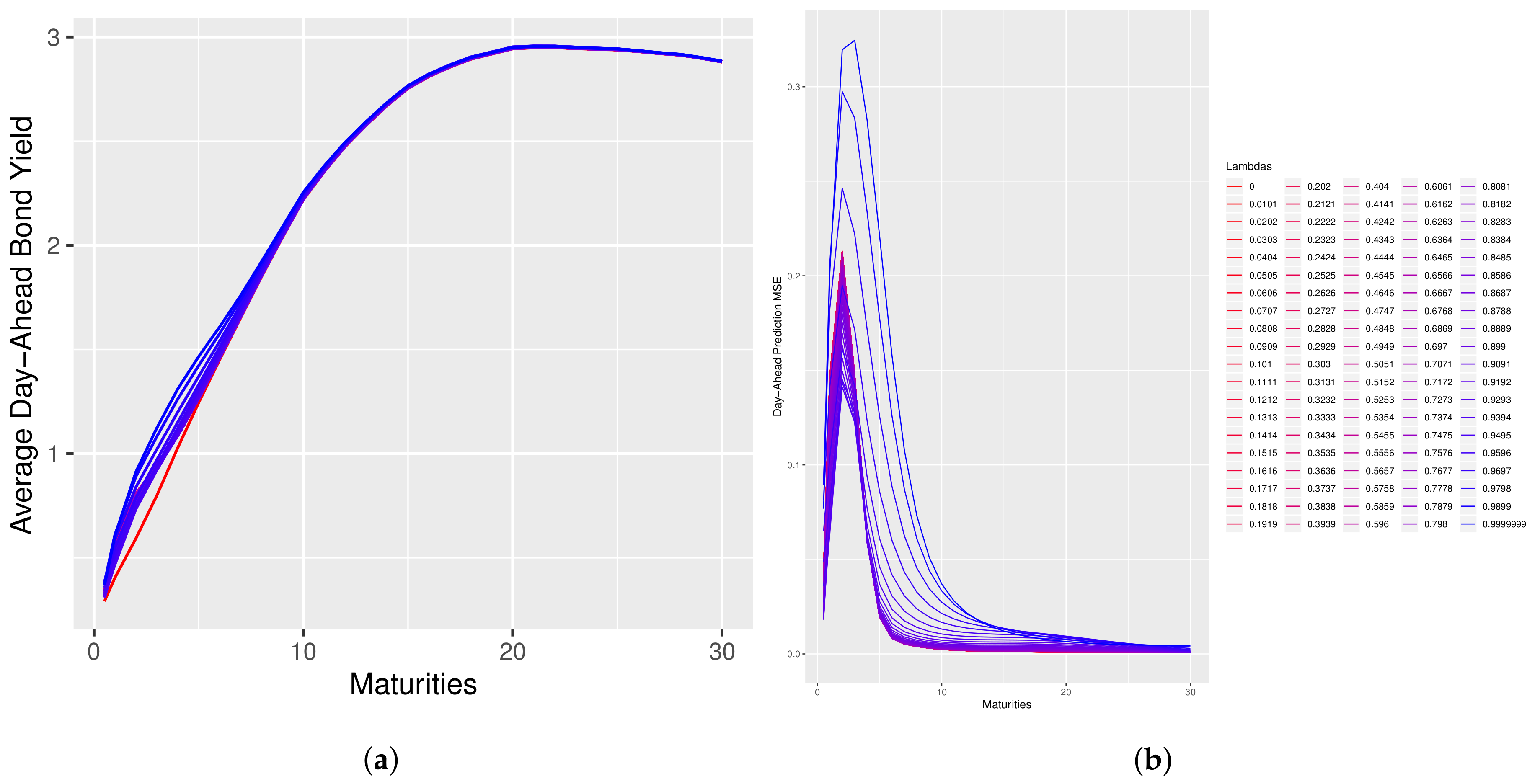
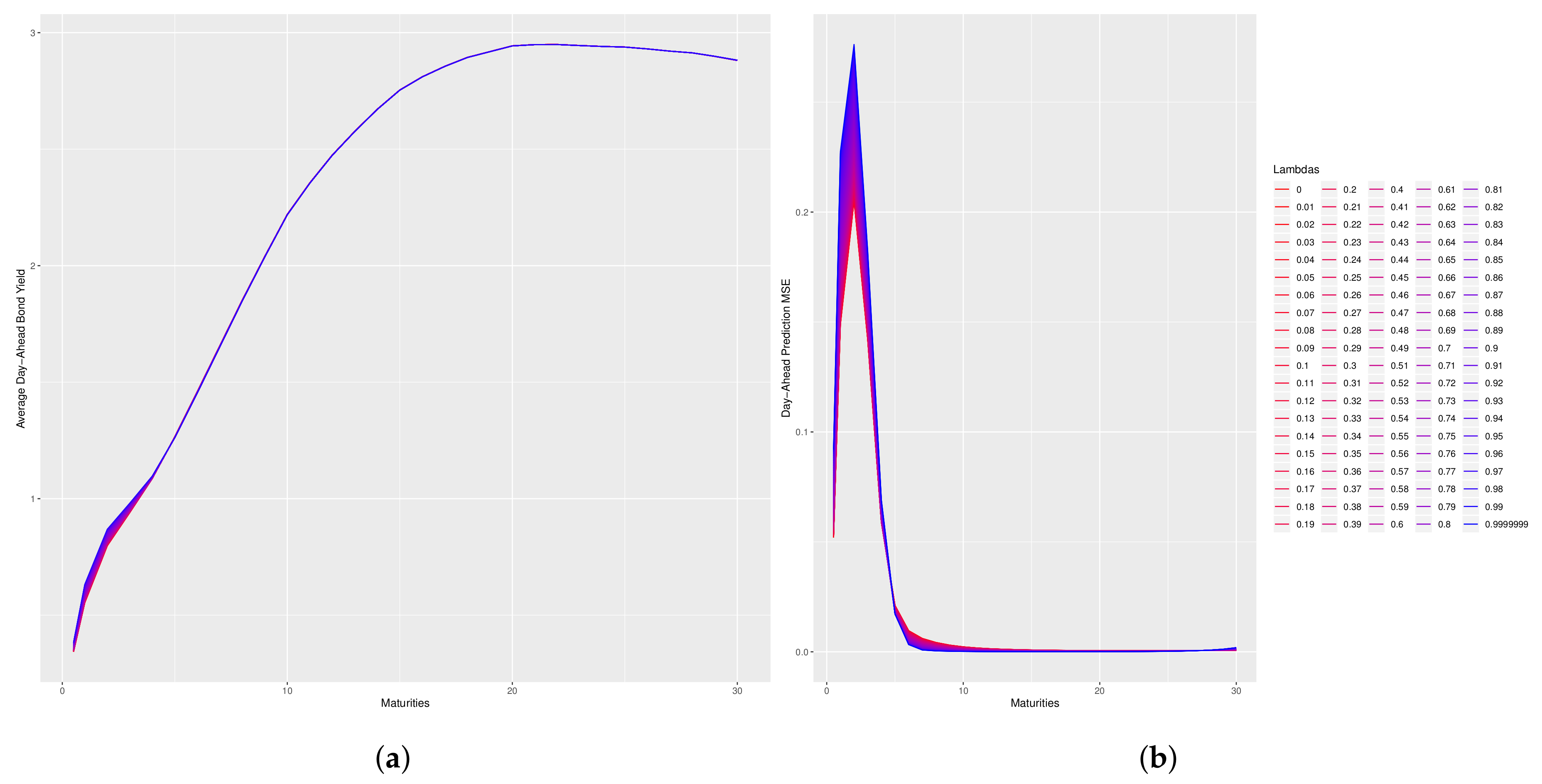
Unlike most regularization problems where there is a trade-off between the regularization term and the (un-regularized) objective function, the arbitrage-regularization requires $\lambda$ to be taken as close to 1 as possible. Since the limit (26) can only be approximated numerically $\lambda$ cannot be evaluated, however $\lambda$ can be taken to be arbitrarily close to, but less than, 1. This choice is justified by Figure 1 and Figure 2 which illustrates that for values of $\lambda$ near 1 there is little change in the model’s predictive performance.

Figure 1 and Figure 2 plot the change in the shape of the day-ahead predicted forward-rate curve and the change in the MSE of the day-ahead predicted bond prices as function of $\lambda$. In those figures, the curves with a pink color correspond to low values of $\lambda$ and the curves progressing towards a blue color correspond to high values of lambda. Please note that in these plots, the reparameterization of Corollary 1 is used and an abuse of notation is made by using $\lambda$ to denote $\tilde{\lambda }$.

In the case of the dNS model, an interesting property is that long-maturity bond prices do not change much, whereas short-maturity bond prices exhibit more dramatic changes. This property suggests that the dNS model is closer to being arbitrage-free on the long end of the curve than it is on the short end. This paper introduced a novel model-selection problem and provided an asymptotic solution in the form of the penalized optimization given by problem (9). The problem was posed and solved in a generalized HJM-type setting, within Theorem 1 and specialized to the term-structure of interest setting in Theorem 2 where simple expressions for the penalty term were derived.

The key innovation of the paper was the construction of the penalty term ${\mathrm{AF}}^{\lambda }$ defining the arbitrage-regularization problem (9). The construction of this term in Proposition 1 relied on the structure of the generalized HJM-type setting proposed in Heath et al. (1992) and generalized in (4) which allowed one to encode the dynamics of a large class of factor models with stochastic inputs into the specific structure of any asset class.

The numerical feasibility of the proposed method was made possible by the flexibility of feed-forward neural networks, as demonstrated in Hornik (1991); Kratsios (2019b), which allowed the optimizer of the arbitrage-regularization problem (9) to be approximated to arbitrary precision. In the numerics section of this paper, it was found that the arbitrage-regularization of a factor model does not heavily impact its predictive performance but does make it approximately consistent with no-arbitrage requirements.

In particular, the compatibility of the proposed approach with generic factor models with stochastic inputs allowed for the consistent use of factor models generated from machine learning methods. The A-Reg(dPCA) model is a novel example of such an approximately arbitrage-free model where the dynamics and factors were generated algorithmically instead of through practitioner experience.

The precise quantification of the approximate arbitrage-free property was made in Proposition 2. Thus, approximately arbitrage-free factor models under the stylized assumption of no transaction costs were indeed arbitrage-free when proportional transaction costs are in place, which is a more realistic assumption.

Finally, the arbitrage-regularization approach introduced in this paper opens the door to the compatible use of predictive machine-learning factor models with the no-free lunch with vanishing risk condition. The general treatment in Theorem 1 can be transferred to other asset classes and models generated from other learning algorithms. This approach can be an important new avenue of research lying at the junction of predictive machine learning and mathematical finance.

References

1. Bachelier, Louis. 1900. Théorie de la spéculation. Annales Scientifiques de l’É.N.S. 17: 21–86. [Google Scholar] [CrossRef]
2. Bain, Alan, and Dan Crisan. 2009. Fundamentals of stochastic filtering. In Stochastic Modelling and Applied Probability. New York: Springer, vol. 60. [Google Scholar]
3. Björk, Tomas. 2009. Arbitrage Theory in Continuous Time, 3rd ed. Oxford: Oxford University Press. [Google Scholar]
4. Björk, Tomas, and Bent Jesper Christensen. 1999. Interest rate dynamics and consistent forward rate curves. Mathematical Finance 9: 323–48. [Google Scholar] [CrossRef]
5. Braides, Andrea. 2002. Γ-convergence for beginners. In Oxford Lecture Series in Mathematics and Its Applications. Oxford: Oxford University Press, vol. 22. [Google Scholar]
6. Brown, R. C., and Bohumir Opic. 1992. Embeddings of weighted Sobolev spaces into spaces of continuous functions. Proceedings of the Royal Society of London. Series A 439: 279–96. [Google Scholar]
7. Carmona, René. 2014. Springer Texts in Statistics. In Statistical Analysis of Financial Data in R, 2nd ed. Springer Texts in Statistics. New York: Springer. [Google Scholar]
8. Chen, Hung-Ching Justin, and Magdon-Ismail Malik. NN-OPT: Neural Network for Option Pricing Using Multinomial Tree. In International Conference on Neural Information Processing. New York: Springer, pp. 360–369.
9. Chen, Luyang, Markus Pelger, and Jason Zhu. 2019. Deep learning in asset pricing. Available online: https://ssrn.com/abstract=3350138 (accessed on 15 April 2020).
10. Christensen, Jens H. E., Francis X. Diebold, and Glenn D. Rudebusch. 2011a. The affine arbitrage-free class of Nelson-Siegel term structure models. Journal of Econometrics 164: 4–20. [Google Scholar] [CrossRef] [Green Version]
11. Cont, Rama, and David-Antoine Fournié. 2013. Functional Itô calculus and stochastic integral representation of martingales. Annals of Probability 41: 109–33. [Google Scholar] [CrossRef]
12. Cuchiero, Christa. 2011. Affine and Polynomial Processes. Ph.D. thesis, ETH Zurich, Zürich, Switzerland. [Google Scholar]
13. Cuchiero, Christa, Irene Klein, and Josef Teichmann. 2016. A new perspective on the fundamental theorem of asset pricing for large financial markets. Theory of Probability and Its Applications 60: 561–79. [Google Scholar] [CrossRef] [Green Version]
14. Dal Maso, Gianni. 1993. An introduction to Γ-convergence. In Progress in Nonlinear Differential Equations and Their Applications. Boston: Birkhäuser Boston, Inc., vol. 8. [Google Scholar]
15. De Giorgi, Ennio. 1975. Sulla convergenza di alcune successioni d’integrali del tipo dell’area. Rend. Mat. 8: 277–94. [Google Scholar]
16. Delbaen, Freddy, and Walter Schachermayer. 1994. A general version of the fundamental theorem of asset pricing. Mathematische Annalen 300: 463–520. [Google Scholar] [CrossRef]
17. Delbaen, Freddy, and Walter Schachermayer. 1998. The fundamental theorem of asset pricing for unbounded stochastic processes. Mathematische Annalen 312: 215–50. [Google Scholar] [CrossRef] [Green Version]
18. Devin, Siobhán, Bernard Hanzon, and Thomas Ribarits. 2010. A Finite-Dimensional HJM Model: How Important is Arbitrage-Free Evolution? International Journal of Theoretical and Applied Finance 13: 1241–63. [Google Scholar] [CrossRef]
19. Diebold, Francis X., and Glenn D. Rudebusch. 2013. Yield Curve Modeling And Forecasting. Princeton: Princeton University Press. [Google Scholar]
20. Dupire, Bruno. 2009. Functional Itô Calculus. Bloomberg Portfolio Research Paper No. 2009-04-FRONTIERS. New York: Bloomberg L.P. [Google Scholar]
21. Elworthy, K. David. 1982. Stochastic Differential Equations on Manifolds. London Mathematical Society Lecture Note Series; Cambridge: Cambridge University Press, vol. 70. [Google Scholar]
22. Filipović, Damir. 2000. Exponential-polynomial families and the term structure of interest rates. Bernoulli 6: 1081–107. [Google Scholar] [CrossRef]
23. Filipović, Damir. 2001. Consistency Problems for Heath-Jarrow-Morton Interest Rate Models. Lecture Notes in Mathematics. Berlin: Springer, vol. 1760. [Google Scholar]
24. Filipović, Damir. 2009. Term-Structure Models. A Graduate Course. Springer Finance. Berlin: Springer. [Google Scholar]
25. Filipović, Damir, Stefan Tappe, and Josef Teichmann. 2010. Term structure models driven by Wiener processes and Poisson measures: Existence and positivity. SIAM Journal on Financial Mathematics 1: 523–54. [Google Scholar] [CrossRef] [Green Version]
26. Filipović, Damir, and Josef Teichmann. 2004. On the geometry of the term structure of interest rates. Proceedings of the Royal Society of London A: Mathematical, Physical and Engineering Sciences 460: 129–67. [Google Scholar] [CrossRef] [Green Version]
27. Focardi, Matteo. 2012. Γ-convergence: A tool to investigate physical phenomena across scales. Mathematical Methods in the Applied Sciences 35: 1613–58. [Google Scholar] [CrossRef]
28. Fontana, Claudio. 2014. A note on arbitrage, approximate arbitrage and the fundamental theorem of asset pricing. Stochastics An International Journal of Probability and Stochastic Processes 86: 922–31. [Google Scholar] [CrossRef] [Green Version]
29. Fournie, David-Antoine. 2010. Functional Ito Calculus and Applications. Ph.D. thesis, Columbia University, New York, NY, USA. [Google Scholar]
30. Gelenbe, Erol. 1989. Random neural networks with negative and positive signals and product form solution. Neural Computation 1: 502–10. [Google Scholar] [CrossRef]
31. Gonon, Lukas, Lyudmila Grigoryeva, and Juan-Pablo Ortega. 2020. Approximation bounds for random neural networks and reservoir systems. arXiv arXiv:2002.05933. [Google Scholar]
32. Guasoni, Paolo. 2006. No arbitrage under transaction costs, with fractional Brownian motion and beyond. Mathematical Finance 16: 569–82. [Google Scholar] [CrossRef]
33. Harrison, J. Michael, and David M. Kreps. 1979. Martingales and arbitrage in multiperiod securities markets. Journal of Economic Theory 20: 381–408. [Google Scholar] [CrossRef]
34. Hastie, Trevor, Robert Tibshirani, and Martin Wainwright. 2015. Statistical Learning with Sparsity: The LASSO and Generalizations. Boca Raton: CRC Press. [Google Scholar]
35. Heath, David, Robert Jarrow, and Andrew Morton. 1992. Bond Pricing and the Term Structure of Interest Rates: A New Methodology for Contingent Claims Valuation. Econometrica 60: 77–105. [Google Scholar] [CrossRef]
36. Hornik, Kurt. 1991. Approximation capabilities of multilayer feedforward networks. Neural Networks 4: 251–57. [Google Scholar] [CrossRef]
37. Jaeger, Herbert, and Harald Haas. 2004. Harnessing nonlinearity: Predicting chaotic systems and saving energy in wireless communication. Science 304: 78–80. [Google Scholar] [CrossRef] [PubMed] [Green Version]
38. Jazaerli, Samy, and Yuri F. Saporito. 2017. Functional Itô calculus, Path-Dependence and the Computation of Greeks. Stochastic Processes and their Applications 127: 3997–4028. [Google Scholar] [CrossRef] [Green Version]
39. Kratsios, Anastasis. 2019a. Deep Arbitrage-Free Regularization. Available online: https://github.com/AnastasisKratsios/Deep_Arbitrage_Free_Regularization/ (accessed on 8 April 2020).
40. Kratsios, Anastasis. 2020. The Universal Approximation Property: Characterizations, Existence, and a Canonical Topology for Deep-Learning. Machine Learning arXiv:1910.03344. [Google Scholar]
41. Meucci, Attilio. 2005. Risk and Asset Allocation. Springer Finance. Berlin: Springer. [Google Scholar]
42. Musiela, Marek, and Marek Rutkowski. 1997. Martingale Methods in Financial Modelling. In Applications of Mathematics. Berlin: Springer, vol. xii, p. 512. [Google Scholar]
43. Nelson, Charles R., and Andrew F. Siegel. 1987. Parsimonious modeling of yield curves. Journal of Business 60: 473–89. [Google Scholar] [CrossRef]
44. Pang, Tao, and Azmat Hussain. 2015. An application of functional Ito’s formula to stochastic portfolio optimization with bounded memory. In Paper presented at 2015 Proceedings of the Conference on Control and Its Applications, Paris, France, July 8–10; pp. 159–166. [Google Scholar]
45. Rahimi, Ali, and Benjamin Recht. 2008. Random features for large-scale kernel machines. In Advances in Neural Information Processing Systems. Vancouver: NIPS, pp. 1177–1184. [Google Scholar]
46. Schweizer, Martin. 1995. On the minimal martingale measure and the Föllmer-Schweizer decomposition. Stochastic Analysis and Applications 13: 573–99. [Google Scholar] [CrossRef]
47. Shreve, Steven E. 2004. Stochastic Calculus for finance II: Continuous-Time Models. Berlin: Springer Science & Business Media, vol. 11. [Google Scholar]
48. Tibshirani, Robert. 1996. Regression shrinkage and selection via the LASSO. Journal of the Royal Statistical Society. Series B (Methodological) 58: 267–88. [Google Scholar] [CrossRef]
49. Zou, Hui, Trevor Hastie, and Robert Tibshirani. 2006. Sparse principal component analysis. Journal of Computational and Graphical Statistics 15: 265–86. [Google Scholar] [CrossRef] [Green Version]
Sample Availability: Code is available at: https://github.com/AnastasisKratsios.
Figure 1. Day-ahead predictions as a function of λ ˜ across given maturities for the A−Reg(dNS) model. (a) Average day-ahead predicted yield curves. (b) Estimated MSE of day-ahead bond price predictions.
Risks 08 00040 g001
Figure 2. Day-ahead predictions as a function of λ ˜ across given maturities for the A−Reg(dPCA) model. (a) Average day-ahead predicted yield curves. (b) Estimated MSE of day-ahead bond price predictions.
Risks 08 00040 g002