Article

Machine Learning for Multiple Yield Curve Markets: Fast Calibration in the Gaussian Affine Framework

Department of Mathematical Stochastics, University of Freiburg, Ernst-Zermelo Str. 1, 79104 Freiburg im Breisgau, Germany
*
Author to whom correspondence should be addressed.
Risks 2020, 8(2), 50; https://doi.org/10.3390/risks8020050
Submission received: 16 April 2020 / Revised: 12 May 2020 / Accepted: 13 May 2020 / Published: 21 May 2020
(This article belongs to the Special Issue Machine Learning in Finance, Insurance and Risk Management)

Abstract

:
Calibration is a highly challenging task, in particular in multiple yield curve markets. This paper is a first attempt to study the chances and challenges of the application of machine learning techniques for this. We employ Gaussian process regression, a machine learning methodology having many similarities with extended Kálmán filtering, which has been applied many times to interest rate markets and term structure models. We find very good results for the single-curve markets and many challenges for the multi-curve markets in a Vasiček framework. The Gaussian process regression is implemented with the Adam optimizer and the non-linear conjugate gradient method, where the latter performs best. We also point towards future research.

1. Introduction

It is the aim of this paper to apply machine learning techniques to the calibration of bond prices in multi-curve markets in order to predict the term structure of basic instruments. The challenges are two-fold: On the one side, interest rate markets are characterized by having not only single instruments, such as stocks, but also full term structures, i.e., the curve of yields for different investment periods. On the other side, in multi-curve markets, not only one term structure is present but multiple yield curves for different lengths of the future investment period are given in the market and have to be calibrated. This is a very challenging task (see Eberlein et al. (2019) for an example using Lévy processes).
The co-existence of different yield curves associated to different tenors is a phenomenon in interest rate markets which originates with the 2007–2009 financial crisis. In this time, spreads between different yield curves reached their peak beyond 200 basis points. Since then, the spreads have remained on a non-negligible level. The most important curves to be considered in the current economic environment are the overnight indexed swap (OIS) rates and the interbank offered rates (abbreviated as Ibor, such as Libor rates from the London interbank market) of various tenors. In the European market, these are, respectively, the Eonia-based OIS rates and the Euribor rates. The literature on multiple yield curves is manifold and we refer to the works of Grbac and Runggaldier (2015) and Henrard (2014) for an overview. The general theory and affine models have been developed and applied, among others, in Grbac et al. (2016, 2019); Fontana et al. (2020); Grbac et al. (2015); Mercurio (2010).
The recent developments have seen many machine learning techniques, in particular deep learning became very popular. While deep learning typically needs big data, here we are more confronted with small data together with a high-dimensional prediction problem, since a full curve (the term structure), and in the multi-curve market, even multiple curves have to be calibrated and predicted. To be able to deal with this efficiently, one would like to incorporate information from the past, and a Bayesian approach seems best suited to this. We choose Gaussian process regression (GPR) as our machine learning approach which ensures fast calibration (see De Spiegeleer et al. (2018)). This is a non-parametric Bayesian approach to regression and is able to capture non-linear relationships between variables. The task of learning in Gaussian processes simplifies to determining suitable properties for the covariance and mean function, which determine the calibration of our model. We place ourselves in the context of the Vasiček model, which is a famous affine model (see the works of Filipović (2009) and Keller-Ressel et al. (2018) for a guide to the literature and details.)
It is generally accepted that machine learning performs better with higher-dimensional data. In a calibration framework such as the one we are studying here with GPR, it turns out that this seems not to be the case. While we find very good results for the single-curve markets, we find many challenges for the multi-curve markets in a Vasiček framework. A possible reason for this is that, in the small data setting considered here, the GPR is not able to exploit sparseness in the data.

Related Literature

Calibration of log-bond prices in the simple Vasiček model framework via Gaussian processes for machine learning has already been applied in Beleza Sousa et al. (2012) for a single maturity and in Beleza Sousa et al. (2014) for several maturities. They both rely on the theory of Gaussian processes presented in Rasmussen and Williams (2006). While in Section 3 we extend Beleza Sousa et al. (2012) by presenting an additional optimization method, Beleza Sousa et al. (2014) and Section 4 constitute a different access to the calibration of interest rate markets with several maturities. While Beleza Sousa et al. (2014) calibrated solely zero-coupon log-bond prices, from which one is not able to construct a post-crisis multi-curve interest rate market, we calibrate zero-coupon log-bond prices and log- δ -bond prices on top in order to encompass forward rate agreements and to be conform with the multi-curve framework (cf. Fontana et al. (2020) for the notion of δ -bonds). The modeling of log- δ -bond prices allows building forward-rate-agreements (FRAs) so that we have the basic building blocks for multi-curve interest rate markets.

2. Gaussian Process Regression

Following Rasmussen and Williams (2006, chps. 2 and 5), we provide a brief introduction to Gaussian process regression (GPR). For a moment, consider a regression problem with additive Gaussian noise: we observe y 1 , , y n together with covariates x 1 , , x n and assume that
y i = f ( x i , θ ) + ϵ i , i = 1 , , n ,
where f ( · , θ ) is a regression function depending on the unknown parameter θ and ϵ is a d-dimensional noise vector which we assume to consist of i.i.d. mean-zero Gaussian errors and standard deviation σ ^ .
In the Bayesian approach, we are not left without any knowledge on θ but may start from a prior distribution; sometimes this distribution can be deducted from previous experience in similar experiments, while otherwise one chooses an uninformative prior. Assuming continuity of the prior, we denote the prior density of θ by p ( θ ) . Inference is now performed by computing the a posteriori distribution of θ conditional on the observation ( x , y ) . This can be achieved by Bayes’ rule, i.e.,
p ( θ | x , y ) = p ( θ , y | x ) p ( y | x ) = p ( y | x , θ ) p ( θ ) p ( y | x ) ,
where we assume only that the distribution of θ does not depend on x. Similarly, we can compute p ( y | x ) from p ( y | x , θ ) by integrating with respect to p ( θ ) .
For a moment, we drop the dependence on x in the notation. Assuming only that the observation y N ( μ y , Σ y y ) is normally distributed, we are already able to state the marginal likelihood p ( y ) : it is given up to a normalizing constant c by
log p ( y ) = c 1 2 ( y μ y ) Σ y y 1 ( y μ y ) .
If we assume moreover that ξ = f ( θ ) is jointly normally distributed with y, we arrive at the multivariate Gaussian case. Hence, the conditional distribution p ( ξ | x , y ) is again Gaussian and can be computed explicitly. Starting from ( ξ , y ) N ( μ , Σ ) , where we split μ = ( μ ξ , μ y ) and
Σ = Σ ξ ξ Σ ξ y Σ y ξ Σ y y ,
we can compute p ( ξ | y ) through some straightforward calculations. First, observe that y N ( μ y , Σ ξ ξ + σ ^ 2 I n ) . We obtain Σ y y = Σ ξ ξ + σ ^ 2 I n . Hence, the marginal likelihood is given by
log p ( y ) = c ˜ 1 2 ( y μ y ) Σ ξ ξ + σ ^ 2 I n 1 ( y μ y ) .
Second, we compute
ξ | y N μ ξ + Σ ξ y Σ y y 1 ( y μ y ) , Σ ξ ξ Σ ξ y Σ y y 1 Σ y ξ .
This formula is the basis for the calibration in the Vasiček model, as we show now.

3. The Single-Curve Vasiček Interest Rate Model

As a first step, we calibrate the single-curve Vasiček interest rate model following Beleza Sousa et al. (2012). To begin with, we want to mention the important difference in mathematical finance between the objective measure P and the risk-neutral measure Q . The statistical propagation of all stochastic processes takes place under P . Arbitrage-free pricing means computing prices for options; of course, the prices depend on the driving stochastic factors. The fundamental theorem of asset pricing now yields that arbitrage-free prices of traded assets can be computed by taking expectations under a risk-neutral measure Q of the discounted pay-offs. For a calibration, the risk-neutral measure has to be fitted to observed option prices, which is our main target.
In this sense, we consider zero-coupon bond prices under the risk-neutral measure Q . The Vasiček model is a single-factor model driven by the short rate r = ( r t ) t 0 which is given by the solution of the stochastic differential equation
d r t = κ ( θ r t ) d t + σ d W t , t 0 ,
with initial value r 0 . Here, W is a Q -Brownian motion and κ , θ , σ are positive constants. For a positive κ , the process r converges to the long-term mean θ .
The price process of the zero-coupon bond price with maturity T is denoted by ( P ( t , T ) ) 0 t T with P ( T , T ) = 1 . The Vasiček model is an affine bond price model, which implies that bond prices take an exponential affine form, i.e.,
P ( t , T ) = e A ( T t ) B ( T t ) r t for t T .
Here, the functions ( A ( · ) , B ( · ) ) : [ 0 , T ] R × R are given by
A ( T t ) = θ κ e κ ( T t ) + κ ( T t ) 1 + σ 2 4 κ 3 e 2 κ ( T t ) 4 e κ ( T t ) 2 κ ( T t ) + 3 , B ( T t ) = 1 κ ( 1 e κ ( T t ) ) .
We recall that the solution of the stochastic differential Equation (4) is given by (cf. Brigo and Mercurio (2001, chp. 4.2)),
r t = r 0 e κ t + θ ( 1 e κ t ) + σ e κ t 0 t e κ u d W u .
Together with Equation (5), this implies that the zero coupon bond prices are log-normally distributed. To apply the Gaussian process regression, we consider in the sequel log-bond prices for t T ,
y ( t , T ) = log P ( t , T ) = A ( T t ) B ( T t ) r t .
The corresponding mean function is given by
μ ( t , T ) : = E Q log P ( t , T ) = A ( T t ) B ( T t ) r 0 e κ t + θ ( 1 e κ t ) ,
and the covariance function is given by
c ( s , t , T ) : = E Q log P ( s , T ) E Q [ log P ( s , T ) ] · log P ( t , T ) E Q [ log P ( t , T ) ] = B ( T s ) B ( T t ) E Q [ r s r t ] E Q [ r s ] E Q [ r t ] = B ( T s ) B ( T t ) σ 2 2 κ e κ ( s + t ) ( e 2 κ ( s t ) 1 ) .
An observation now consists of a vector y = ( y ( t 1 , T ) , , y ( t n , T ) ) + ϵ of log-bond prices with additional Gaussian i.i.d. noise with variance σ ^ 2 . Consequently, y N ( μ y , Σ y y ) with
μ y = ( μ ( t 1 , T ) , , μ ( t n , T ) ) ( Σ y y ) i , j = c ( t i , t j , T ) + σ ^ 2 1 { i = j } .
We define the vector of hyper-parameters as Θ = ( r 0 , κ , θ , σ ) and aim at finding the most reasonable values of hyper-parameters, minimizing the negative log marginal likelihood defined in Equation (1) with the underlying mean covariance function from Equation (9).
Remark 1.
[Extending the observation] Note that, in the set-up considered here, the driving single factor process r is considered not observable at t 0 , t 1 , , t n ; compare Equation (9) which depends on r 0 only (and on Θ of course). Such an approach may be appropriate for short time intervals. The propagation of r 0 to the future times t 1 , , t n is solely based on the risk-neutral evolution under the risk-neutral measure Q via μ and c.
If, on the contrary, updating of r should be incorporated, the situation gets more complicated since the evolution of r (taking place under the statistical measure P ) needs to be taken into account. One can pragmatically proceed as follows: assume that at each time point r is observable. We neglect the information contained in this observation about the hyper-parameters Θ. Then, the formulas need to be modified only slightly by using conditional expressions. For example, μ ( t , T ) conditional on r s for s t equals
E Q [ log P ( t , T ) | r s ] = A ( T t ) B ( T t ) ( r s e κ ( t s ) + θ ( 1 e κ ( t s ) ) ) ,
and, if t = s , this simplifies even further.
In a similar spirit, one may extend the observation by adding bond prices with different maturities or, additionally, derivatives. A classical calibration example would be the fitting of the hyper-parameters to the observation of bond prices and derivatives, both with different maturities, at a fixed time t 0 . The Gaussian process regression hence also provides a suitable approach for this task. We refer to De Spiegeleer et al. (2018) for an extensive calibration example in this regard.
We refer to Rasmussen and Williams (2006) for other approaches to model selection such as cross validation or alignment. For our application purposes, maximizing the log-marginal likelihood is a good choice since we already have information about the choice of covariance structure, and it only remains to optimize the hyper-parameters (cf. Fischer et al. (2016)).

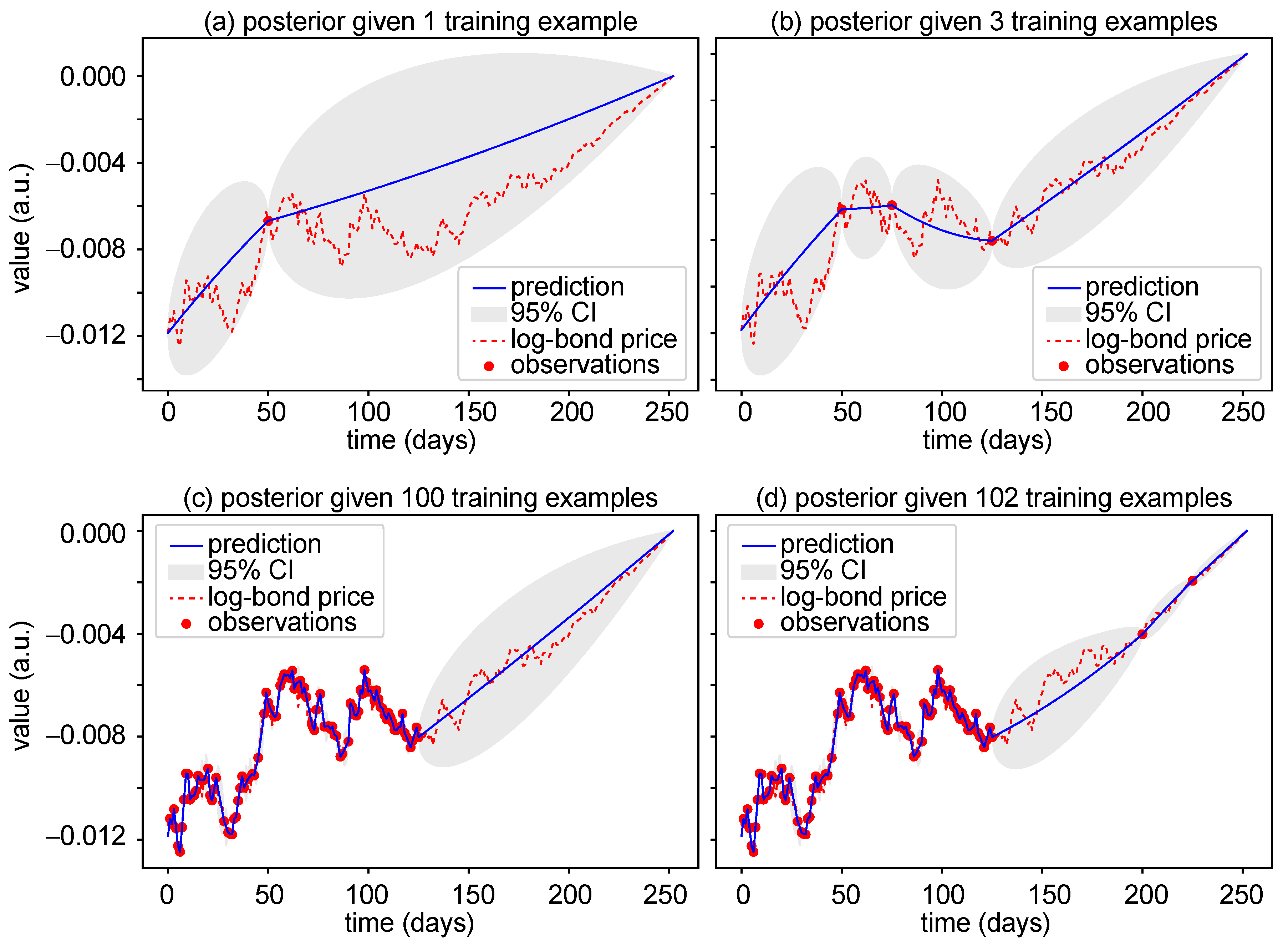
3.1. Prediction with Gaussian Processes Regression

The prediction of new log-bond prices given some training data is of interest in the context of the risk management of portfolios and options on zero-coupon bonds and other interest derivatives. The application to pricing can be done along the lines of Dümbgen and Rogers (2014), which we do not deepen here. Once having found the calibrated parameters Θ , we can apply those calibrated parameters to make predictions for new input data.
For the dynamic prediction of log-bond prices, we seek a function that is able to predict new output values given some new input values, initially based on a set of training data. For this purpose, we specify in a first step the prior distribution, expressing our prior beliefs over the function. In Figure 1, we plot for the sake of illustration one simulated log-bond price and an arbitrary chosen prior, expressing our beliefs. This could correspond to the log-prices of a one-year maturity bond, plotted over 252 days. The blue line constitutes the prior mean and the shaded area nearly twice the prior standard deviation corresponding to the 95% confidence interval (CI). Without observing any training data, we are able to neither narrow the CI of our prior nor enhance our prediction.
The next step is to incorporate a set of training data, to enhance our prediction. The Gaussian process regression has a quite fascinating property in this regard: consider an observation at the time point t, t { 1 , , 251 } . The prediction for y ( t ) is of course y ( t ) itself—and hence perfect. The prediction of y ( s ) , be it for s < t (which is often called smoothing) or the prediction for s > t (called filtering) is normally distributed, but, according to Equation (3), has a smaller variance compared to our initial prediction without the observation of y ( t ) . Increasing the number of observations to, e.g., y ( t 1 ) , , y ( t n ) improves the prediction dramatically. We illustrate this property in Figure 2. Depending on the location of s relative to t 1 , , t n , the prediction can become very exact (bottom right-for s [ 0 , 130 ] ) and may still have a significant error (e.g., for s around 180).
We now formalize the question precisely: given some training data y = ( y ( t 1 , T ) , , y ( t n , T ) ) we aim at predicting the vector y ˜ = ( y ( s 1 , T ) , , y ( s m , T ) ) .
The joint distribution of y and y ˜ can directly be obtained from the mean and covariance functions in Equations (7) and (8): since they are jointly normally distributed, we obtain that
y y ˜ N μ y μ y ˜ , Σ y y Σ y y ˜ Σ y ˜ y Σ y ˜ y ˜ .
Recall that μ y and Σ y y are already specified in Equation (9). Analogously, we obtain that
( μ y ˜ ) i = μ ( s i , T ) ( Σ y y ˜ ) i , j = c ( t i , s j , T ) ( Σ y ˜ y ) i , j = c ( s i , t j , T ) ( Σ y ˜ y ˜ ) i , j = c ( s i , s j , T ) .
The posterior distribution is obtained by using Equation (3): conditional on the training data y, we obtain that
y ˜ | y N μ ˜ , Σ ˜ ,
where
μ ˜ = μ y ˜ + Σ y ˜ y Σ y y 1 ( y μ y )
and
Σ ˜ = Σ y ˜ y ˜ Σ y ˜ y Σ y y 1 Σ y y ˜ .
Given some training data, Equation (10) now allows calculating the posterior distribution, i.e., the conditional distribution of the predictions y ˜ given the observation y, and to make predictions, derive confidence intervals, etc.
The posterior distributions, i.e., the prior conditioned on some training data of 1, 3, 100, and 102 observations, respectively, is shown in Figure 2. The red dotted line represents a simulated trajectory of the log-bond price, while the red dots constitute the observed training data. The blue line is the posterior mean, which we take as our prediction, and the shaded areas denote the 95% confidence interval (CI). We observe that the more training data we have, the more accurate our prediction gets. While in Figure 2a the CI is quite large, two additional training data narrow the CI significantly down (see Figure 2b). Of course, the observation times t i play an important role in this: if we had observations t i close to t i 1 , the additional gain in knowledge would most likely be small, while, in Figure 2b, the ( t i ) are nicely spread. Consequently, if one is able to choose the ( t i ) , one can apply results from optimal experimental design to achieve a highly efficient reduction in the prediction variance.
In most practical cases, the ( t i ) cannot be chosen freely, and just arrive sequentially, as we illustrate in Figure 2c,d: here, we aim at predicting log-bond prices of a one-year maturity bond which we have observed daily until day t n = 125 . Figure 2c describes the situation in which we do not have any information about future prices of the one-year maturity bond, i.e., the second half of the one year. Figure 2d depicts the situation in which we assume to know two log-bond prices or option strikes on zero-coupon bonds in the future, which enhances the prediction and narrows the CI down.

3.2. Performance Measures

To monitor the performance of the calibration or the prediction, one typically splits the observed dataset into two disjoint sets. The first set is called training set and is used to fit the model. The second is the validation set and used as a proxy for the generalization error. Given the number of observed data points and number of parameters to optimize for our simulation task, we recommend splitting the training and validation test set in a 70 % / 30 % ratio. The quality of the predictions can be assessed with the standardized mean squared error (SMSE) loss and the mean standardized log loss (MSLL).
The SMSE considers the average of the squared residual between the mean prediction and the target of the test set and then standardizes it by the variance of the targets of the test cases.
SMSE = 1 σ ˜ 2 1 m i = 1 m ( y ˜ i μ ˜ i ) 2 ,
where σ ˜ 2 denotes the variance of the targets of the test cases. The SMSE is a simple approach and the reader should bear in mind that this assessment of the quality does not incorporate information about the predictive variance. However, as it represents a standard measure of the quality of an estimator, it is useful to consider it for the sake of comparability with other literature.
The MSLL as defined in Rasmussen and Williams (2006) is obtained by averaging the negative log probability of the target under the model over the test set and then standardizing it by subtracting the loss that would be obtained under the trivial model with mean and variance of the training data as in Equation (1),
MSLL = 1 m i = 1 m log p ( y ˜ i | y ) + log p ( y ) .
The MSLL will be around zero for simple methods and negative for better methods. Note that in Equation (11) we omit in the notation the dependence on the parameter set Θ , since now the parameter set is fixed. Moreover, we notice that the MSLL incorporates the predictive mean and the predictive variances unlike the SMSE.
In the following section, we simulate log-bond prices in a Vasiček single-curve model and calibrate the underlying parameters of the model. This is performed for one maturity. Since we deal with simulated prices, we consider the noise-free setting and set σ ^ 2 = 0 in Equation (2).

3.3. Calibration Results for the Vasiček Single-Curve Model

We generate 1000 samples of log-bond price time series, each sample consisting of 250 consecutive prices (approximately one year of trading time) via Equations (4) and (5). As parameter set, we fix
r 0 = 0.5 , κ = 2 , θ = 0.1 , σ = 0.2 .
For each of the 1000 samples, we seek the optimal choice of hyper-parameters Θ = { r 0 , κ , θ , σ } based on the simulated trajectory of 250 log-bond prices. For this purpose, we minimize the negative log marginal likelihood in Equation (1) with the underlying mean and covariance functions in Equations (7) and (8), respectively, by means of two optimization methods: the non-linear conjugate gradient (CG) algorithm and the adaptive moment estimation (Adam) optimization algorithm. The CG algorithm uses a non-linear conjugate gradient by Polak and Ribiere (1969). For details on the CG algorithm, we refer to Nocedal and Wright (2006). The Adam optimization algorithm is based on adaptive estimates of lower-order moments and is an extension of the stochastic gradient descent. For details of the Adam optimization algorithm, we refer to Kingma and Ba (2014).
After a random initialization of the parameters to optimize, the CG optimization and the Adam optimization were performed using the Python library SciPy and TensorFlow, respectively. Parallelization of the 1000 independent runs was achieved with the Python library multiprocessing. The outcomes can be summarized as follows.
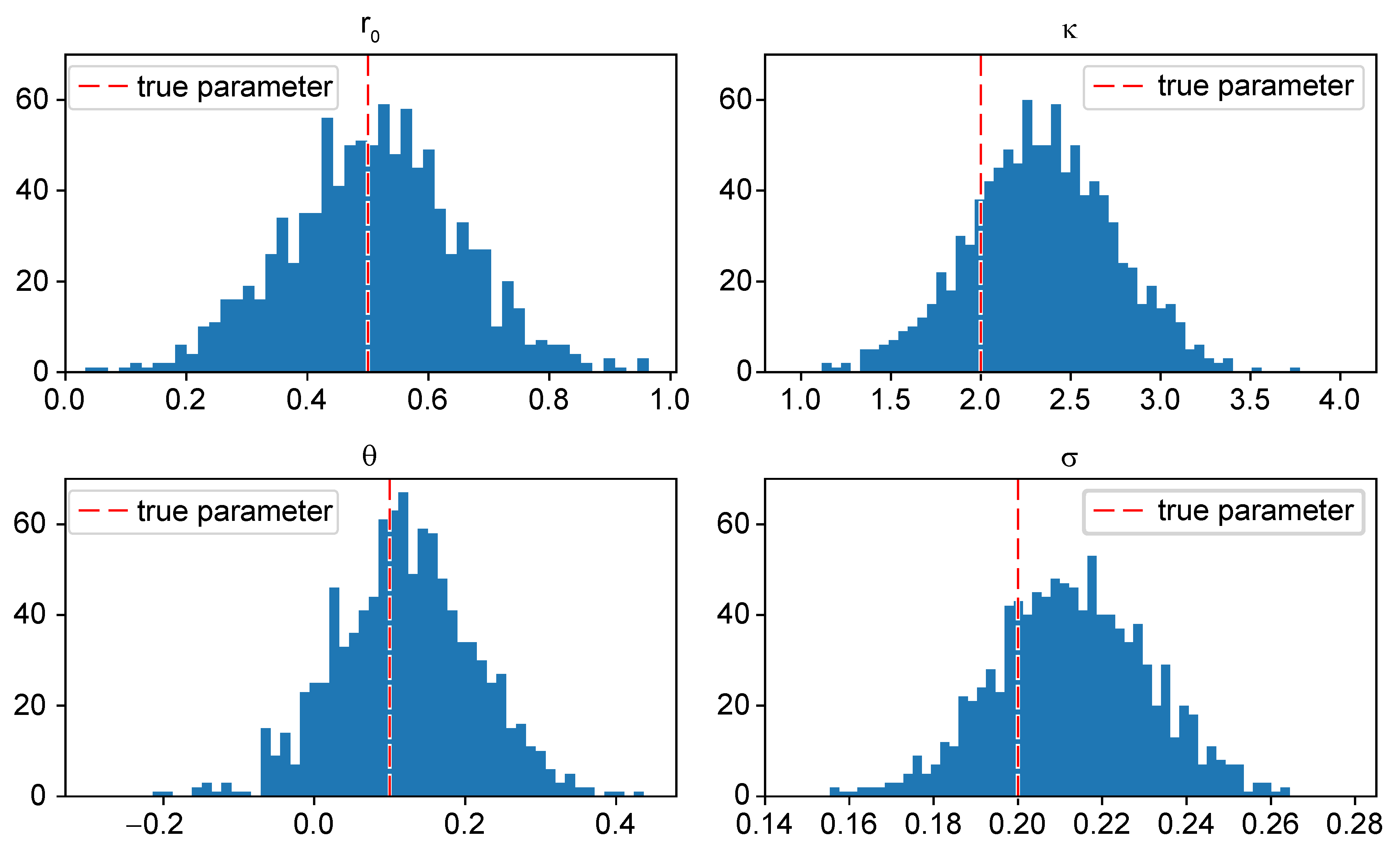
  • The results of the calibration via the conjugate gradient optimization algorithm are very satisfying. In Figure 3, the learned parameters r 0 , κ , θ , and σ of 1000 simulated log-bond prices are plotted in 50-bin histograms. The red dashed lines in each sub-plot indicate the true model parameters.
    The mean and standard deviation of the learned parameters are summarized in Table 1. We observe that the mean of the learned parameters reaches the true parameters very closely while the standard deviation is reasonable.
  • The results of the calibration via the Adam algorithm are satisfying, even though we note a shift of the mean reversion parameter κ and the volatility parameter σ . The learned parameters r 0 , κ , θ , and σ of 1000 simulated log-bond prices are plotted in 50-bin histograms in Figure 4 and summarized with their mean and standard deviation in Table 1. The Adam algorithm slowly reduces the learning rate over time to speed up the learning algorithm. Nonetheless, one needs to specify a suitable learning rate. If the learning rate is small, training is more reliable, but the optimization time to find a minimum can increase rapidly. If the learning rate is too big, the optimizer can overshoot a minimum. We tried different learning rates of 0.0001, 0.001, 0.01, 0.05, and 0.1. Finally, we decided in favor of a learning rate of 0.05 and performed the training over 700 epochs to achieve a suitable trade-off between accuracy and computation time. We expect the results to improve slightly with more epochs, at the expense of a longer training time.
We conclude that, in the single-curve Vasiček specification, both optimization algorithms provide reliable results. The optimization by means of the CG algorithm outperforms the Adam algorithm (see Table 1). However, there is hope that the results obtained by the Adam algorithm can be improved by increasing the number of training epochs or by choosing a smaller learning rate in addition to more training epochs.

4. Multi-Curve Vasiček Interest Rate Model

The financial crisis of 2007–2009 has triggered many changes in financial markets. In the post-crisis interest rate markets, multiple yield curves are standard: due to credit and liquidity issues, we obtain for each tenure a different curve (see, for example, Grbac and Runggaldier (2015) and the rich literature referenced therein).
The detailed mechanism in the multi-curve markets is quite involved, and we refer Fontana et al. (2020) for a precise description. Intuitively, traded instruments are forward-rate agreements which exchange a fixed premium against a floating rate over a future time interval [ T , T + δ ] . Most notably, in addition to the parameter maturity, a second parameter appears: the tenor δ . While before the crisis, the curves were independent of δ , after the crisis the tenure can no longer be neglected. The authors of Fontana et al. (2020) showed that forward-rate agreements can be decomposed into δ -bonds, which we denote by P ( t , T , δ ) . If δ = 0 we write P ( t , T ) = P ( t , T , 0 ) , which is the single-curve case considered previously.
In the multi-curve Vasiček interest rate model, we consider two maturity time points T T , hence δ = T T . We calibrate zero-coupon bond prices P ( t , T , 0 ) and tenor- δ -bond prices P ( t , T , δ ) under the risk-neutral measure Q at time t for the maturity T.
The calibration in the multi-curve framework corresponds to the situation in which we are given several datasets of different bond prices, where all of them are sharing the same hyper-parameters. We call this situation multi-task learning and reveal the different meaning in contrast to (Rasmussen and Williams 2006, sct. 5.4.3) where the corresponding log-marginal likelihoods of the individual problems are summed up and the result is then optimized with respect to the hyper-parameters. As our multi-curve example exhibits correlation, the latter approach cannot be applied.
We utilize a two-dimensional driving factor process r = ( r 1 , r 2 ) , generalizing Equation (4). Modeling r as a two-dimensional Ornstein–Uhlenbeck process can be done as follows: let r be the unique solution of the SDE
d r t i = κ i ( θ i r t i ) d t + σ i d W t i , t 0 , i = 1 , 2 ,
where W 1 , W 2 are two standard Q -Brownian motions with correlation ρ . The zero-coupon bond prices only depend on r 1 and we utilize the single-curve affine framework:
P ( t , T ) = e A ( T t ) B ( T t ) r t 1 for t T .
The functions ( A ( · ) , B ( · ) ) : [ 0 , T ] R × R satisfy again the Riccati equations. They are obtained from Equation (5) by replacing κ by κ 1 , etc. As in Equations (7) and (8), we obtain that zero-coupon log-bond prices y ( t , T , 0 ) = log P ( t , T , 0 ) are normal with mean function
μ ( t , T , 0 ) : = E Q log P ( t , T , 0 ) = A ( T t ) B ( T t ) r 0 1 e κ 1 t + θ 1 ( 1 e κ 1 t ) , t T
For two given time points t i , t j T , the covariance function is
c ( t i , t j , T , 0 ) : = B ( T t i ) B ( T t j ) σ 1 2 2 κ 1 e κ 1 ( t i + t j ) e 2 κ 1 ( t i t j ) 1 .
The next step is to develop the prices for the tenor- δ bonds. We assume that, while for the tenor 0 the interest rate is r 1 , the interest rate for tenor δ is r 1 + r 2 . This implies that P ( t , T , δ ) = E Q e t T ( r s 1 r s 2 ) d s | F t . Since r is an affine process, this expectation can be computed explicitly. Using the affine machinery, we obtain that
P ( t , T , δ ) = exp Φ ( T t ) + Ψ ( T t ) r t , for t T
where the function ( Φ ( · ) , Ψ ( · ) ) : [ 0 , T ] R × R 2 satisfies the Riccati equations. This implies that
Ψ 1 ( T t ) = B ( T t ) = 1 κ 1 1 e κ 1 ( T t ) , Ψ 2 ( T t ) = 1 κ 2 1 e κ 2 ( T t ) and Φ ( T t ) = ( θ 1 θ 2 ) ( T t ) θ 1 κ 1 e κ 1 ( T t ) 1 + θ 2 κ 2 e κ 2 ( T t ) 1 + σ 1 2 2 κ 1 2 T t + 2 κ 1 e κ 1 ( T t ) 1 2 κ 1 e 2 κ 1 ( T t ) 3 2 κ 1 + σ 2 2 2 κ 2 2 T t + 2 κ 2 e κ 2 ( T t ) 1 2 κ 2 e 2 κ 2 ( T t ) 3 2 κ 2 ρ σ 1 σ 2 κ 1 κ 2 ( T t + 1 κ 1 ( e κ 1 ( T t ) 1 ) + 1 κ 2 ( e κ 2 ( T t ) 1 ) 1 κ 1 + κ 2 e ( κ 1 + κ 2 ) ( T t ) 1 ) .
Proposition 2.
Under the above assumptions, log P ( · , T , δ ) , 0 t T is a Gaussian process with mean function
μ ( t , T , δ ) = Φ ( T t ) + Ψ 1 ( T t ) ( r 0 1 e κ 1 t + θ 1 ( 1 e κ 1 t ) ) + Ψ 2 ( T t ) ( r 0 2 e κ 2 t + θ 2 ( 1 e κ 2 t ) ) , t T ,
and with covariance function
c ( s , t , T , δ ) = Ψ 1 ( T s ) Ψ 1 ( T t ) σ 1 2 2 κ 1 e κ 1 ( s + t ) ( e 2 κ 1 ( s t ) 1 ) + Ψ 1 ( T s ) Ψ 2 ( T t ) ρ σ 1 σ 2 κ 1 + κ 2 e ( κ 1 s + κ 2 t ) ( e ( κ 1 + κ 2 ) ( s t ) 1 ) + Ψ 1 ( T t ) Ψ 2 ( T s ) ρ σ 1 σ 2 κ 1 + κ 2 e ( κ 1 t + κ 2 s ) ( e ( κ 1 + κ 2 ) ( t s ) 1 ) + Ψ 2 ( T s ) Ψ 2 ( T t ) σ 2 2 2 κ 2 e κ 2 ( s + t ) ( e 2 κ 2 ( s t ) 1 ) , 0 s , t T .
Note that μ and c in the above proposition do not depend on δ . We rather use δ as index to distinguish mean and covariance functions for the zero-coupon bonds and the δ -tenor bonds.
The proof is relegated to Appendix A. The next step is to phrase observation and prediction in the Gaussian setting explicitly. We denote y = ( y 0 , y δ ) where y 0 = ( y ( t 1 , T , 0 ) , , y ( t n , T , 0 ) ) and y δ = ( y ( t 1 , T , δ ) , , y ( t n , T , δ ) ) —of course, at each time point t i we observe two bond prices now: P ( t i , T , 0 ) and P ( t i , T , δ ) . The vector y is normally distributed, y N ( μ y , Σ y ) with
μ y : = μ ( · , T , 0 ) μ ( · , T , δ ) , Σ y : = Σ y 00 Σ y 0 δ Σ y δ 0 Σ y δ δ .
We calculate these parameters explicitly and, analogously to the single-curve set-up, the calibration methodology with Gaussian process regression follows.
To begin with, note that Σ y 00 coincides with Σ y y from Equation (9), when we replace the parameters r 0 , κ , θ , σ by r 0 1 , κ 1 , θ 1 , σ 1 , respectively. The next step for computing the covariance matrix is to compute
( Σ y 0 δ ) i , j : = E Q log P ( t i , T , 0 ) E Q log P ( t i , T , 0 ) · log P ( t j , T , δ ) E Q log P ( t j , T , δ ) = Ψ 1 ( T t i ) Ψ 1 ( T t j ) σ 1 2 2 κ 1 e κ 1 ( t i + t j ) ( e 2 κ 1 ( t i t j ) 1 ) + Ψ 1 ( T t i ) Ψ 2 ( T t j ) ρ σ 1 σ 2 κ 1 + κ 2 e ( κ 1 t i + κ 2 t j ) ( e ( κ 1 + κ 2 ) ( t i t j ) 1 ) ,
and, analogously,
( Σ y δ 0 ) i , j : = E Q log P ( t i , T , δ ) E Q log P ( t i , T , δ ) · log P ( t j , T , 0 ) E Q log P ( t j , T , 0 ) = Ψ 1 ( T t i ) Ψ 1 ( T t j ) σ 1 2 2 κ 1 e κ 1 ( t i + t j ) ( e 2 κ 1 ( t i t j ) 1 ) + Ψ 1 ( T t j ) Ψ 2 ( T t i ) ρ σ 1 σ 2 κ 1 + κ 2 e ( κ 1 t j + κ 2 t i ) ( e ( κ 1 + κ 2 ) ( t i t j ) 1 ) ;
in a similar way to Σ y 00 , we obtain Σ y δ δ .
In the multi-curve calibration, we aim at minimizing the log marginal likelihood in Equation (1) with the corresponding mean function and covariance matrix in Equation (18).

Calibration Results

For the calibration in the multi-curve setting, we have to consider log-bond prices and the logarithm of tenor- δ bond prices. To be specific, we generate 1000 sequences of log-bond prices and 1000 sequences of log tenor- δ bond prices with maturity 1 by means of Equations (13), (16), and (17). We choose as parameters
r 0 1 = 0.5 , κ 1 = 2 , θ 1 = 0.1 , σ 1 = 0.2 r 0 2 = 0.7 , κ 2 = 0.5 , θ 2 = 0.03 , σ 2 = 0.8 .
For each sequence, we generate 125 training data points of log-bond prices and 125 training data points of log tenor- δ bond prices. This corresponds to a computational effort similar to the single-curve specifications, since the underlying covariance matrix will be ( 250 × 250 ) -dimensional. Based on the simulated prices. we aim at finding the optimal choice of hyper-parameters
Θ = { r 0 1 , κ 1 , θ 1 , σ 1 , r 0 2 , κ 2 , θ 2 , σ 2 } .
For this purpose, we apply the CG optimization algorithm and the Adam optimization algorithm. After a random initialization of the parameters to optimize, we perform the calibration procedure using SciPy and TensorFlow for the CG and Adam optimizer, respectively. Parallelization of the 1000 independent runs is achieved with the library multiprocessing. The outcomes are as follows.
  • Considering the results of the calibration by means of the CG algorithm, we note several facts. In this regard, the mean and the standard deviation of the calibrated parameters can be found in Table 2. Figure 5 shows the learned parameters of the processes r 1 and r 2 in 50-bin histograms for 1000 simulations. The red dashed line in each of the sub-plots indicates the true model parameter value. First, except for the long term mean, the volatility for r 2 is higher than the one for r 1 . This implies more difficulties in the estimation of the parameters for r 2 , which is clearly visible in the results. For r 1 , we are able to estimate the parameters well (in the mean), with the most difficulty in the estimation of κ 1 which shows a high standard deviation. For estimating the parameters of r 2 , we face more difficulties, as expected. The standard deviation of θ 2 is very high—it is known from filtering theory and statistics that the mean is difficult to estimate, which is reflected here. Similarly, it seems difficult to estimate the speed of reversion parameter κ 2 and we observe a peak around 0.02 in κ 2 . This might be due to a local minimum, where the optimizer gets stuck.
  • For the calibration results by means of the Adam algorithm, we note the following. The learned parameters are illustrated in a 50-bin histogram (see Figure 6), and mean and standard deviation of each parameter are stated in Table 2. After trying several learning rates of 0.0001, 0.001, 0.01, 0.05, and 0.1, we decided in favor of the learning rate 0.05 and chose 750 training epochs. While most mean values of the learned parameters are not as close to the true values as the learned parameters from the CG algorithm, we notice that the standard deviation of the learned parameters is smaller compared to the standard deviation of the learned parameters from the CG. Especially, comparing the values of θ 2 in Figure 5 and Figure 6, we observe the different range of calibrated values.

5. Conclusions

Based on the simulation results, we can state that the calibration in the multi-curve framework constitutes a more challenging task compared to the calibration in the single-curve framework, since we need to find eight parameters instead of four parameters. In particular, to keep the computational complexity similar to the single-curve framework, we chose 125 training data time points, which results in a covariance matrix of the same dimension as in the single-curve setting. We are confident that doubling the training input data points would improve the results at the expense of computation time.
It would also be interesting to analyze how other estimators perform in comparison to the shown results, for example classical maximum-likelihood estimators. Since it is already known that it is difficult to estimate the variance with ML-techniques, it could also be very interesting to mix classical approaches with ML approaches, which we leave for future work.
A first step to extend the presented approach could consist in studying further optimization techniques such as the adaptive gradient algorithm (AdaGrad) or its extension Adadelta, the root mean square propagation (RMSProp), and the Nesterov accelerated gradient (NAG); one could further investigate the prediction of log-bond prices with the learned parameters in order to obtain decision-making support for the purchase of options on zero-coupon bonds and use the underlying strike prices as worst-case scenarios. A next step could be the development of further short rate models such as the Cox–Ingersoll–Ross, the Hull–White extended Vasiček, or the Cox–Ingersoll–Ross framework. An interesting application is the calibration of interest rate models including jumps. Beyond that, the study of the calibration of interest rate markets by means of Bayesian neural networks seems very promising and remains to be addressed in future work.
The Gaussian process regression approach naturally comes with a posteriori distribution which contains much more information compared to the simple prediction (which contains only the mean). It seems to be highly interesting to utilize this for assessing the model risk of the calibration and compare it to the non-linear approaches recently developed in Fadina et al. (2019) and in Hölzermann (2020).
Summarizing, the calibration of multiple yield curves is a difficult task and we hope to stimulate future research with this initial study showing promising results on the one side and many future challenges on the other side.

Author Contributions

Conceptualization and methodology, S.G. and T.S.; computation and data examples, S.G.; writing—original draft preparation, S.G.; and writing—review and editing, T.S. All authors have read and agreed to the published version of the manuscript.

Funding

Financial support the German Research Foundation (DFG) within project No. SCHM 2160/9-1 is gratefully acknowledged.

Conflicts of Interest

The authors declare no conflict of interest.

Appendix A. Proof of Proposition 2

First, we calculate the mixed covariance function: for two time points t i , t j T , we obtain that
E Q [ r t i 1 r t j 2 ] = E Q [ ( r 0 1 e κ 1 t i + θ 1 ( 1 e κ 1 t i ) + σ 1 e κ 1 t i 0 t i e κ 1 u d W u 1 ) · ( r 0 2 e κ 2 t j + θ 2 ( 1 e κ 2 t j ) + σ 2 e κ 2 t j 0 t j e κ 2 u d W u 2 ) ] = r 0 1 r 0 2 e ( κ 1 t i + κ 2 t j ) + r 0 1 θ 2 e κ 1 t i ( 1 e κ 2 t j ) + r 0 2 θ 1 e κ 2 t j ( 1 e κ 1 t i ) + θ 1 θ 2 ( 1 e κ 1 t i ) ( 1 e κ 2 t j ) + σ 1 σ 2 e ( κ 1 t i + κ 2 t j ) E Q 0 t i e κ 1 u d W u 1 0 t j e κ 2 u d W u 2 = r 0 1 r 0 2 e ( κ 1 t i + κ 2 t j ) + r 0 1 θ 2 e κ 1 t i ( 1 e κ 2 t j ) + r 0 2 θ 1 e κ 2 t j ( 1 e κ 1 t i ) + θ 1 θ 2 ( 1 e κ 1 t i ) ( 1 e κ 2 t j ) + ρ σ 1 σ 2 e ( κ 1 t i + κ 2 t j ) 0 t i t j e ( κ 1 + κ 2 ) u d u = r 0 1 r 0 2 e ( κ 1 t i + κ 2 t j ) + r 0 1 θ 2 e κ 1 t i ( 1 e κ 2 t j ) + r 0 2 θ 1 e κ 2 t j ( 1 e κ 1 t i ) + θ 1 θ 2 ( 1 e κ 1 t i ) ( 1 e κ 2 t j ) + ρ σ 1 σ 2 κ 1 + κ 2 e ( κ 1 t i + κ 2 t j ) ( e ( κ 1 + κ 2 ) ( t i t j ) 1 ) .
For the computation of E Q [ 0 t i e κ 1 u d W u 1 0 t j e κ 2 u d W u 2 ] , we applied Jacod and Shiryaev (2003), Theorem I-4.2. Furthermore, note that, for two Brownian motions W 1 , W 2 with correlation ρ , we find a Brownian motion W 3 , independent of W 1 , such that W 2 = ρ W 1 + ( 1 ρ 2 ) W 3 and that a Brownian motion has independent increments.
Hence, we obtain that the tenor- δ -bond prices are log-normally distributed with mean function
μ ( t , T , δ ) = E Q [ log P ( t , T , δ ) ] = Φ ( T t ) + Ψ 1 ( T t ) ( r 0 1 e κ 1 t + θ 1 ( 1 e κ 1 t ) ) + Ψ 2 ( T t ) ( r 0 2 e κ 2 t + θ 2 ( 1 e κ 2 t ) ) , t T ,
and with covariance function for t i , t j T
c ( t i , t j , T , δ ) = E Q log P ( t i , T , δ ) E Q [ log P ( t i , T , δ ) ] · log P ( t j , T , δ ) E Q [ log P ( t j , T , δ ) ] = Ψ 1 ( T t i ) Ψ 1 ( T t j ) ( E Q [ r t i 1 r t j 1 ] E Q [ r t i 1 ] E Q [ r t j 1 ] ) + Ψ 1 ( T t i ) Ψ 2 ( T t j ) ( E Q [ r t i 1 r t j 2 ] E Q [ r t i 1 ] E Q [ r t j 2 ] ) + Ψ 1 ( T t j ) Ψ 2 ( T t i ) ( E Q [ r t j 1 r t i 2 ] E Q [ r t j 1 ] E Q [ r t i 2 ] ) + Ψ 2 ( T t i ) Ψ 2 ( T t j ) ( E Q [ r t i 2 r t j 2 ] E Q [ r t i 2 ] E Q [ r t j 2 ] ) = Ψ 1 ( T t i ) Ψ 1 ( T t j ) σ 1 2 2 κ 1 e κ 1 ( t i + t j ) ( e 2 κ 1 ( t i t j ) 1 ) + Ψ 1 ( T t i ) Ψ 2 ( T t j ) ρ σ 1 σ 2 κ 1 + κ 2 e ( κ 1 t i + κ 2 t j ) ( e ( κ 1 + κ 2 ) ( t i t j ) 1 ) + Ψ 1 ( T t j ) Ψ 2 ( T t i ) ρ σ 1 σ 2 κ 1 + κ 2 e ( κ 1 t j + κ 2 t i ) ( e ( κ 1 + κ 2 ) ( t j t i ) 1 ) + Ψ 2 ( T t i ) Ψ 2 ( T t j ) σ 2 2 2 κ 2 e κ 2 ( t i + t j ) ( e 2 κ 2 ( t i t j ) 1 ) .

Appendix B. Coding Notes and Concluding Remarks

We add some valuable remarks regarding the coding framework and deliver insight to the technical difficulties that arose during the calibration exercise.
In our application, we needed customized covariance matrices. Therefore, we decided against applying one of the Python libraries for the implementation of Gaussian process regression (amongst others, the packages pyGP, pyGPs, scikit-learn, GPy, Gpytorch, and GPflow) due to their limited choice of covariance functions. We aimed at achieving a trade-off between computational speed and accuracy. We performed all simulations in two environments. The first comprises an AMD® Ryzen 2700x CPU equipped with 16 cores and one GeForce GTX 1070 GPU. The second comprises 4 Intel(R) Xeon(R) Gold 6134 CPU resulting in 32 cores and 4 GeForce GTX 1080 GPUs. Since the calibration of the different settings was performed in two environments with different hardware specifications, we do not compare the optimizers regarding time consumption.
Utilizing all available resources comprising CPUs and GPUs for parallel operations also turned out to be a delicate task. For example the TensorFlow default distribution is built without extensions such as AVX2 and FMA. Our CPU supports the advanced vector extensions AVX2 FMA, requiring the build from source of the library TensorFlow. The reader should bear in mind that also minor code improvements of functions which are called the most improve the overall performance considerably.

References

  1. Brigo, D., and F. Mercurio. 2001. Interest Rate Models–Theory and Practice. Berlin: Springer Finance. [Google Scholar] [CrossRef]
  2. Cuchiero, C., C. Fontana, and A. Gnoatto. 2016. A general HJM framework for multiple yield curve modelling. Finance and Stochastics 20: 267–320. [Google Scholar] [CrossRef] [Green Version]
  3. Cuchiero, C., C. Fontana, and A. Gnoatto. 2019. Affine multiple yield curve models. Mathematical Finance 29: 1–34. [Google Scholar] [CrossRef] [Green Version]
  4. De Spiegeleer, J., D. B. Madan, S. Reyners, and W. Schoutens. 2018. Machine learning for quantitative finance: Fast derivative pricing, hedging and fitting. Quantitative Finance 18: 1635–43. [Google Scholar] [CrossRef]
  5. Dümbgen, M., and C. Rogers. 2014. Estimate nothing. Quantitive Finance 14: 2065–72. [Google Scholar] [CrossRef] [Green Version]
  6. Eberlein, E., C. Gerhart, and Z. Grbac. 2019. Multiple curve Lévy forward price model allowing for negative interest rates. Mathematical Finance 30: 1–26. [Google Scholar] [CrossRef] [Green Version]
  7. Fadina, T., A. Neufeld, and T. Schmidt. 2019. Affine processes under parameter uncertainty. Probability Uncertainty and Quantitative Risk 4: 1. [Google Scholar] [CrossRef] [Green Version]
  8. Filipović, D. 2009. Term Structure Models: A Graduate Course. Berlin: Springer Finance. [Google Scholar] [CrossRef]
  9. Fischer, B., N. Gorbach, S. Bauer, Y. Bian, and J. M. Buhmann. 2016. Model Selection for Gaussian Process Regression by Approximation Set Coding. arXiv, arXiv:1610.00907. [Google Scholar]
  10. Fontana, C., Z. Grbac, S. Gümbel, and T. Schmidt. 2020. Term structure modelling for multiple curves with stochastic discontinuities. Finance and Stochastics 24: 465–511. [Google Scholar] [CrossRef]
  11. Grbac, Z., A. Papapantoleon, J. Schoenmakers, and D. Skovmand. 2015. Affine libor models with multiple curves: Theory, examples and calibration. SIAM Journal on Financial Mathematics 6: 984–1025. [Google Scholar] [CrossRef]
  12. Grbac, Z., and W. Runggaldier. 2015. Interest Rate Modeling: Post-Crisis Challenges and Approaches. New York: Springer. [Google Scholar]
  13. Henrard, M. 2014. Interest Rate Modelling in the Multi-Curve Framework: Foundations, Evolution and Implementation. London: Palgrave Macmillan UK. [Google Scholar]
  14. Hölzermann, J. 2020. Pricing interest rate derivatives under volatility uncertainty. arXiv, arXiv:2003.04606. [Google Scholar]
  15. Jacod, J., and A. Shiryaev. 2003. Limit Theorems for Stochastic Processes. Berlin: Springer, vol. 288. [Google Scholar]
  16. Keller-Ressel, M., T. Schmidt, and R. Wardenga. 2018. Affine processes beyond stochastic continuity. Annals of Applied Probability 29: 3387–37. [Google Scholar] [CrossRef] [Green Version]
  17. Kingma, D.P., and J. Ba. 2014. Adam: A method for stochastic optimization. arXiv, arXiv:1412.6980. [Google Scholar]
  18. Mercurio, F. 2010. A LIBOR Market Model with Stochastic Basis. In Bloomberg Education and Quantitative Research Paper. Amsterdam: Elsevier, pp. 1–16. [Google Scholar]
  19. Nocedal, J., and S.J. Wright. 2006. Conjugate gradient methods. In Numerical Optimization. Berlin: Springer, pp. 101–34. [Google Scholar]
  20. Polak, E., and G. Ribiere. 1969. Note sur la convergence de méthodes de directions conjuguées. ESAIM: Mathematical Modelling and Numerical Analysis-Modélisation Mathématique et Analyse Numérique 3: 35–43. [Google Scholar] [CrossRef]
  21. Rasmussen, C.E., and C.K.I. Williams. 2006. Gaussian Processes for Machine Learning. Cambridge: MIT Press. [Google Scholar]
  22. Sousa, J. Beleza, Manuel L. Esquível, and Raquel M. Gaspar. 2012. Machine learning Vasicek model calibration with Gaussian processes. Communications in Statistics: Simulation and Computation 41: 776–86. [Google Scholar] [CrossRef] [Green Version]
  23. Sousa, J. Beleza, Manuel L. Esquível, and Raquel M. Gaspar. 2014. One factor machine learning Gaussian short rate. Paper presented at the Portuguese Finance Network 2014, Lisbon, Portugal, November 13–14; pp. 2750–70. [Google Scholar]
Figure 1. Illustration of a Gaussian process prior. Our task is to predict the unobserved log-bond-prices (red dotted line) with maturity T = 252 . The blue line represents the prior mean and the shaded area represents the 95% confidence interval. Note that the initial value at time 0 is known, as well as the final value P ( T , T ) = 1 , implying log P ( T , T ) = 0 .
Risks 08 00050 g001
Figure 2. Illustration of Gaussian process posterior distributions, i.e., the prior conditioned on 1, 3, 100, and 102 observed training examples in (ad), respectively. We want to predict log-bond-prices (red dotted line). The red dots constitute observations of the log-bond prices. The blue line denotes the posterior mean, which we take as prediction. The shaded areas represent the 95% CIs.
Risks 08 00050 g002
Figure 3. Histogram of the learned parameters obtained with the CG optimizer. Total simulations: 1000.
Risks 08 00050 g003
Figure 4. Histogram of the learned parameters obtained with the Adam optimizer. The learning rate is 0.05 and training is performed over 700 epochs. Total simulations: 1000.
Risks 08 00050 g004
Figure 5. Histogram of the learned parameters with the conjugate gradient (CG) optimizer. Total simulations: 1000. We note that the learned parameters are centered around the true parameter values except for the volatility parameters σ 1 and σ 2 , exhibiting a shift. In statistics, the task of estimating the volatility parameters is well known. However, our observations reveal that the task of finding the volatility parameter in the multi-curve Vasiček interest rate model constitutes a challenging task. Moreover, the range of the parameters, especially for θ 2 , is very high.
Risks 08 00050 g005
Figure 6. Histogram of the learned parameters obtained with the adaptive moment estimation (Adam) optimizer. The learning rate is 0.05 and training is performed over 750 epochs. Total simulations: 1000. We note that the range of learned parameters is narrower compared to the CG optimizer, resulting in a lower standard deviation (cf. Table 2).
Risks 08 00050 g006
Table 1. Single curve calibration results with mean and standard deviations (StDev) of the learned parameters (params.) of 1000 simulated log-bond prices as well as the true Vasiček parameters.
Params. r 0 κ θ σ
Optimizer MeanStDevMeanStDevMeanStDevMeanStDev
CG0.4960.1352.0810.4740.1040.1060.2020.020
Adam0.5100.1442.3390.4030.1210.0930.2130.018
True value0.5 2 0.1 0.2
Table 2. Calibration results with mean and standard deviations (StDev) of the learned parameters (params.) of 1000 simulated log-bond prices and log tenor- δ bond prices, as well as the true Vasiček parameters. We note that the CG optimizer yields for every parameter a higher standard deviation than the Adam algorithm. This can in particular be observed for the parameter θ 2 .
Params. r 0 1 κ 1 θ 1 σ 1
Optimizer MeanStDevMeanStDevMeanStDevMeanStDev
CG0.4770.1191.9940.7810.1010.1210.1500.033
Adam0.4870.0532.6940.2840.1570.0290.1700.013
True value0.5 2 0.1 0.2
Params. r 0 2 κ 2 θ 2 σ 2
Optimizer MeanStDevMeanStDevMeanStDevMeanStDev
CG0.6780.6010.5290.5450.3851.7320.6020.113
Adam0.4770.1390.8130.2770.8760.2540.6400.055
True value0.7 0.5 0.03 0.8

