Position Tracking of an Underwater Robot Based on Floating-Downing PI Control

Abstract

A remotely operated underwater vehicle (ROV) is crucial in ocean exploration and underwater missions. An ROV is manipulated through a tether cable by an operator on shore or mother boat, and it can be used for underwater observations or as a robotic arm to take samples back. The position control and movement of an ROV are not stable due to buoyancy, ocean current, and surge waves. To overcome the influence of these disturbances on the ROV, we propose a switch proportional-integral (PI) controller combined with a buck-boost converter (BBC) to process the ROV’s position following. In this paper, a six-axis ROV was designed and implemented. The ROV controller was designed by a NI-roboRIO-based embedded system, which includes a pressure sensor, an accelerometer, six thrusters, and two webcams. The LabVIEW human–machine interface was designed to integrate the control system, sensors, and thrusters. The PI controller was employed to perform the station-keeping and trajectory following. Different PI control parameters were used for the ROV floating-up and diving-down in the sine-wave trajectory following. Experimental results showed that the proposed switch PI control scheme is robust for the position tracking of the underwater robot. The contribution of this study is that we proposed a novel switch proportional-integral controller combined with a buck-boost converter and applied the controller to a natural underwater vehicle, not a mathematical model. The experiments showed that the proposed controller can resist the disturbance of the aquatic environment.

1. Introduction

The exploration and maintenance of marine resources are critical since the ocean covers over 70% of the planet. Unmanned underwater vehicles (UUVs) are crucial tools to replace humans in ocean exploration. Before the development of UUVs, submarine exploration had to rely on the assistance of divers. It, therefore, came with a significant risk of casualties, while UUVs can significantly reduce the occurrence of the incident. Recently, many scholars and research institutions have devoted themselves to the research of UUVs including remotely operated vehicles (ROV) and autonomous underwater vehicles (AUV) [1,2,3,4,5,6,7]. The main difference between these two is that a cable connects the ROV with the working mother ship or the shore. Underwater tasks in dangerous and unknown environments can be carried out using ROVs by remote control. An operator can transmit control commands to the ROV in real-time and acquire underwater environmental information by data transmission on the cable. The ROV can bring the underwater video equipment for observation or operate the robotic arm to take samples back to the shore. Therefore, the ROV applies to underwater engineering, marine surveying and mapping, underwater exploration, underwater salvage, wharf structure engineering, safety, rescue, and archeological research.

Although many control methods have been employed for the control of ROV, most research still prefers to use proportional integral (PI), proportional derivative (PD), or proportional integral derivative (PID) controllers in underwater robots [8,9,10,11]. The main reason is that these controllers are simple in structure and effective in design and usage under specific conditions. The PID controller has good performance and will not reduce the system performance, even leading to a nonlinear system in a particular area. In [10], the authors used a linear controller (P and PI control technologies) to control the horizontal movement and the ROV’s speed, and verified the results using the actual ROV. In [11], the authors applied a PD controller to the four-degree-of-freedom control of an ROV and demonstrated the feasibility of depth control. Depth control is an essential issue for an ROV system while performing various tasks and is worth exploring and studying [12,13,14,15,16]. In [13], the authors adopted the PI-D controller to the station-keeping of ROV to keep the ROV at a certain depth and moving forward. Synchronous control has been applied in many fields [16,17,18]. In [15], the authors used the self-synchronous control method for the ROV to realize undisturbed station-keeping and keep it in a fixed position.

When the PID controller operates, the relevant parameters must be determined. PID controller tuning is an essential but tricky problem since it is difficult to obtain the parameters in real-time in the tuning process. Thiago and Pericles [19] proposed a distributed iterative method to adjust the PID parameters. First, the controller was designed based on the Gershgorin frequency band; then developed through the equivalent open loop process (EOP) method. The controller was adjusted iteratively so that the controller parameters could converge. Miranda and Vamvoudakis [20] developed an adaptive learning algorithm based on reinforcement learning, which was applied to the PID controller parameter tracking in a particular linear system. The authors used the mathematical model of the stirred tank to verify the feasibility in a simulated and undisturbed signal manner. Korani et al. [21] adopted particle swarm optimization to adjust the PID parameters to resolve the local minimum problem. Bazanella et al. [22] adjusted the PID parameters using extended forced oscillation. This method requires the mathematical model of the plant. The PID controller and the adjustment parameters were designed through the Bode diagram and Nyquist diagram. These studies [19,20,21,22] modeled the plant as mathematical formulas. Hence, in the underwater environment, the interaction between the vehicle and the environment is very complex and difficult to describe by mathematical models, so modeless parameter tuning must be conducted.

This paper proposed a switching PI controller to adjust the vertical displacement tracking of ROV. By selecting the parameters regarding the position state, the PI controller can switch based on the rising or falling state to resolve the uncertain interference from the buoyancy and the surge of water. To verify the feasibility of the control system, we used a swimming pool in enclosed water for the field tests and verification. The experimental data showed that the controller proposed in this study provides the ROV with stable station-keeping and good trajectory-tracking performance.

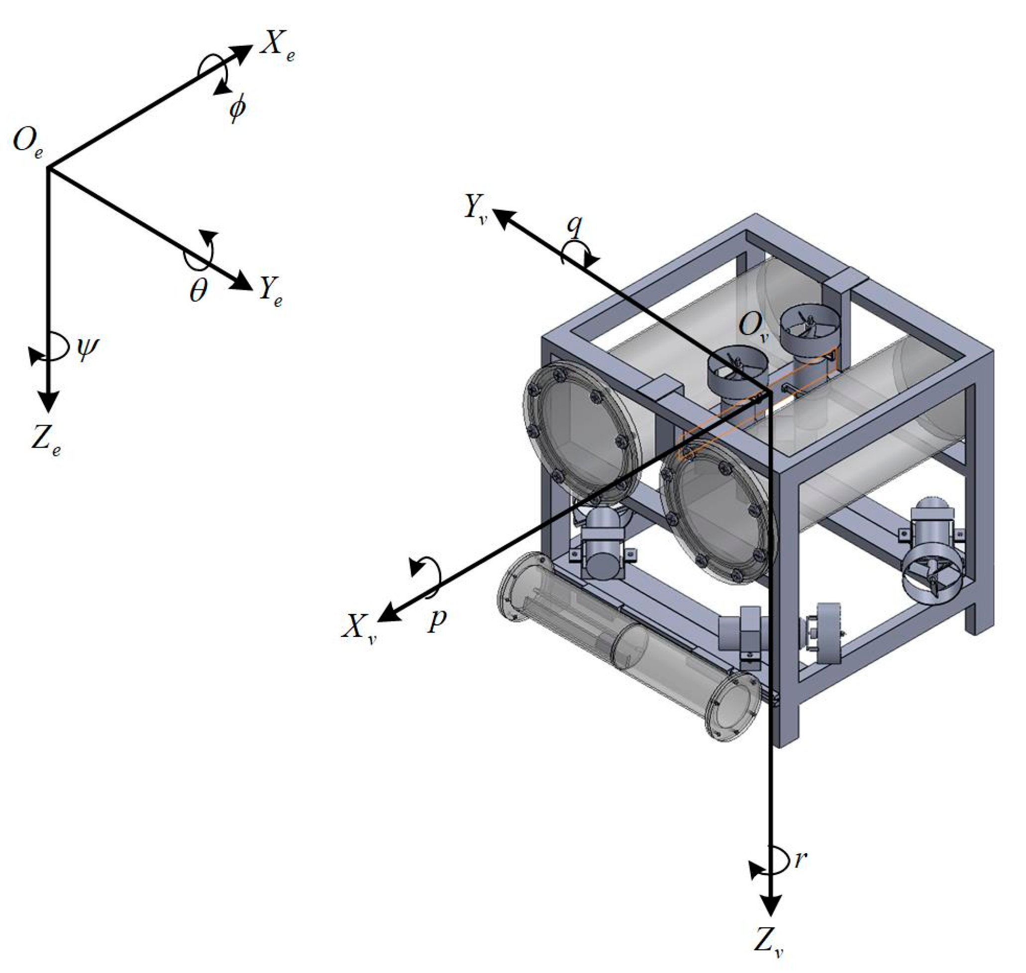
2. Motion and Dynamic Model of ROV

This section will briefly explain the ROV’s movement and dynamic model, as shown in Figure 1 including the Earth’s coordinate system and the ROV body. In the Earth coordinate system, $O_e$ is the origin point of the Earth coordinate system, $O_e{X}_e$ points to due north, $O_e{Y}_e$ points to due east, and $O_e{Z}_e$ points to the center of the Earth. In the vehicle coordinate system, $O_v$ is set as the center of the ROV, $O_v{X}_v$ points to the straight axis forward along the vehicle’s center line, $O_v{Y}_v$ points to the straight axis on the right from the vehicle’s mass center and is perpendicular to $O_v{X}_v$, and $O_v{Z}_v$ is the vehicle’s center point pointing to the straight axis vertical and downward, and is perpendicular to the $O_v{X}_v$ and $O_v{Y}_v$ planes. The motion of ROV includes the movement in the $X_v$, $Y_v$, and $Z_v$ axes of the body reference frame and the rotation around the $X_v$, $Y_v$, and $Z_v$ axes of the body reference frame. The former involves the surge ($u$), sway ($v$), and heave ($w$) velocities, and the latter involves the rolling ($p$), pitching ($q$), and yaw ($r$) angular velocities. Observing the ROV from the perspective of the Earth coordinate system, the position of the ROV center point in space can be described as $O_v\left(x_0,y_0,z_0\right)$, and the attitude angles of the ROV to the three axes of the Earth coordinate system are rolling ($\varphi$), pitching ($\theta$), and heading ($\psi$), respectively, which are called the Euler angle [23]. In this study, two thrusters [15] controlling the vertical axis synchronously were used to adjust the movement of the ROV in the direction of $O_v{Z}_v$, the pitching angle of the ROV was changed by different propulsion forces, and the movement of ROV in the $O_v{X}_v$ and $O_v{Y}_v$ planes could be changed through the control of the propulsion forces of the four horizontal thrusters.

Therefore, the movement of ROV has six degrees of freedom (surge, sway, heave, roll, pitch, and yaw), and the velocity equations for the center position of ROV about the Earth coordinate [23] can be expressed as:

$$\begin{array}{cc}{\dot{x}}_0\hfill & =u\cos \psi \cos \theta +v(\cos \psi \sin \theta \sin \varphi -\sin \psi \cos \varphi )+w(\sin \psi \sin \varphi +\cos \psi \cos \varphi \sin \theta )\hfill \\ {\dot{y}}_0\hfill & =u\sin \psi \cos \theta +v(\cos \psi \cos \varphi +\sin \varphi \sin \theta \sin \psi )+w(\sin \theta \sin \psi \cos \varphi -\cos \psi \sin \varphi )\hfill \\ {\dot{z}}_0\hfill & =-u\sin \theta +v\cos \theta \sin \varphi +w\cos \theta \cos \varphi \hfill \end{array}$$

(1)

The velocities of the Euler angle can be expressed as:

$$\begin{array}{cc}\dot{\varphi }\hfill & =p+q\sin \varphi \tan \theta +r\cos \varphi \tan \theta \hfill \\ \dot{\theta }\hfill & =q\cos \varphi -r\sin \varphi \hfill \\ \dot{\psi }\hfill & =q\frac{\sin \varphi }{\cos \theta }+r\frac{\cos \varphi }{\cos \theta }, \theta \ne \pm 90°\hfill \end{array}$$

(2)

Assuming that the ROV is a rigid body, it can be known from Newton’s law of motion that the dynamic equation of ROV can be expressed as [24,25] with the Earth coordinate system as the reference frame:

$$M_{RB}\dot{v}+C_{RB}\left(v\right)={\tau }_{RB}$$

(3)

where ${\tau }_{RB}=[\begin{array}{cc}{\tau }_{RB1}& {\tau }_{RB2}{]}^T\end{array}\in R^6$ is the external torque and control vector; $M_{RB}\in R^{6\times 6}$ is the mass matrix of the ROV; $C_{RB}\left(v\right)\in R^{6\times 6}$ is the Coriolis and centripetal matrix; $v=[\begin{array}{cc}{v}_1& v_2{]}^T\in R^6\end{array}$ is the linear velocity and angular velocity vector of ROV, namely, $v_1={[\begin{array}{ccc}u& v& w\end{array}]}^T$ and $v_2={[\begin{array}{ccc}p& q& r\end{array}]}^T$.

The external torque and control vector ${\tau }_{RB}$ include the hydrodynamic force and torque and ${\tau }_H$ includes the restoring force and torque in the damping, the inertia of the surrounding fluid and the torque $\tau$ generated by the thruster, which drives the ROV to move. Different restoring forces and torques are generated due to different speeds and acceleration of the ROV. Therefore, the nonlinear dynamic equation of ROV’s open loop can be expressed as:

$$M\dot{v}+C\left(v\right)v+D\left(v\right)v+G_f\left(\eta \right)=\tau$$

(4)

where $\eta ={[\begin{array}{cc}{\eta }_1& {\eta }_2\end{array}]}^T$ is the vector of ROV in the Earth coordinate system including position vector ${\eta }_1={[\begin{array}{ccc}{x}_0& y_0& z_0\end{array}]}^T$ and Euler angle ${\eta }_2={[\begin{array}{ccc}\varphi & \theta & \psi \end{array}]}^T$, $M=M_{RB}+M_A\in R^{6\times 6}$ is the sum of the ROV’s mass matrix and external fluid’s mass matrix, $C\left(v\right)=C_{RB}\left(v\right)+C_A\left(v\right)\in R^{6\times 6}$ is the sum of the Coriolis and centripetal matrix and the external mass force and inertia matrix, $G_f\left(\eta \right)\in R^6$ is the damping matrix caused by surrounding circulation, and $\tau \in R^6$ is the torque generated by horizontal and vertical thrusters.

3. System Design and Hardware Architecture

Figure 2 shows the system architecture diagram of the ROV, which includes two parts: onshore and underwater controls. The onshore management comprises the power source and a laptop with a human–machine interface (HMI). The onshore operator can obtain underwater information and operate the ROV through the HMI. Additionally, the operator can use the joystick to operate the ROV directly. The underwater control part is in the ROV body. There is an embedded system (NI-roboRIO) in the watertight compartment of the ROV, which is the control center of the ROV. The embedded system interlinks with the following systems: stereo machine vision system, environment monitoring system, propulsion control system, robotic arm system, and power system.

The stereo machine vision system includes two webcams to capture the image in front of the ROV. The environment monitoring system consists of an IMU sensor, a multibeam image sonar, and a pressure sensor. The IMU sensor measures the vehicle’s orientation, the sonar captures the acoustic signal in front of the ROV, and the pressure sensor fetches the current depth. The sensor data can be transmitted to the onshore laptop through the cable for monitoring and processing. The information and results can be displayed on the HMI so that the onshore operator can obtain the current state of the underwater robot.

The propulsion control system handles the output power signals of four horizontal and two vertical thrusters so that the underwater robot can achieve the designed position state through thrust. The robotic arm system can control the grabbing function of the ROV’s robotic arm through the HMI. The power system monitors the power state and dispatches the power to the subsystems.

In this study, the control center of the ROV was the roboRIO embedded controller shown in Figure 3, provided by National Instruments (NI) headquartered in Austin, TX, USA. The built-in communication interface of NI-roboRIO includes an Inter-Integrated Circuit (I²C), Serial Peripheral Interface Bus (SPI), RS-232, USB, Ethernet, the connection between pulse-width modulation (PWM) and relay, and standard sensors and actuators used by robots. The customizable control system can be developed and designed by the Laboratory Virtual Instrumentation Engineering Workbench (LabVIEW) or C programming language, with a built-in dual-core ARM Real-Time Cortex-A9 processor and Xilinx FPGA. Therefore, the HMI in this study was designed using the LabVIEW graphic control program.

The underwater thrusters of the ROV are PCD-M170E made by Rhincodon Company (Cardiff, UK), which consists of a built-in driving board and has the advantages of high efficiency, significant thrust, small volume, easy installation, and easy control. Figure 4 shows the physical appearance of the thruster, and

Table 1. Specifications of the underwater thruster.

Item	Specification	Item	Specification
Motor type	DC brushless motor	Maximum thrust	6.5 kg
Operating voltage	DC 24 V	Net weight	0.85 kg
Rated current	15 A	Control signal	PWM signal
Maximum current	16 A (instantaneous)	Signal pulse width	1000 μs (maximum value at reverse rotation) 1500 μs (start/stop) 2000 μs (maximum value at forward rotation)
Rated power	250 W
Maximum speed	4000 rpm/min
Operating depth	300 m	Signal frequency	50 Hz, constant frequency, variable duty cycle

is its specification. The speed of the thruster is controlled via PWM. The thruster has a maximum thrust of 6.5 kg and can be operated at the underwater depth of 300 m, which is easy to use and can achieve the performance required in this study.

To measure the depth position of the ROV, the P51 pressure sensor produced by Samurai Spirit Inc. (SSI, Taipei, Taiwan) was used in this study to measure the position pressure and convert it into the depth of the position. Figure 5 shows the physical appearance of the exposed pressure sensor, and Figure 6 shows the pressure sensor with the watertight enclosure. The specification of the pressure sensor is shown in

Table 2. Technical specifications of the P51 pressure sensor.

Voltage Output	0.5–4.5 V
Accuracy	±1%
Operating Pressure	15 PSI (103.42 pa)
Voltage Input	5V
Operating Temp	−40∼105 °C

. The power supply used by the pressure sensor is 5 V voltage provided by NI-roboRIO. The pressure and voltage at the current position returned by the pressure sensor are read and converted into the actual depth of work in the monitoring system through the analog input port of NI-roboRIO. After regression analysis of the measured voltage and the pressure sensor’s depth of position, the relationship between the measured voltage $v_h$ and water depth $h\left(v_h\right)$ can be expressed as follows:

$$h\left(v_h\right)=-3.8432\times v_h+1.4862$$

(5)

In Figure 7, the red curve shows the relationship between the measured voltage and water depth. The black curve shows the relationship between the estimated voltage and water depth by Equation (5). The HMI development software of the ROV used in this study was LabVIEW, a graphical program compiling platform developed by NI. HMI is an essential platform for communication between the operator and ROV. The main functions of HMI include underwater information acquisition, thruster control, and data collection. The HMI of the ROV designed in this study is shown in Figure 8, in which Area 1 offers the selection to exit the HMI, the thrusters’ startup/shutdown, mission mode selection, the change of task execution, and the display of depth value. Area 2 is the attitude gauge used to indicate the ROV’s attitude angle through the accelerometer value. The current horizontal attitude of ROV can be visually displayed. Area 3 illustrates the propulsion state of each thruster, which is rotating clockwise or counterclockwise. Area 4 is the trajectory chart of the target depth vs. the current depth. Area 5 provides an interface to operate the ROV to move forward, backward, dive down, and float up as well as the steering and translation movement. Area 6 offers the speed adjustment of each thruster, respectively.

4. The Proposed Control Method

An ROV is easily affected by buoyancy and water flow, which change the stable status of the ROV. To overcome the influence of these disturbances on ROV, we adopted the switch PI controller combined with a buck-boost converter (BBC) to follow the desired trajectory of the ROV. Figure 9 shows the flow chart of the proposed control system, among which $D_s\left(k\right)$ is the desired depth of the position of the ROV, $P_s\left(k\right)$ is the current depth of position of the ROV measured by the pressure sensor, and $e\left(k\right)=D_s\left(k\right)-P_s\left(k\right)$ is the state error of the system. The ‘switch’ block was designed to select the output $u_{st}\left(k\right)$ of an appropriate PI controller through the input state. Then, the system generates the corresponding PWM through the BBC to drive the ROV’s vertical thruster in a self-synchronous manner, so that the ROV can drive itself to the designed trajectory position. According to the designed floating-up and diving-down trajectory, the output $u_{st}\left(k\right)$ of the switch PI controller was designed as follows:

$$u_{st}\left(k\right)=\{\begin{array}{cc}{K}_{pu}e\left(k\right)+K_{iu}{\displaystyle \sum }_{i=1}^{k}e\left(i\right)& \mathrm{when} D_s\left(k\right)>D_s\left(k-1\right) \\ K_{pd}e\left(k\right)+K_{id}{\displaystyle \sum }_{i=1}^{k}e\left(i\right)& \mathrm{when} D_s\left(k\right)\le D_s\left(k-1\right)\end{array}$$

(6)

where $D_s\left(k-1\right)$ is the last design state of the system; $K_{pu}$ and $K_{iu}$ are the parameters of PI controller during ROV floating-up, while $K_{pd}$ and $K_{id}$ are the parameters of PI controller during ROV diving-down.

In this study, the Ziegler–Nichols method was used to auto-tune the PI parameters [26], and then the parameters were fine-tuned manually according to the experimental environment. After a series of tuning tasks, the underwater robot could track the sine-wave moving well in both the floating and downing states, respectively. The parameters of the floating PI controller are $K_{pu}$ = 48 and $K_{iu}$ = 0.015, respectively, while the PI parameters of the diving are $K_{pd}$ = 45 and $K_{id}$ = 0.013, respectively.

For the thrust direction and magnitude of the underwater thruster, the speed and the direction of rotation are controlled via the PWM signal. This study combined the switch PI controller with the BBC control [15]. The output $u_{st}\left(k\right)$ of the controller was converted into a PWM signal to make one thruster achieve synchronization with the other vertical thruster. The pulse-width modulation signal in one PWM cycle contains two parameters: the total cycle time $T$ and the operating time $T_{on}$, among which $T$ is fixed, that is, one pulse-width signal cycle, while the operating time is the time occupied by the high-level logic in the PWM signal. Therefore, the ratio percentage of operating time to the total time is called the duty cycle, and the duty cycle control signal is defined as follows:

$$D=\frac{T_{on}}{T}\times 100\%$$

(7)

In this study, the duty cycle of the ROV thruster control signal was realized using DC step-up and step-down converters, and its mathematical equation is defined as follows:

D(D) = D(i − 1) ± ∆D

(8)

where $\Delta D$ is the control quantity for DC step-up and step-down, which is adjusted according to the back mode or boost mode, so it is defined as follows:

$$\Delta D=\{\begin{array}{c}\eta \frac{V_s\left[i\right]-V_m}{2V_m}, \mathrm{for} \mathrm{buck} \mathrm{mode}\\ \eta \frac{V_m-V_s\left[i\right]}{2V_m}, \mathrm{for} \mathrm{boost} \mathrm{mode}\end{array}$$

(9)

where $\eta$ is the estimated efficiency; $V_s\left[i\right]$ is the voltage increment or decrement; $i=1, 2, 3,\dots , n$ is the switch times; and $V_m$ is the designed BBC output voltage. Through the varied PWM signal from HMI or the controller, we can control the clockwise or counter-clockwise rotation of the thrusters as well as their speed, and then the position and orientation of the ROV can be adjusted appropriately.

PID controller tuning is an essential but tricky problem since it is difficult to obtain the parameters in real-time in the tuning process. In [19,20,21,22], several tuning methods were proposed, and different mathematical formulas used to model the plant. From the comparison in

Table 3. Comparison of the PID control in the literature.

Literature	Control Method	Parameter Tuning Method	System Plant	Test Signal	Controller Parameters
[19]	PID control	Gershgorin bands and equivalent open-loop process	Model	Step function	Kp = 3.94 Ki = 1.77 Kp = 0.91 Tf = 0.1
[20]	PID control	Reinforcement learning algorithm	Model	Step function	Kp = 525.2879 Ki = 201.5363 Kp = 44.1397
[21]	PID control	Bacterial foraging oriented by particle swarm optimization	Model	Step function	Kp = 1.17 Ki = 0.83 Kp = 1.26
[22]	IP and PID control	Extended forced oscillation	Model	Step function	Kp = 1.43 Ti = 4.71
Proposed Method	Switch PI controller with BBC control	Ziegler–Nichols	Modeless	Step function and sinusoidal wave	Floating: Kp = 48 Ki = 0.015 Diving: Kp = 45 Ki = 0.013

, we found that the plants controlled in these studies were all mathematical models, and the controlled motions were all step functions. The controlled plant in this paper was a natural underwater vehicle, and the action was a more complex up–down sine-wave tracking than those in [19,20,21,22]. Sinusoidal wave tracking is a typical operation for controlling the vehicle to monitor and explore the underwater environment.

5. Experimental Results

To verify the efficiency of the proposed controller for tracking the ROV trajectory, we conducted some ROV experiments in the swimming pool located in the Cijin Campus of the National Kaohsiung University of Science and Technology. There is also lateral surge interference in the swimming pool. In the first experiment, the ROV dove down to 0.75 m underwater. It performed station-keeping to verify whether it could reach the desired position and maintain its depth. In the second experiment, the ROV was controlled to follow the sine-wave trajectory to ascertain the feasibility of the trajectory following under the interference of water flow.

5.1. Experiment 1: Station-Keeping Test and Evaluation

In this experiment, we let the ROV dive down to the set position and perform station-keeping to verify the ROV’s diving-down and station-keeping stability. First, we operated the ROV to dive down to 0.3 m underwater. When receiving the dive command, the controller operated the ROV to dive to 0.75 m underwater and perform station-keeping. Figure 10 shows the processes during ROV station-keeping after diving-down, and Figure 11 shows the position response curve of the ROV during diving-down, in which the blue and red lines are the set position and the diving-down trajectory, respectively. Because the ROV performs station-keeping after diving down, the control method used is a diving-sown PI controller. Figure 10a–e shows that the ROV is diving-down, and Figure 10f–h shows that the ROV is performing station-keeping at the set position. The response curve of Figure 11 demonstrates that the designed controller can operate the ROV diving down to the fixed depth smoothly. Although there is a surge, the controller can resist its interference so that the ROV can perform station-keeping at the set position stably.

5.2. Experiment 2: Trajectory Tracking Test and Evaluation

In this experiment, we performed the trajectory following work under the interference of lateral surge to verify that the designed controller could operate the ROV to the given trajectory position. In the task of tracking control, the sine-wave was used as the tracking trajectory of ROV, so the given sine-wave equation is:

$$D_s\left(k\right)=0.5+0.3sin(0.163\times k\times \Delta t)$$

(10)

The sampling time $\Delta t$ was 10 ms. The proposed switch controller selects the parameters according to the floating-up or diving-down state and drives the vertical thruster via BBC control. Figure 12 illustrates the pictures taken during trajectory tracking by the switch PI controller, Figure 13a displays the response depth curve of ROV during trajectory tracking, and Figure 13b depicts the response trajectory error. In the above illustration, the blue response trajectory curve is under the traditional PI control, and the red response trajectory curve is under the proposed switch PI control. Figure 12 shows that the ROV can heave up and down according to the desired sine-wave signal. Furthermore, the response curves of Figure 13a demonstrate that the traditional single PI controller cannot operate the ROV to float up to the given trajectory position and the ROV leads to the sinking tendency. According to the trajectory error in Figure 13b, the average difference of a traditional single PI controller was 0.1594 m, and that of the control method proposed in this study was 0.0997 m. Figure 13b also shows that the ROV with a traditional single PI controller cannot keep up with the design trajectory signal and tends to sink slowly. Figure 13c enlarges the depth curve of the proposed method in Figure 13a and shows the relation between each tracking position and the actual scene in Figure 12. The video link of the experiment is available in Supplementary Materials.

However, the proposed controller can overcome the random external interference from the trajectory error curve, which will only result in slight sine-wave vibration in the vertical error position. Then, the proposed method can effectively control the ROV’s depth position and let the ROV follow the given trajectory. This research developed a human–machine monitoring system for underwater vehicles. The operator can monitor the current state of the underwater vehicle through the human–machine interface and understand the current operation of the controller and propulsion device simultaneously. The controller is implemented through an embedded system and applied to the trajectory tracking of the underwater robot with water flow disturbance. It can be seen from Figure 13 that it is easier to achieve trajectory tracking than a single PI controller.

6. Conclusions

This paper proposed a switch PI controller combined with BBC control to resolve the necessity of station-keeping and floating-diving during the swing state trajectory tracking when an ROV is operating in the water. Generally, the propulsion force required when diving down in the water is larger than the propulsion force required when floating up, so the controller’s parameters should be different. This study proposed a switch PI controller to resolve the above problem. The experiments showed that the traditional single PI controller could not track the designed trajectory smoothly due to the influence of buoyancy. The design method of the proposed controller used the comparison of reference positions to determine whether the current underwater vehicle was tracking the ascending or descending trajectory to select the parameter compensation required by the PI controller in different states. After that, according to the current ROV depth and error signal feedback, the input control quantity required for thruster adjustment was calculated via the selected PI controller. The ROV was driven to reach the designed position through self-synchronization and varied duty cycles. The proposed method was used to overcome the influence of underwater buoyancy on ROV floating-up and diving-down to realize tracking and control. Finally, this study conducted the fixed depth of the position station-keeping test and the sine-wave variable position tracking test of ROV in the swimming pool in enclosed waters to verify the effects of the proposed and traditional PI control methods. The experimental results showed that the control method proposed in this study can track the desired trajectory better than the traditional one.

In future works, we hope that by controlling the four horizontal and two vertical thrusters simultaneously, the ROV can perform the required state and movement trajectory during underwater operations without being affected by the buoyancy and the surge in water. We also tried to adapt the PID parameter using other strategies. However, some automatic and smart methods have been proposed for the parameter tuning of PID controllers. In the future, we will consider using other approaches such as multivariable techniques for the parameters-decision task.

References

1. Kim, J.H.; Yoo, S.J. Adaptive Event-Triggered Control Strategy for Ensuring Predefined Three-Dimensional Tracking Performance of Uncertain Nonlinear Underactuated Underwater Vehicles. Mathematics 2021, 9, 137. [Google Scholar] [CrossRef]
2. Duan, K.; Fong, S.; Chen, C.L.P. Multilayer Neural Networks-Based Control of Underwater Vehicles with Uncertain Dynamics and Disturbances. Nonlinear Dyn. 2020, 100, 3555–3573. [Google Scholar] [CrossRef]
3. Yan, Z.; Wang, M.; Xu, J. Robust. Adaptive Sliding Mode Control of Underactuated Autonomous Underwater Vehicles with Uncertain Dynamics. Ocean Eng. 2019, 173, 802–809. [Google Scholar] [CrossRef]
4. Ghafoor, H.; Noh, Y. An Overview of Next-Generation Underwater Target Detection and Tracking: An Integrated Underwater Architecture. IEEE Access 2019, 7, 98841–98853. [Google Scholar] [CrossRef]
5. Sahoo, A.; Dwivedy, S.K.; Robi, P. Advancements in the Field of Autonomous Underwater Vehicle. Ocean Eng. 2019, 181, 145–160. [Google Scholar] [CrossRef]
6. Yuan, C.; Licht, S.; He, H. Formation Learning Control of Multiple Autonomous Underwater Vehicles with Heterogeneous Nonlinear Uncertain Dynamics. IEEE Trans. Cyber. 2018, 47, 2168–2267. [Google Scholar] [CrossRef] [PubMed]
7. Pinheiro, B.C.; Moreno, U.F.; Sousa, J.T.B.; Rodriguez, O.C. Kernel-function-based Models for Acoustic Localization of Underwater Vehicles. IEEE J. Ocean. Eng. 2017, 42, 603–618. [Google Scholar] [CrossRef]
8. Smallwood, D.A.; Whitcomb, L.L. Model-Based Dynamic Positioning of Underwater Robotic Vehicles: Theory and Experiment. IEEE J. Ocean. Eng. 2004, 29, 169–186. [Google Scholar] [CrossRef]
9. Hsu, L.; Costa, R.R.; Lizarralde, F.; Da Cunha, J.P.V.S. Dynamic Positioning of Remotely Operated Underwater Vehicles. IEEE Robot Autom. Mag. 2000, 7, 21–31. [Google Scholar] [CrossRef]
10. Lygouras, J.N. DC Thruster Controller Implementation with Integral Anti-wind up Compensator for Underwater ROV. J. Intell. Robot Syst. 1999, 25, 79–94. [Google Scholar] [CrossRef]
11. Koh, T.H.; Lau, M.W.S.; Seet, G.; Low, A. A Control Module Scheme for an Underactuated Underwater Robotic Vehicle. J. Intell. Robot Syst. 2006, 46, 43–58. [Google Scholar] [CrossRef]
12. Makavita, C.D.; Jayasinghe, S.G.; Nguyen, H.D.; Ranmuthugala, D. Experimental Study of a Command Governor Adaptive Depth Controller for an Unmanned Underwater Vehicle. Appl. Ocean. Res. 2019, 86, 62–71. [Google Scholar] [CrossRef]
13. Tanakitkorn1a, K.; Wilsona, P.A.; Turnocka, S.R.; Phillipsb, A.B. Depth Control for an Over-Actuated, Hover-Capable Autonomous Underwater Vehicle with Experimental Verification. Machines 2017, 41, 67–81. [Google Scholar] [CrossRef] [Green Version]
14. Zhou, H.; Liu, K.; Li, Y.; Ren, S. Dynamic Sliding Mode Control Based on Multi-model Switching Laws for the Depth Control of an Autonomous Underwater Vehicle. Int. J. Adv. Robot. Syst. 2015, 12, 142. [Google Scholar] [CrossRef] [Green Version]
15. Nag, A.; Patel, S.S.; Akbar, S.A. Fuzzy Logic Based Depth Control of an Autonomous Underwater Vehicle. In Proceedings of the 2013 International Mutli-Conference on Automation, Computing, Communication, Control and Compressed Sensing (iMac4s), Kottayam, India, 22–23 March 2013; pp. 22–23. [Google Scholar]
16. Pu, Y.C.; Kuo, C.L.; Chen, J.L.; Lin, C.H.; Yan, J.J. Bilateral Propellers Dynamic Control for an Underwater Operated Vehicle Using a Self-Synchronization Practical Tracking Controller. Ocean Eng. 2018, 150, 318–326. [Google Scholar] [CrossRef]
17. Haibao, J.; Dezhi, H.; Han, L.; Jiuzhang, H.; Wenjing, N. Time Synchronized Velocity Error for Trajectory Compression. Comput. Model. Eng. Sci. 2022, 130, 1193–1219. [Google Scholar]
18. Felipe, J.T.; Gerardo, V.G.; Carlos, D.G.; Ricardo, Z.-Y.; Mario, A.G.; Adolfo, R.L. Synchronization of Robot Manipulators Actuated by Induction Motors with Velocity Estimator. Comput. Model. Eng. Sci. 2019, 121, 609–630. [Google Scholar]
19. Thiago, A.M.E.; Pericles, R.B. Iterative Procedure for Tuning Decentralized PID Controllers. IFAC-Pap. 2015, 48, 1180–1185. [Google Scholar]
20. Miranda, M.F.; Vamvoudakis, K.G. Online optimal auto-tuning of PID controllers for tracking in a special class of linear systems. In Proceedings of the 2016 American Control Conference (ACC), Boston, MA, USA, 6–8 July 2016. [Google Scholar] [CrossRef]
21. Korani, W.M.; Dorrah, H.T.; Emara, H.M. Bacterial Foraging Oriented by Particle Swarm Optimization Strategy for PID Tuning. In Proceedings of the 10th Annual Conference Companion on Genetic and Evolutionary Computation (CIRA), Daejeon, Korea, 15–18 December 2009. [Google Scholar] [CrossRef] [Green Version]
22. Bazanella, A.S.; Pereira, L.F.A.; Parraga, A. A New Method for PID Tuning Including Plants Without Ultimate Frequency. IEEE Trans. Control Syst. Technol. 2017, 25, 637–644. [Google Scholar] [CrossRef]
23. Fossen, T.I. Handbook of Marine Craft Hydrodynamics and Motion Control; John Wiley & Sons Ltd.: Hoboken, NJ, USA, 2011. [Google Scholar]
24. Fossen, T.I. Guidance and Control of Ocean Vehicles; John Wiley & Sons Ltd.: Hoboken, NJ, USA, 1994. [Google Scholar]
25. Fossen, T.I. Marine Control Systems: Guidance, Navigation and Control of Ships, Rigs and Underwater Vehicles, Marine Cybernetics; Marine Cybernetics: Trondheim, Norway, 2002; ISBN 82-92356-00-2. [Google Scholar]
26. Ziegler, J.G.; Nichols, N.B. Optimum settings for automatic controllers. Trans. ASME 1942, 64, 759–768. [Google Scholar] [CrossRef] [Green Version]
Figure 1. Description of ROV movement using the Earth and vehicle coordinate systems.
Processes 10 02346 g001
Figure 2. System architecture diagram.
Processes 10 02346 g002
Figure 3. The physical appearance of NI-roboRIO.
Processes 10 02346 g003
Figure 4. Underwater thruster.
Processes 10 02346 g004
Figure 5. Pressure sensor.
Processes 10 02346 g005
Figure 6. Pressure sensor with the watertight enclosure.
Processes 10 02346 g006
Figure 7. Actual depth vs. estimated depth.
Processes 10 02346 g007
Figure 8. Schematic diagram of the ROV HMI.
Processes 10 02346 g008
Figure 9. System control flow chart.
Processes 10 02346 g009
Figure 10. Station-keeping experiment. (a) Start diving at the depth of −0.3 m. (b) Dive to −0.4 m. (c) Dive to −0.5 m. (d) Dive to −0.6 m. (e) Dive to −0.7 m (fh) Station keeping at −0.75 m.
Processes 10 02346 g010
Figure 11. The response depth curve of the station-keeping experiment.
Processes 10 02346 g011
Figure 12. Sine-wave heaving experiment. (a) Start diving at the depth of −0.2 m. (b) Dive-down to −0.4 m. (c) Dive-down to −0.6 m. (d) Dive-down to −0.8 m. (e) Float-up to −0.6 m. (f) Float-up to −0.4m. (g) Float-up to −0.2 m. (h) Dive-down to −3 m. (i) Dive-down to −0.45 m. (j) Dive-down to −0.65 m.
Processes 10 02346 g012
Figure 13. The system response curves of the sine-wave tracking. (a) The depth variation. (b) The error between the measured and desired depth. (c) Enlargement of (a) and the tracking positions in Figure 12.
Processes 10 02346 g013aProcesses 10 02346 g013b