A Feedforward Model Predictive Controller for Optimal Hydrocracker Operation

Abstract

Hydrocracking is an energy-intensive process, and its control system aims at stable product specifications. When the main product is diesel, the quality measure is usually 95% of the true boiling point. Constant diesel quality is hard to achieve when the feed characteristics vary and feedback control has a long response time. This work suggests a feedforward model predictive control structure for an industrial hydrocracker. A state-space model, an autoregressive exogenous model, a support vector machine regression model, and a deep neural network model are tested in this structure. The resulting reactor temperature decisions and final diesel product quality values are compared against each other and against the actual measurements. The results show the importance of the feed character measurements. Significant improvements are shown in terms of product quality as well as energy savings through decreasing the heat duty of the preheating furnace.

1. Introduction

Oil refineries attract research attention from different fronts. Solutions to refinery-wide problems, such as supply chain planning [1], production planning [2] and heat integration [3], or single unit studies for atmospheric distillation [4], and fluid catalytic cracking [5] can be found in the literature.

A hydrocracker is an essential part of modern refineries that produces light fuels from heavy crudes. These systems have a higher yield of middle distillates than fluid catalytic crackers [6]. Additionally, hydrocracking finds its place also in biorefineries to crack Fischer–Tropsch liquids [7]. In both refineries, the feed varies in terms of content concentration depending on its source, which creates a challenge to stabilize the product quality.

Due to the unknown feed and reactions that occur in hydrocracking reactors, physics-based modeling is challenging, and it is often supported by data-driven models. Physics-based models include more information about the process. However, they are challenging to set up and usually require more computational power and hence a more extended evaluation time. Therefore, data-driven models are often employed in control architectures. These models are usually derived by giving a step input to the system and measuring the output, which results in a limited operational range and unknown disturbance distortion. Using labeled data to develop models is the alternative to the step test approach. A variety of data-driven models have been tested for this process, such as product yield prediction by artificial neural networks (ANN) [8], and convolutional neural networks (CNN) [9] are also trained for similar purposes. Other efforts include reinforcement learning [10], fuzzy theory [11], and deep belief networks [12] for optimization and quality prediction.

Although different models and settings are studied in the literature, feedforward control is not tested for this application. Since the quality or the true boiling point (TBP) curve is mostly unknown for the inlet stream, feedforward information is not considered available for process optimization. Time-consuming reference methods hinder the progress. However, fast characterization methods are studied in the literature. Near-infrared (NIR) [13], mid-infrared (MIR) [14], Raman [15], and nuclear magnetic resonance (NMR) spectroscopy [16] have been tested for oil characterization with successful results. In our previous review article, the integrated use of models and soft sensors for optimization and control was discussed, and the examined literature showed that a continuous feedforward control system is achievable [17]. Therefore, the research question explored in this work is: Which data-driven models are suitable for feedforward model predictive control to ensure stable hydrocracker product quality, and what energy savings can be achieved with this control setup?

The models used for control should be able to predict the product quality using the feed quality to demonstrate the effect of feed characterization. Additionally, the reactor temperatures and the flow rates notably affect the product quality. The diesel quality indicator is usually T95, which is the temperature measured when 95% volume of the sample is distilled. A few TBP curve points are given in Figure 1. T95 is a bulk property determined by the fuel’s composition, and it is adjusted mainly by the reactor temperature, which directly affects cracking. Downstream of the reactors comes a series of distillation columns, which might be used to adjust T95. However, this option heavily affects the yield of the diesel product. Reactor temperatures serve better as manipulated variables than column temperatures for quality control.

Using a single quality indicator for diesel (T95) is enough as an output since the products are already fractionated, hence limited in their carbon number. Diesel fuel usually contains hydrocarbons in a range of 10–25 carbon species [18]. Unlike the single-point product quality indicator, the feed quality is represented using more points on the feed TBP curve for better control decisions as the feed has a greater carbon number range. The location of diesel on the TBP curve of the feed is shown in Figure 1.

While the optimization and control studies on hydrocracking cover the usefulness of different models, the effect of feedforward information needs to be reported. Four data-driven models are trained and tested in a feedforward control architecture for this study. The models use the feed TBP curve, flow rates, and reactor temperatures to predict the diesel T95. Including the feed TBP curve allows the system to behave according to the feed stream’s changing quality and achieve better quality control. The selected models are

• A first-order state-space model;
• An autoregressive exogenous (ARX) model;
• A support vector machine (SVM) regression model;
• A deep neural network (DNN) model.

These models have higher maintainability and predictability than their complex alternatives. These aspects make them good candidates to be used in an industrial setting. In addition to the capability of these models, their suitability for feedforward control is shown. The importance of feed characterization is demonstrated in terms of product quality and direct heat duty savings. Furthermore, indirect savings originating from the catalyst are discussed.

2. Materials and Methods

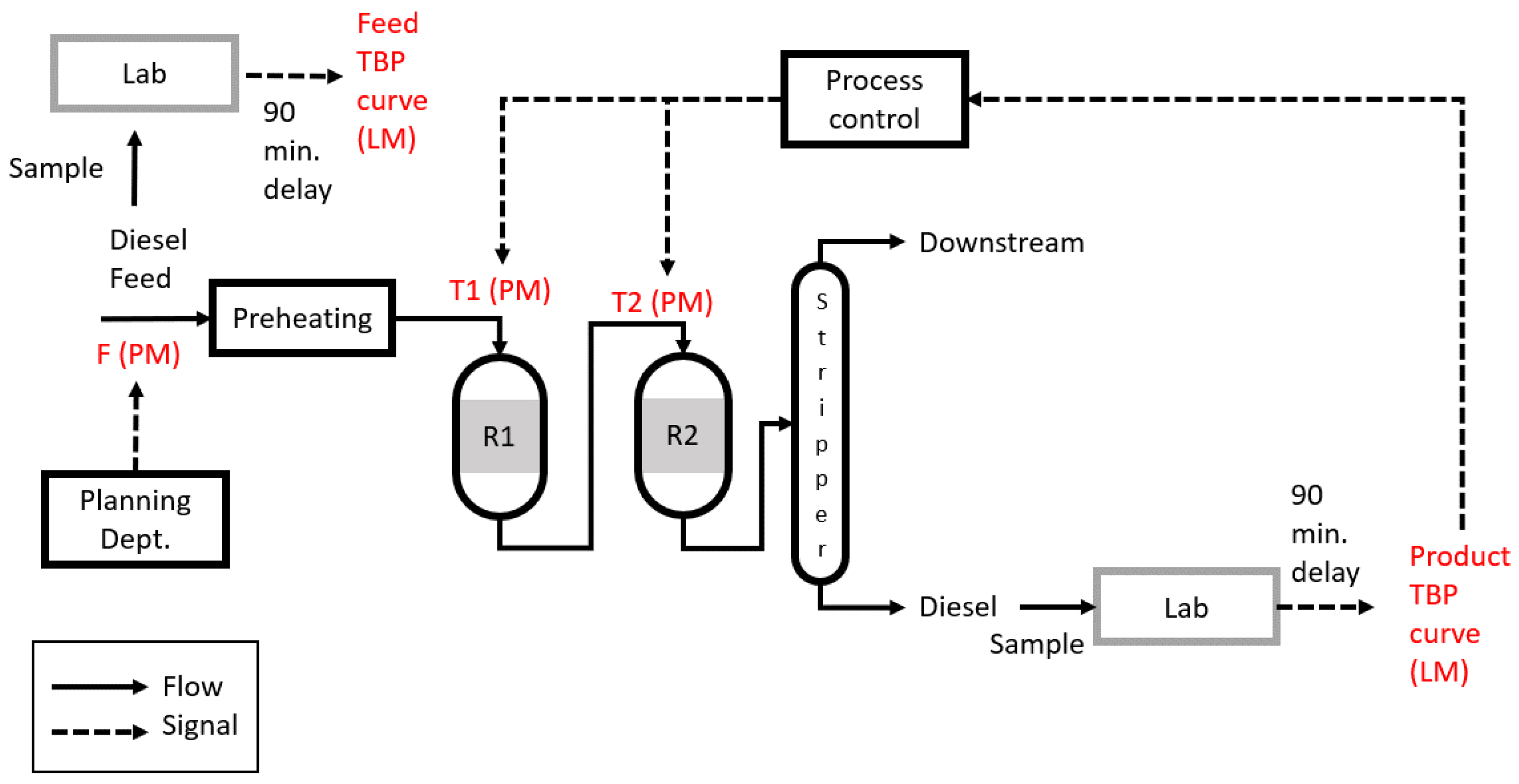
Data is collected from an industrial hydrocracker over a year. The hydrocracker unit has two reactors for cracking and distillation columns to separate the product fractions. The flowchart of the unit and its existing control structure are given in Figure 2. Locations of the lab measurements (LM) and the process measurements (PM) are marked on the figure. The planning department decides the feed flow rate (F) based on supply and demand. Reactor temperatures (T1 and T2) are adjusted with a feedback control system that has significant delays. The lab measurements include the TBP curve of the feed, diesel product, and naphtha streams. Of these products, diesel is the only one that is not further processed or blended. Therefore, the T95 of diesel is directly dependent on the temperature of this process and the feed characteristics.

Four data-driven models are trained to predict the diesel quality indicator, T95, the given reactor temperatures, and the feed TBP curve, which includes the initial boiling point, T5, T10, T30, T50, T70, T90, T95, and the final boiling point. For all four models, the same data set is used. The training data comprises 120 points and is collected over 3 months to limit the effect of catalyst degradation. The selected data is normalized and randomly assigned for training (80%) and validation (20%).

A continuous time-invariant state-space model structure is given in Equations (1) and (2), where x is the state, y is the output, and u is the input, and A, B, and C are their relevant matrices.

$$\dot{x}\left(t\right)=Ax\left(t\right)+Bu\left(t\right)$$

(1)

$$y\left(t\right)=Cx\left(t\right)$$

(2)

The general ARX structure is given in Equation (3), where A and B are polynomials of defined orders, u is the input, y is the output, n is the delay, and v is the error term. For this study, A and B are selected as fourth-order polynomials.

$$A\left(q\right)y\left(t\right)=B\left(q\right)u(t-n)+v\left(t\right)$$

(3)

While SVM is initially used for classification problems, SVM regression models are introduced by Vapnik [19] and have proven to be effective with high dimensionality and small data sets. The model is given in Equation (4) where y is the output, x is the input vector, w is the weight vector, M is the mapping function, and b is the bias vector.

$$y_i=w^{T}M\left(x\right)+b$$

(4)

DNN models are usually trained with big data and perform quite well. However, the literature includes models trained with small data sets for some applications due to data collection challenges. Material science [20], medical imaging [21], and speech–text conversion [22] studies show promising results. In the case of hydrocracking, TBP characterization limits the data collection due to the time it takes. With the reference method ASTM D86 [23], single sample analysis takes 30 min; therefore, lab measurements (LM in Figure 2) are usually limited.

The DNN structure has three fully connected hidden layers. These layers have ReLU activation functions, and the output layer is a regression layer. Adam optimizer is used for DNN training, with a maximum of 4000 epochs and a 0.013 initial learning rate. The number of nodes in all hidden layers is decided by checking all possible combinations in the 1–30 range for each layer; therefore, 27,000 networks are compared. DNN representation is given in Figure 3.

A physics-based model is used to validate the control approach. A dynamic continuous lumping structure is preferred to simulate the response, and the model equations can be found in the literature [24]. The model suggests a continuous compound distribution on the TBP curve to describe all species included in the system. A probability distribution function shows the cracking of bigger molecules into smaller ones. Mass and energy balances are integrodifferential equations due to continuity. Initialization of the compound distribution is performed by solving it as a constrained optimization problem [25]. This optimization problem is solved using sequential quadratic programming.

Since the physics-based model does not include the distillation columns’ information, the boiling point range for diesel is selected as 150 to 370 °C. The compound distribution of the relevant region is used to calculate the diesel T95 with the suggested control inputs.

Model predictive control (MPC) calculates the optimal values for manipulated variables for a selected control horizon using feedforward or feedback information, a model to predict the future behavior of the plant, and an optimization algorithm. Then, the first set of estimated values is used for the first control interval before the control horizon recedes one step for the subsequent optimization. In this case, both feedforward and feedback information is used. The sampling time and control horizon are selected according to the system dynamics (changes in feed characteristics and delays).

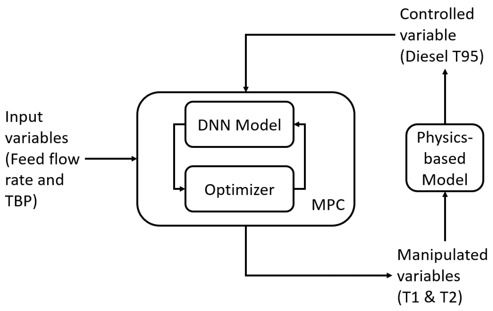
The overall system structure is given in Figure 4. By using the input variables of feed flow rate, TBP curve points, and diesel T95, the optimal reactor temperatures (T1 and T2) are calculated. These values are then fed to the physics-based model to obtain the next diesel T95. The structure is the same for all four models, and it is tested with independent test data of 200 points. Considering the measurement sensitivity, random noise is introduced on all (input and controlled) variables of a range of ±1 %.

$$\underset{T_1,T_2}{\min }\left(\sum _{t=1}^5\left(w_{sp}{(T{95}_{diesel}-T^{SP})}^2+w_R{(T_1-T_2)}^2+w_{IV}({(T_{1,t}-T_{1,t-1})}^2+{(T_{2,t}-T_{2,t-1})}^2)\right)\right)$$

(5)

The cost function used comprises three parts: setpoint tracking, penalization of temperature variation, and penalization of temperature difference between the reactors, as seen in Equation (5). A heavier importance factor is given to the setpoint from these three parts. Penalization of variation is included as the catalysts of these reactors usually do not cope well with fluctuating temperatures. Finally, the temperature difference between the two reactors is penalized for having an equal catalyst aging.

3. Results and Discussion

3.1. Data-Driven Model Training and Validation

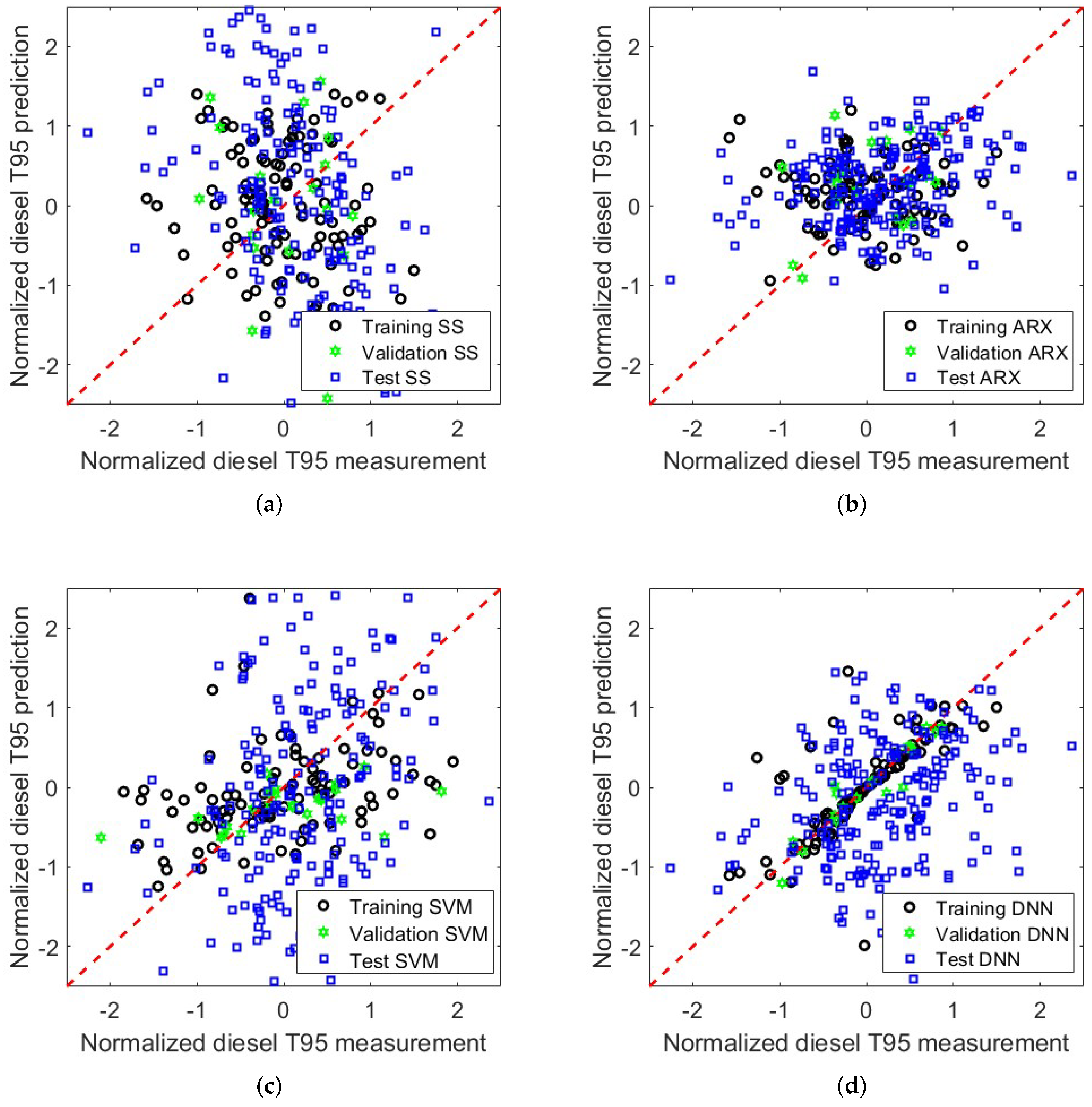
Although the system is highly nonlinear, a linear state-space model is trained for its simplicity and broad use in control applications. As expected, the accuracy of the model is not high; the root mean square error (RMSE) is 1.26 for the validation and 2.34 for the test data. The model predictions for training, validation, and test data sets are given against the lab measurements in Figure 5a.

A fourth-order ARX model is trained using the same training and validation data set. This model has a higher accuracy. The validation RMSE is 1.24 for the validation and 1.54 for the test data. ARX predictions are given in Figure 5b against the lab measurements.

An SVM regression model is trained using a linear Kernel function. The validation RMSE of this model is 0.73, and the test RMSE is 1.85. SVM predictions for the training, validation, and test set are given in Figure 5c against the lab measurements.

Finally, a DNN with three hidden layers is trained using the same data. Although often included in DNNs, drop-out and filter layers are not employed in this case due to limited available data. In total, 27,000 networks are built and compared against each other. The final network used in the rest of the study has 15–25–15 nodes in its 3 layers. The validation RMSE of the selected DNN is 0.61, and the test RMSE is 1.58. The training, validation, and test target values (measured data) are given against the prediction in Figure 5d. While the low validation RMSE indicates a good DNN model, the much higher test RMSE shows an overfitting issue, which can also be observed in Figure 5d.

3.2. Simulator Response

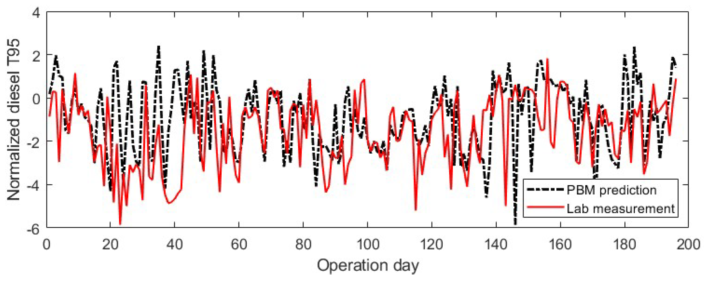
Independent control inputs are fed to the physics-based models for varying feed character, and the lab measurements are plotted against their response in Figure 6. The model gives a close enough value to the lab measurements to simulate the plant’s response to the calculated control inputs.

As stated above, the T95 of the diesel product is dependent on the reactor and distillation column temperatures. It is usually controlled by using only reactor temperatures. As cracking progresses, heavy hydrocarbons are cracked into smaller ones. There is no single reaction, as cracking can randomly happen anywhere on the carbon-carbon bounds. Some of these reactions occur more easily than others, e.g., decane cracking favors C4, C5, and C6 formation, rather than C1 and C9. However, the latter reaction does still occur [26].

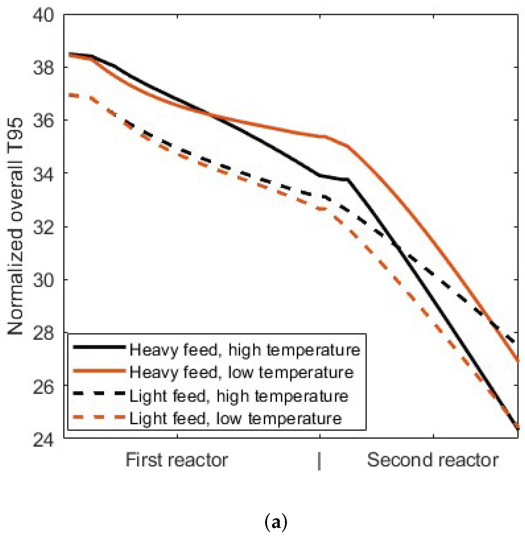
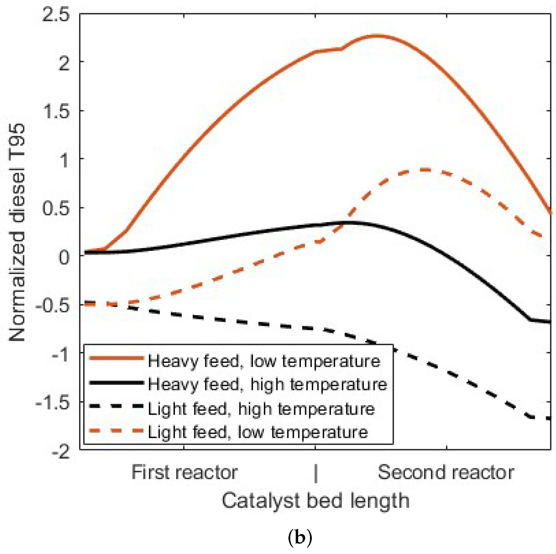
Additionally, branched and cyclic molecules have different cracking reactions due to their molecular stability. The overall T95 decreases through the catalyst bed since cracking is not an equilibrium reaction. On the other hand, the fractional T95 values (diesel and two naphtha streams for this case) might decrease or increase depending on the conditions. If cracking contributes to the heavier side more than the lighter side of one fraction or retracts the lighter side faster than the heavier side, T95 would increase.

The diesel T95 results of the physics-based model differ from those of the overall T95. A higher temperature for the same feed decreases the T95 faster than a lower temperature, as in Figure 7a. However, diesel T95 does not show the same response as the overall T95 value, given in Figure 7b. The temperature and pressure of the reactors are significant parameters, but the character of the feed is equally important to explain this behavior. A detailed reaction network analysis that includes the various cracking reactions of every single molecule would give deeper insights based on the feed content. Only very detailed structure-oriented lumping models [27], or single event microkinetic models [28] can provide a full-scale reaction prediction, and the validation is only possible via sampling at different levels of the reactor. In this study, the continuous lumping physics-based model used to obtain the diesel T95 response curve gives an approximation, which is sufficient for testing the proposed control approach. This is due to the included probabilistic equation for the cracking product, considering that every lump could be cracked into anything smaller.

3.3. Control Response

The cost function’s weight parameters used for the feedforward model predictive control (FFMPC) decision calculation are given in

Table 1. Weights and control parameters used to obtain the FFMPC response.

Parameter	Value
$w_{SP}$	6
$w_R$	1
$w_{IV}$	3
Sampling time	3
Control horizon	15

. The optimal weights might differ for each model. However, for a fair comparison, the weights are kept equal for every case in this study.

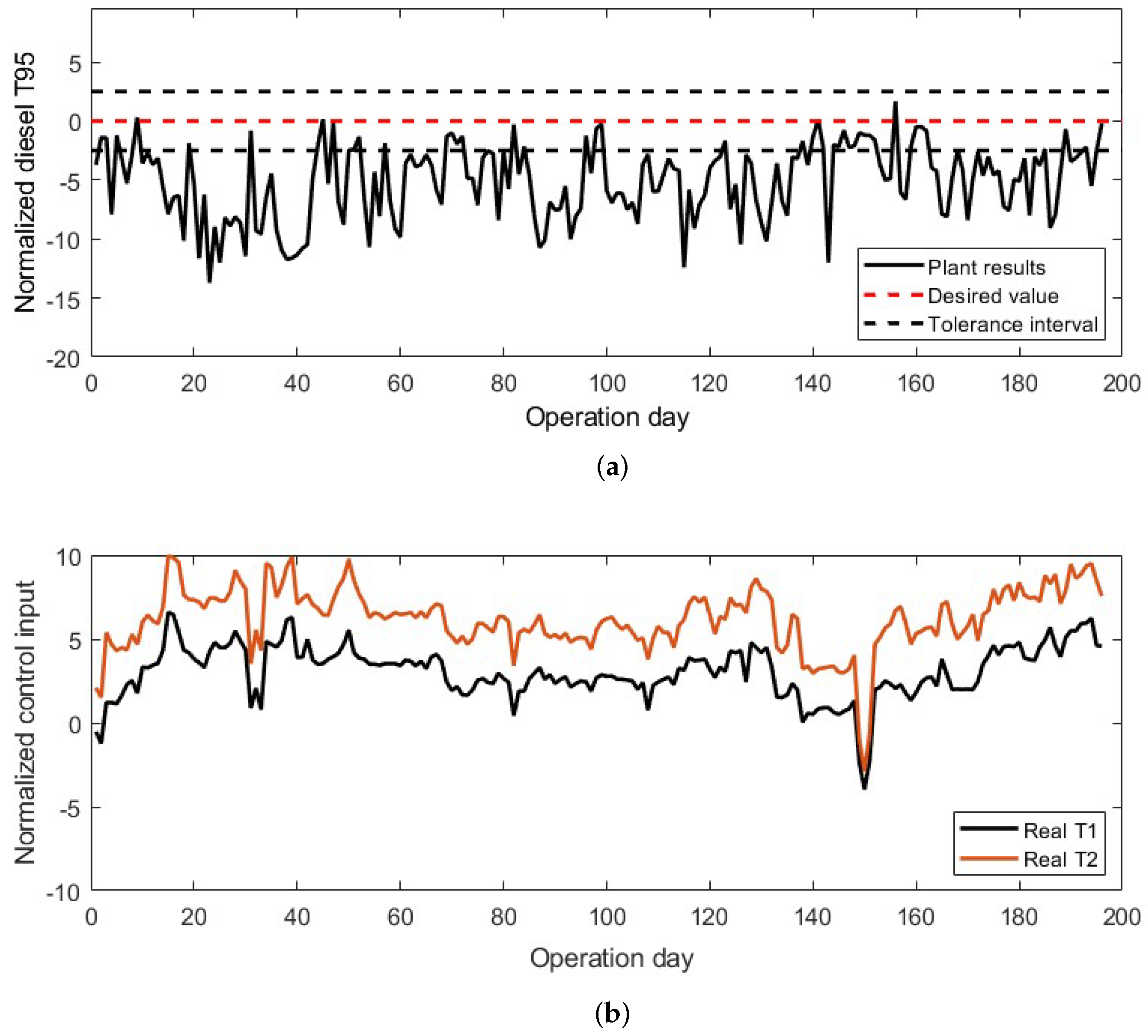
The actual diesel T95 measurements of the independent test data set are given in Figure 8a, with the desired value and tolerance interval lines. A value over the higher tolerance line is described as “off-spec” and a value below the lower bound is described as “giveaway”. These terms are used by Ref. [29] for hydrodesulfurization products and can be used for hydrocracking. While the off-spec product is of low quality, the giveaway product is of higher quality than necessary. To avoid off-spec production, the expert based control operates below the giveaway line. The product is cracked further, and the reactor temperatures are kept higher than necessary. The mean and variance of the given measurements are −4.55 and 2.60, respectively. The reactor temperatures are given in Figure 8b. The mean and variance values are 3.03 and 2.54 for the first reactor inlet temperature. The mean and variance of the second reactor’s inlet temperature are calculated as 6.19 and 3.59, respectively. The product quality measurements, reactor inlet temperatures, and their statistical information are used to assess the FFMPC improvements using four models.

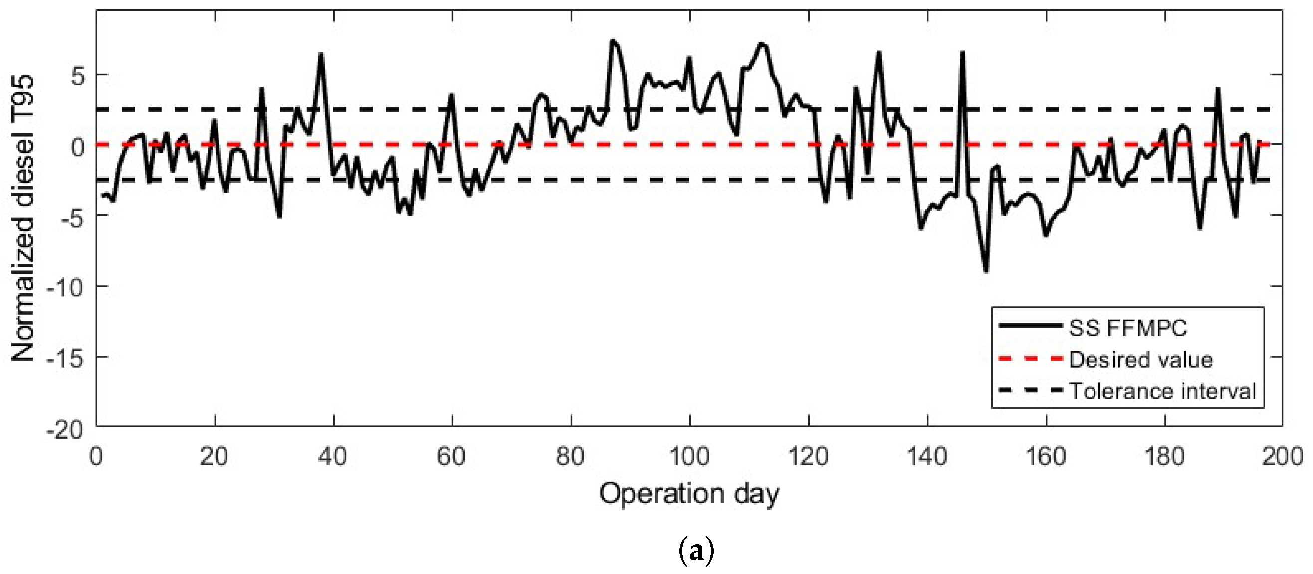
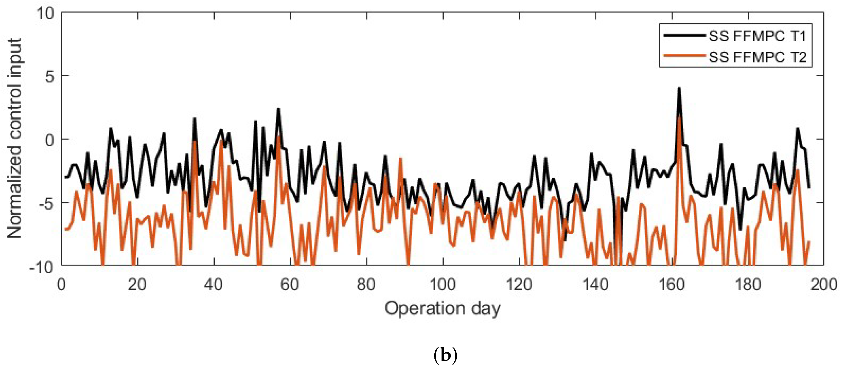
Using data-driven models and feedforward information, optimal control decisions are calculated and applied to the physics-based model for T95 estimation. The state-space model is the worst performing data-driven model of all four. When given the feedforward information, diesel T95 increases considerably compared to the existing industrial control approach. The predictions are given in Figure 9a. The mean value moves to −0.19, and the variance is 10.51 for this scenario. The reactor temperatures to reach this response are given in Figure 9b. The mean and variance values are −3.21 and 4.74 for the first reactor temperature control decisions. The second reactor’s inlet temperatures have a lower mean value of −6.73 and a higher variance of 6.50. These statistics show an improvement in their mean values. Lower mean temperatures show lower heat duty and also explain the higher diesel T95, indicating less cracking. However, all the variance values are higher than the manual feedback control. The model requires further tuning to eliminate the scattering control decisions with a higher weight of input variation.

The SVM regression model achieves a relatively stable product quality with a −0.62 mean and 1.02 variance. The diesel quality indicator results are given in Figure 10a. The mean and variance of the first reactor’s inlet temperature are calculated as 4.55 and 5.91, respectively. For the second reactor inlet temperature, these values are 4.18 and 9.66. Unlike the state space model results, the reactor temperature oscillation is smoother. While it keeps the product quality in the desired range, this model does not save energy due to increasing the mean reactor inlet temperature.

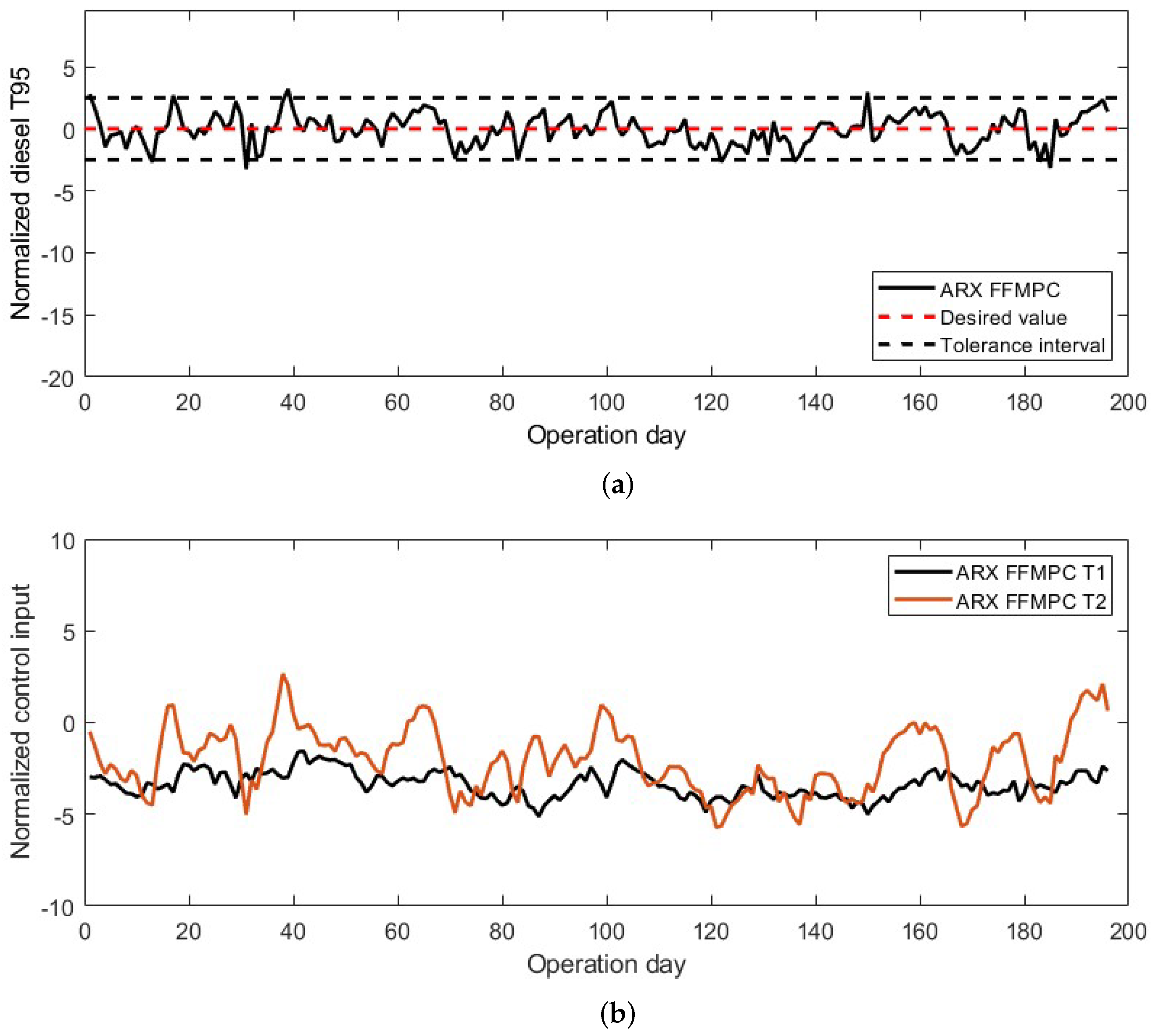
The ARX model in the control loop results in much better diesel quality, as given in Figure 11a. The mean T95 is −0.06 with a variance of 1.59 for this case. The reactor temperatures in this scenario are given in Figure 11b. The mean and variance values are −3.36, 0.50 for the first reactor’s inlet temperature and −2.07, 3.20 for the second reactor’s inlet temperature. The mean T95 is closer to the set point, and the mean temperatures are lower than those for the reference approach. Additionally, the variances are lower than those of the measured values, the state space model results, and the SVM regression results, which is due to better model accuracy.

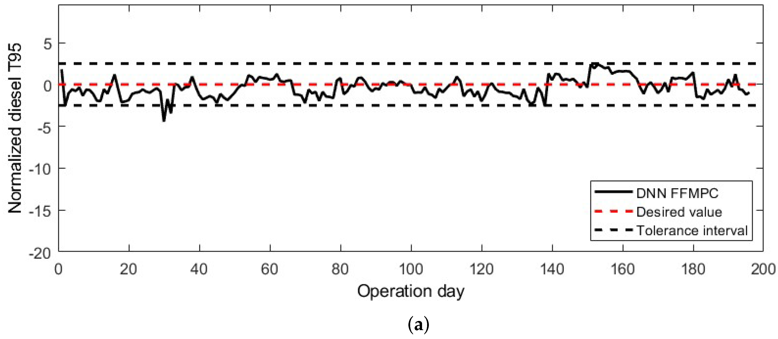
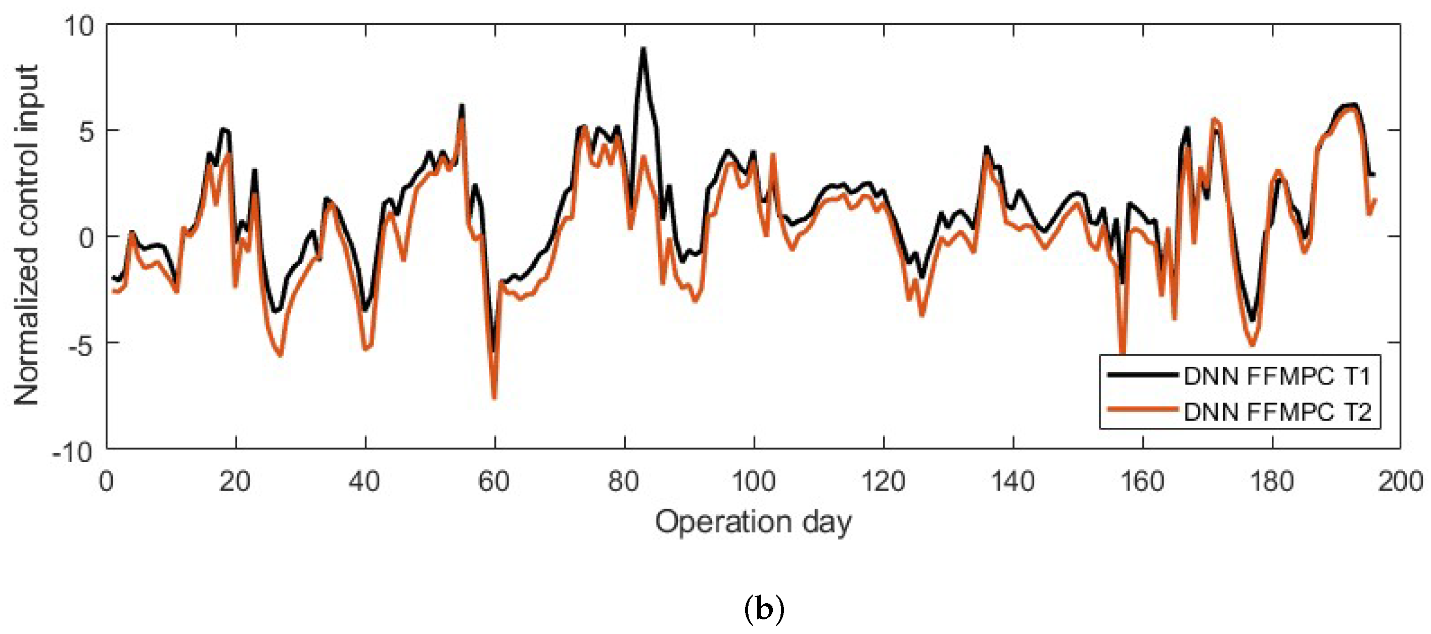
The last model tested in the same system is the DNN, and its resulting diesel T95 is given in Figure 12a. The mean and variance of these results are −0.31 and 2.66, respectively. While the mean is quite close to zero, it is not better than the ARX. The variance is similar to that of the existing system, which is higher than the ARX. The control inputs are given in Figure 12b, and the statistics show mean and variance values of 1.29 and 5.79 for the first reactor’s inlet temperature, as well as 0.33 and 6.88 for the second reactor’s inlet temperature. These still show lower heat duty than the actual system. The oscillations are not as high as the state space results but not as good as the ARX results.

Considering all the statistical information collected in

Table 2. Statistical information of the FFMPC results.

	SS Model	ARX Model	SVMR Model	DNN Model
T1 mean	−3.21	−3.36	4.18	1.29
T1 variance	4.74	0.50	9.66	5.79
T2 mean	−6.73	−2.07	4.55	0.33
T2 variance	6.50	3.20	5.91	6.88
Diesel T95 mean	−0.19	−0.06	0.62	−0.31
Diesel T95 variance	10.51	1.59	1.02	2.66

, the ARX model shows the best FFMPC performance, which is consistent with its accuracy. DNN results suffer from overfitting, which is an expected risk for a small data set. An additional contributor might be the lack of exploration in the control space. A complete space exploration is unlikely when modeling a commercial system due to the high flow rate and the possibly costly losses. A data-driven model developed under these conditions will always have some shortcomings. The overfitting issues of the DNN model can be solved by enlarging the data set since increasing the model accuracy results in improved control quality. The neural network structures give certain flexibility to the model, and for a highly nonlinear system such as hydrocracking, this might improve the data fitting capabilities. Nonetheless, these models have still proven to be useful. While evaluating a physics-based model takes around 90 s, data-driven alternatives take no longer than a second. For the iterative optimization requirement of the MPC, a detailed and accurate physics-based model might not be feasible in the short term.

Additionally, the improvement of product quality with all four models proves the importance of measuring the feed characteristics for this process. Even with the lowest accuracy linear model, the T95 is usually within the range. This range keeps the energy loss as low as possible. Part of the economic benefit of production in the tolerance interval is to prevent off-spec and giveaway product. The off-spec production cost can be attributed to energy and catalyst life through reprocessing. If the product is not marketable, it either requires reprocessing or blending with a high-quality product. Both these options add to the production cost. The giveaway product has higher quality than needed; in this case, it is lighter diesel. In the range of diesel, this product would be sold for a lower profit than naphtha streams, requiring deeper cracking and higher temperatures, which shortens the catalyst life and increases the energy consumption. Therefore, FFMPC shows energy savings and extended catalyst life. The current system uses a discrete feedback supervisory MPC for PID controllers, and the lack of feed character information is compensated for by the operator experience. After a feed change, the first reactor temperature response is observed to decide if the feed is heavy or light. The feedback information is supplied by the lab once every shift; hence, the control system is discrete.

Hydrocracking requires elevated temperatures around 30–450 °C. A preheating furnace is used to heat the feedstock from 60 °C to the process temperature that is decided by the expert or the control system. Approximately 80% of the energy input of a hydrocracker is the furnace fuel [30]. Therefore, the lower temperatures suggested by the FFMPC lower the heat load and save energy. Energy savings are calculated for each model using the difference between the actual heat duty and the required energy to reach the temperatures suggested by the FFMPC.

FFMPC using the state-space model saves 16.4% energy, which is 6.2% for the ARX and 1.4% for the DNN model. The SVM regression model does not help lower the heat duty. These values only show the lowest T1 suggested for the state-space model. However, because the product quality only sometimes stays within the desired range, these temperatures would cause other losses due to off-spec products. This energy would be a pure gain for the ARX and the DNN model solutions since the T95 is always in the range.

To realize the FFMPC, online feed and product characterization is necessary. NIR spectroscopy is a way to carry out fast TBP curve determination; it is therefore included in Figure 13. Regardless of whether NIR, NMR, or Raman spectroscopy is selected for the task, the signal flow suggested in Figure 13 would keep the product quality stable within the desired range as shown in this work, in addition to saving energy and extending the catalyst life.

4. Conclusions

In this study, four data-driven models were derived and tested in an FFMPC structure for an industrial hydrocracker. Regarding data fitting capability, the ARX model is better than the state-space, SVM regression, and DNN alternatives. Aligned with its lower RMSE value, the ARX model performs the best in the FFMPC. In addition to keeping the quality indicator in the desired range, it lowers the reactor temperature. By decreasing the heat load, the suggested FFMPC structure using the ARX model saves 6.2% of the energy required for the preheating furnace. The influence of expected savings can be appreciated considering that the furnace is the highest energy consuming equipment in this process. The temperature difference between the reactors is sufficiently low to ensure equal catalyst aging, and the lower temperatures delay degradation. The currently used expert based systems disregard the feed quality, causing product giveaway and operation at high temperatures. This work proves the importance of hydrocracker feed characterization and its use in control systems by demonstrating it with an FFMPC. The suggested structure achieves better product quality, lower furnace heat duty, and longer catalyst life. It is shown that FFMPC can ensure a lower energy-footprint hydrocracking process. Considering the petro- and bio-refineries’ total production capacity and their need for hydrocracking, this work presents the feasibility of FFMPC implementation in an industrial setup. Further work can focus on fine tuning the weight factors of the objective function for each model separately to reach their individual best performances and assess the further loss reduction potential.

References

1. Ebrahimi, S.B.; Bagheri, E. Optimizing profit and reliability using a bi-objective mathematical model for oil and gas supply chain under disruption risks. Comput. Ind. Eng. 2022, 163, 107849. [Google Scholar] [CrossRef]
2. Abdellaoui, W.; Souier, M.; Sahnoun, M.; Abdelaziz, F.B. Multi-period optimal schedule of a multi-product pipeline: A case study in Algeria. Comput. Ind. Eng. 2021, 159, 107483. [Google Scholar] [CrossRef]
3. Ryzhova, A.; Emelyanov, I.; Ziyatdinov, N.; Khalirakhmanov, Z. Optimal heat integration of large-scale cyber-physical oil refining systems. In Cyber-Physical Systems: Design and Application for Industry 4.0; Springer: Cham, Switzerland, 2021; pp. 335–345. [Google Scholar] [CrossRef]
4. Li, F.; Qian, F.; Yang, M.; Du, W.; Mahalec, V. Product tri-section based crude distillation unit model for refinery production planning and refinery optimization. AIChE J. 2021, 67, e17115. [Google Scholar] [CrossRef]
5. Chen, X.; Wu, K.; Bai, A.; Masuku, C.M.; Niederberger, J.; Liporace, F.S.; Biegler, L.T. Real-time refinery optimization with reduced-order fluidized catalytic cracker model and surrogate-based trust region filter method. Comput. Chem. Eng. 2021, 153, 107455. [Google Scholar] [CrossRef]
6. Rana, M.S.; Sámano, V.; Ancheyta, J.; Diaz, J. A review of recent advances on process technologies for upgrading of heavy oils and residua. Fuel 2007, 86, 1216–1231. [Google Scholar] [CrossRef]
7. Wijaya, K.; Nadia, A.; Dinana, A.; Pratiwi, A.F.; Tikoalu, A.D.; Wibowo, A.C. Catalytic hydrocracking of fresh and waste frying oil over Ni-and Mo-based catalysts supported on sulfated silica for biogasoline production. Catalysts 2021, 11, 1150. [Google Scholar] [CrossRef]
8. Al-Shathr, A.; Shakor, Z.M.; Majdi, H.S.; AbdulRazak, A.A.; Albayati, T.M. Comparison between Artificial Neural Network and Rigorous Mathematical Model in Simulation of Industrial Heavy Naphtha Reforming Process. Catalysts 2021, 11, 1034. [Google Scholar] [CrossRef]
9. Song, W.; Mahalec, V.; Long, J.; Yang, M.; Qian, F. Modeling the hydrocracking process with deep neural networks. Ind. Eng. Chem. Res. 2020, 59, 3077–3090. [Google Scholar] [CrossRef]
10. Oh, D.H.; Adams, D.; Vo, N.D.; Gbadago, D.Q.; Lee, C.H.; Oh, M. Actor-critic reinforcement learning to estimate the optimal operating conditions of the hydrocracking process. Comput. Chem. Eng. 2021, 149, 107280. [Google Scholar] [CrossRef]
11. Wang, Y.; Li, L.; Wang, K. An online operating performance evaluation approach using probabilistic fuzzy theory for chemical processes with uncertainties. Comput. Chem. Eng. 2021, 144, 107156. [Google Scholar] [CrossRef]
12. Yuan, X.; Rao, J.; Gu, Y.; Ye, L.; Wang, K.; Wang, Y. Online Adaptive Modeling Framework for Deep Belief Network-Based Quality Prediction in Industrial Processes. Ind. Eng. Chem. Res. 2021, 60, 15208–15218. [Google Scholar] [CrossRef]
13. Santos, F.D.; Vianna, S.G.; Cunha, P.H.; Folli, G.S.; de Paulo, E.H.; Moro, M.K.; Romão, W.; de Oliveira, E.C.; Filgueiras, P.R. Characterization of crude oils with a portable NIR spectrometer. Microchem. J. 2022, 181, 107696. [Google Scholar] [CrossRef]
14. Pasadakis, N.; Sourligas, S.; Foteinopoulos, C. Prediction of the distillation profile and cold properties of diesel fuels using mid-IR spectroscopy and neural networks. Fuel 2006, 85, 1131–1137. [Google Scholar] [CrossRef]
15. Santos, V.O., Jr.; Oliveira, F.C.; Lima, D.G.; Petry, A.C.; Garcia, E.; Suarez, P.A.; Rubim, J.C. A comparative study of diesel analysis by FTIR, FTNIR and FT-Raman spectroscopy using PLS and artificial neural network analysis. Anal. Chim. Acta 2005, 547, 188–196. [Google Scholar] [CrossRef]
16. Filgueiras, P.R.; Terra, L.A.; Castro, E.V.; Oliveira, L.M.; Dias, J.C.; Poppi, R.J. Prediction of the distillation temperatures of crude oils using 1H NMR and support vector regression with estimated confidence intervals. Talanta 2015, 142, 197–205. [Google Scholar] [CrossRef]
17. Iplik, E.; Aslanidou, I.; Kyprianidis, K. Hydrocracking: A perspective towards digitalization. Sustainability 2020, 12, 7058. [Google Scholar] [CrossRef]
18. Yuan, H.; Tsukuda, T.; Yang, Y.; Shibata, G.; Kobashi, Y.; Ogawa, H. Effects of Chemical Compositions and Cetane Number of Fischer–Tropsch Fuels on Diesel Engine Performance. Energies 2022, 15, 4047. [Google Scholar] [CrossRef]
19. Vapnik, V. The Nature of Statistical Learning Theory; Springer Science & Business Media: New York, NY, USA, 1999. [Google Scholar]
20. Feng, S.; Zhou, H.; Dong, H. Using deep neural network with small dataset to predict material defects. Mater. Des. 2019, 162, 300–310. [Google Scholar] [CrossRef]
21. Gupta, V.; Demirer, M.; Bigelow, M.; Little, K.J.; Candemir, S.; Prevedello, L.M.; White, R.D.; O’Donnell, T.P.; Wels, M.; Erdal, B.S. Performance of a deep neural network algorithm based on a small medical image dataset: Incremental impact of 3D-to-2D reformation combined with novel data augmentation, photometric conversion, or transfer learning. J. Digit. Imaging 2020, 33, 431–438. [Google Scholar] [CrossRef]
22. Sone, K.; Nakashika, T. DNN-based Speech Synthesis for Small Data Sets Considering Bidirectional Speech-Text Conversion. In Proceedings of the Interspeech 2018, Hyderabad, India, 2–6 September 2018; pp. 2519–2523. [Google Scholar]
23. ASTM-D86-19; Standard Test Method for Distillation of Petroleum Products and Liquid Fuels at Atmospheric Pressure. ASTM International: West Conshohocken, PA, USA, 2019.
24. Laxminarasimhan, C.; Verma, R.; Ramachandran, P. Continuous lumping model for simulation of hydrocracking. AIChE J. 1996, 42, 2645–2653. [Google Scholar] [CrossRef]
25. Govindhakannan, J.; Riggs, J.B. On the Construction of a Continuous Concentration- Reactivity Function for the Continuum Lumping Approach. Ind. Eng. Chem. Res. 2007, 46, 1653–1656. [Google Scholar] [CrossRef]
26. Zhang, L.; Yin, R.; Wang, J.; Li, X. Numerical Investigations on the Molecular Reaction Model for Thermal Cracking of n-Decane at Supercritical Pressures. ACS Omega 2022, 7, 22351–22362. [Google Scholar] [CrossRef] [PubMed]
27. Quann, R.J.; Jaffe, S.B. Structure-oriented lumping: Describing the chemistry of complex hydrocarbon mixtures. Ind. Eng. Chem. Res. 1992, 31, 2483–2497. [Google Scholar] [CrossRef]
28. Becker, P.J.; Serrand, N.; Celse, B.; Guillaume, D.; Dulot, H. A single events microkinetic model for hydrocracking of vacuum gas oil. Comput. Chem. Eng. 2017, 98, 70–79. [Google Scholar] [CrossRef] [Green Version]
29. Lababidi, H.; Alatiqi, I.; Ali, Y. Constrained model predictive control for a pilot hydrotreating plant. Chem. Eng. Res. Des. 2004, 82, 1293–1304. [Google Scholar] [CrossRef]
30. Boldyryev, S.; Gil, T. Debottlenecking of existing hydrocracking unit by improved heat recovery for energy and carbon dioxide savings. Energy Convers. Manag. 2021, 238, 114164. [Google Scholar] [CrossRef]
Figure 1. A representative true boiling point curve with T20, T50, T80, and T95 marks, and the location of diesel in crude oil fractions.
Processes 10 02583 g001
Figure 2. Hydrocracker unit flowchart with measurement locations and signals.
Processes 10 02583 g002
Figure 3. DNN model structure with three fully connected hidden layers.
Processes 10 02583 g003
Figure 4. FFMPC structure with a data-driven model for optimization and a physics-based model to simulate the plant response.
Processes 10 02583 g004
Figure 5. Data-driven model training and validation points against measurements. (a) State space model predictions compared against the measurements. (b) ARX model predictions compared against the measurements. (c) SVM regression model predictions compared against the measurements. (d) DNN model predictions compared against the measurements.
Processes 10 02583 g005
Figure 6. Physics-based model predictions against the lab measurements for independent control inputs.
Processes 10 02583 g006
Figure 7. Difference between overall T95 and diesel T95 behavior through the reactors. (a) Decreasing overall T95 through the catalyst bed depending on the operating temperature. (b) T95 trajectory of the diesel fraction through the reactors.
Processes 10 02583 g007aProcesses 10 02583 g007b
Figure 8. Real plant measurements of the independent test data. (a) Diesel T95 lab measurements. (b) Reactor temperatures.
Processes 10 02583 g008
Figure 9. Diesel quality and reactor temperatures estimated with the state space model. (a) Diesel T95 estimations. (b) Suggested reactor temperatures.
Processes 10 02583 g009aProcesses 10 02583 g009b
Figure 10. Diesel quality and reactor temperatures estimated with the SVM regression model. (a) Diesel T95 estimations. (b) Suggested reactor temperatures.
Processes 10 02583 g010
Figure 11. Diesel quality and reactor temperatures estimated with the ARX model. (a) Diesel T95 estimations. (b) Suggested reactor temperatures.
Processes 10 02583 g011
Figure 12. Diesel quality and reactor temperatures estimated with the DNN model. (a) Diesel T95 estimations when the DNN model is used in the control structure. (b) Suggested reactor temperatures for the DNN model.
Processes 10 02583 g012aProcesses 10 02583 g012b
Figure 13. Hydrocracker flowchart with altered signals to realize FFMPC.
Processes 10 02583 g013