Article

Queuing Models for Analyzing the Steady-State Distribution of Stochastic Inventory Systems with Random Lead Time and Impatient Customers

by
Khalid A. Alnowibet
*,
Adel F. Alrasheedi
and
Firdous S. Alqahtani
Statistics and Operations Research Department, College of Science, King Saud University, P.O. Box 2455, Riyadh 11451, Saudi Arabia
*
Author to whom correspondence should be addressed.
Processes 2022, 10(4), 624; https://doi.org/10.3390/pr10040624
Submission received: 31 December 2021 / Revised: 29 January 2022 / Accepted: 18 March 2022 / Published: 23 March 2022
(This article belongs to the Special Issue Optimization Algorithms Applied to Sustainable Production Processes)

Abstract

:
In material management, the inventory systems may have good management aspects in terms of materials; however, this negatively affects the relationship between the facility and customers. In classical inventory models, arriving demands are satisfied immediately if there is enough on-hand inventory. Traditional inventory models consider optimization problems and find the optimal policy of decision variables without computing the stationary distribution of the inventory states for random demand. Hence, a detailed analysis of inventory management systems requires a joint distribution of system stock levels and the number of requests to be investigated thoroughly. This research provides a new stochastic mathematical model for inventory systems with lead times and impatient customers under deterministic and uniform order sizes. The proposed model identifies the performance measures in a stochastic environment, analyzing the properties of the inventory system with stochastic and probabilistic parameters, and finally, validating the model’s accuracy. To analyze the system, balance equations were derived from a mathematical characterization of the underlying queuing model dependent on the Markov chain formalism. The precise performance was achieved by examining the graphical representation of the service process in a steady-state as a function of both arrival distribution and the customer patience coefficient, while it was challenging to derive an optimal curve fit in a three-dimensional space that features two input variables and a single output variable.

1. Introduction

All organizations in any sector of the economy need to manage supply chain management [1]. Effective inventory flow management in supply chains is one of the critical factors for success. Controlling the material flows from raw material suppliers to final customers is crucial. Inventory management plays a significant role in the supply chain. Currently, the strategic importance of this area is fully recognized by top management. The total investment in inventories is enormous, and the control of capital tied up in raw material, work-in-progress, and finished goods offers significant potential for improvement. Scientific methods for inventory control can give a substantial competitive advantage [2].
In practice, inventory systems cannot be decoupled from other functions such as purchasing, production, and marketing [3]. The objective of inventory control is often to balance conflicting goals. One goal is to keep stock levels down to make cash available for other purposes. On the other hand, the procurement manager may order large batches to obtain volume discounts. In the case of manufacturing, the production manager wants longer production runs to avoid setup costs that could be time-consuming or high in cost. The production manager also prefers to have a significant raw material inventory to avoid discontinuation due to a lack of raw materials [4]. The marketing department would like to have a high stock of finished goods to provide customers with a high-quality service. The challenge in managing inventory is to balance the supply of inventory with demand [5]. A company would ideally want to have enough inventory to satisfy the demands of its customers—with minimum lost sales due to inventory stock-outs.
Arriving requests are met quickly in traditional inventory models if enough product is on hand. The majority of traditional models are thought of as optimization problems in which the goal is to identify the best policy for decision variables without having to compute the stationary distribution of inventory states for random demand. Furthermore, most traditional inventory management models ignore the server’s operating time when addressing the customer’s demand. As a result, traditional inventory models solely look at the inventory level’s distribution (stationary or nonstationary).
There is, however, growing interest in the analysis of queuing systems with impatient customers [6]. Over the last decade, much attention has been paid to researching complex integrated production–inventory systems, often connected with research into integrated supply chain management. The interaction of production processes with inventory management for associated inventories is usually described using queuing networks [7] and multi-stage inventory models [8].
Some studies have derived stationary distributions by formulating long-term average cost functions used to optimize the inventory system [9,10]. In addition, the evaluation of these characteristics is usually carried out in models separated from each other. Therefore, systems are either analyzed based on inventory theory alone or queuing theory. However, a detailed analysis of inventory management systems requires a joint distribution of system stock levels and the number of requests to be investigated because inventory management systems are often closely linked to queuing systems.
This study proposes a new stochastic mathematical model for inventory systems with long lead times, and impatient customers are given order sizes that are deterministic and uniform. The preliminary model selects performance metrics in a stochastic environment, analyses inventory system aspects using stochastic and probabilistic parameters, and then, validates the model’s accuracy. Balance equations were developed from a statistical characterization of the fundamental queuing model based on the Markov chain framework to examine the process. Considering the graphical representation of the service process in a steady-state as a function of both the arrival distribution and the customer patience coefficient yielded the precise performance.
In the proposed work, we introduced the factor of variable replenishment quantity by assuming the randomness of replenishment quantity Q. This case is more realistic due to unexpected circumstances related to the supplier. Thus, the replenishment quantity is assumed to be random, although the actual order is Q. This is translated to the possibility that the supplier will not have the entire quantity Q, but he/she will supply what is variable.
We evaluated the proposed framework on a complicated model due to the randomness involved in many system factors. The process of the arrival and delivery of the order is random in most cases, and the time to deliver the order to the distributor is probably random. Furthermore, the number of goods purchased by customers could also be random. Therefore, the described model requires thorough analysis and proper distribution selection.
Our study proposes a new stochastic mathematical model for inventory systems with long lead times and impatient customers with random replenishment sizes and a uniform distribution, quickly extending to a more complex distribution.
The main focus of this research was to provide a solution for two significant queries: when to order and how much to order under the random behavior of customers and when is the best inventory position to restore the stock level. We evaluated the expected inventory that reduced the lost customers as much as possible. In addition, this research focused on the quality of service based on the customer satisfaction level.
The remaining article’s organization is as follows: Related work is given in Section 2, covering inventory models and queuing models that explore the extent of the insights used in the inventory systems. Section 3 exhibits the material and methods that include the definitions, descriptions, and parameters of the queuing models, the queuing inventory models, and the queuing model for solving the inventory model. The results and discussion are presented in Section 4, while the study is concluded in Section 5.

2. Related Work

Inventory controls are some of the critical areas of the management of an organization. There are usually no defined ways since each one is different, influenced by various features and limiting factors. The problem is related to the mathematical models, which have been developed to help formulate strategies that facilitate the achievement of optimal inventory [11]. The models are uniquely characterized, such that the optimal solutions are easily implemented to adapt to the rapidly changing situation. For instance, the conditions defining the models change daily to match the dynamism in the organization’s inventory environment [12]. At the same time, new and valuable models need to be developed with readiness for uncertainty. There are always uncertainties regardless of the control measures since it is often difficult to obtain information about some measures’ objects. Such dynamic and complex situations can be quickly addressed using systems analysis and systematic strategies to handle inventory management problems [13].

2.1. Inventory Models with Impatient Customers

An M/M/1 production system based on the (s, S) policy with impatient customers was used in [14]. The model was based on the fact that the arrival process for customers adopts a Poison distribution. The assumptions used in the model were that each production time is one unit and there are no new demands in the queue when no item is available; hence, customers for new demands were considered lost. In another model [15], the time taken by an item to move into the queue from the production system is inconsequential. It has no impact on overall performance. However, customers are described as impatient when no item is forthcoming on the production site within the model. Hence, the model focuses on maximizing inventory levels S and the production switching levels s while minimizing costs within a steady-state.
Practically, inventory problems are usually in two categories. The first category is that no circumstances will force customers to leave the system. In this case, the patience factor is infinite, even when the inventory level is at zero. The second problem is that the customer will leave once he/she becomes impatient as the inventory level goes to zero [16]. Similarly, the authors in [17] studied optimizing production under the inventory system with impatient customers. Their review described the optimal policy using the level of production base stock and admission threshold that limits the extent of accepting orders.

2.2. Queuing Models with Impatient Customers

The authors in [18] reviewed the queuing model of impatient customers based on their different dimensions. The authors first introduced anxious behaviors such as reneging, balking, and related rules before providing numerical and analytical solutions and simulations to demonstrate the model. According to the authors, impatience among customers arises from the need to experience the service. Yet, they must queue, making such customers anxious and uncomfortable while waiting for a long time [19]. The authors defined impatient behaviors in queuing using two terminologies: balking and reneging. Balking occurs when the customer decides not to join the line, while withdrawing is about joining the line, but at some point, the customer leaves without being served. Equally, some customers may renege or leave the line, but later rejoin. There are three main problems that the authors attempted to address, namely balking, reneging, and retrial. A balking customer has two decisions to make: whether to join or not join the queue when the service providers are not idle once he/she is at the service station. In this case, other researchers have proposed rules [20].
Lastly, the authors also examined retrial as part of the impatient customers in a queue [21]. Often, customers who leave a queue or renege for different reasons have the potential to rejoin the queue and repeat their particular requests at random times. Moreover, the authors in [22] identified various factors influencing customers’ impatience. These include queue length, waiting time, and busy periods. Thus, customers are likely to become impatient and either leave the queue or renege depending on the existing factors.

2.3. Queuing and Inventory Models with Different Approaches

Work on queuing models with inventory control has been vibrant amongst researchers for the past few decades. The model features the systematic arrival of customers at the facility to be served. To complete serving a customer, an item should come from the inventory. Once the customer is served, he/she immediately leaves the service point, which immediately lowers the inventory size [23]. To sustain the inventory level, there is the sourcing of items, which are supplied from outside the facility. This kind of model is called a queuing–inventory model. The inventories in this model directly influence the service, which makes the model different from traditional inventory management models [24]. Another uniqueness is that the consumption of inventories is based on serving rates rather than customer arrival rates when they queue for the service.
Queuing models with inventory problems are utilized differently depending on the existing issues and environment. They appear in different categories such as the single-server queuing with inventory, the queuing inventory system with a stochastic background, and the queuing inventory system with substitution flexibility. Altman et al. [23] proposed the single-server queuing with an inventory. According to the author, the model relies on the stationary distribution of a joint queue length and an inventory process. The inventory is continuously reviewed in this model, and new inventory management policies are established [25]. The demand for this model is based on Poisson distribution and the lead and service time’s exponential distribution. It generally adopts an M/M/1 system. While reviewing the same model, Altman et al. [23] used an M/M/1 queuing–inventory model under the (r, Q) policy with lost sales. The demand adopts a Poisson distribution with the lead and service times exponentially distributed. According to the model, all customers are lost once the stock is out.
Reference [26] proposed the queuing inventory model with a stochastic environment. The model combines queuing theory and considers lead and demand time stochastic parameters. While contributing to the same model, the authors [26] suggested that the demand process behaves according to a Poisson distribution and that production times change exponentially for a single item that makes it into the stock system. The model adopts an M/M/1/S queuing system. Equally, inventory control, in this case, adopts a multi-supplier strategy through two levels of the supply chain [27].

3. Mathematical Background

The proposed framework optimizes the system based on the decision related to the lost customers, which affects the business’s reputation, and it considers a more realistic case: the customer may decide to cancel his/her order and abandon the system. In order not to cause the loss of impatient customers, we focused on performance measures, the most important of which is when to order and how much to order under the random behavior of customers and when is the best inventory position to restore the stock level in the fastest time and service, through a calculation of the average inventory level, the average number of new orders, lost sales for new customers and impatient customers, quality of service for new customers and impatient customers, the effective arrival rate, the average number of customers in the queuing system, the average waiting time for a customer, and the waiting time in queue before the departure.

3.1. Stochastic Processes and Queuing Models

Stochastic processes are mechanisms for quantifying complex relationships in random event chains [24]. Stochastic models have a significant role in describing many aspects of natural and engineering sciences. They can also be used to examine the uncertainty inherent in biological and medical systems, resolve inconsistencies surrounding management decisions and the dynamics of psychological and social relationships, and provide new observations to assist other mathematical and statistical studies. A stochastic process is a sequence of random variables that vary over time. Examples of stochastic processes include the Poisson process, birth and death processes, continuous (discreet) Markov time chains, queuing theory, and random walk.
Based on the definition that we described for stochastic processes, this mathematically follows a family of random variables denoted by { X t , t 0 } where t is a parameter running over an appropriate index set of T. (Where possible, we can write X ( t ) instead of X t .) In a typical case, the t-index refers to discrete-time units, and the index set is T = { 0 , 1 , 2 , } . In this case, X t may represent the effects of successive coin tosses, the repeated reactions of a subject in a learning experiment, or the successive observations of certain characteristics of a population. Stochastic processes for which T = [ 0 , a u t o n o m o u s ] are especially important for applications. T mostly reflects time here, but various circumstances occur as well. For example, t can be the distance from an arbitrary origin, and  X t can count the number of defects in the interval ( 0 , t ] along the thread or the number of cars in the interval ( 0 , t ] along a highway.
Stochastic processes are described by their state-space or the range of possible values for the random variables X t , their index set T, and the dependency connection between the random variables X t . The most used classes of stochastic processes are systematically and extensively discussed for review in the following pages, along with the most valuable mathematical measurement and analysis techniques for these processes. Examples are demonstrated in the use of these processes as models. A preview of technologies from many and varied areas of interest are integral to the display.
A stochastic process X t , t 0 with possible values (state-space) T = { 0 , 1 , 2 , } is called a Markov chain. A continuous time stochastic process X t , t 0 with state-space T is called a Markov process.

3.1.1. Markov Chain

The Markov process { X t } is a stochastic process with the property that, given the value of X t , the values of X s for s > t are not affected by the values of X u for u < t . In other words, the mechanism’s likelihood of some specific future action, since its current state is well known, is not altered by additional awareness of its past attitude. A discrete-time Markov chain is a Markov process whose state-space is a finite or countable set and whose (time) index set is T = { 0 , 1 , 2 , } . In formal terms, the Markov property is that:
Pr { X n + 1 = j X 0 = i 0 , , X n 1 = i n 1 , X n = i }
= Pr { X n + 1 = j X n = i }
For all time points n and all states, i 0 , , i n 1 , i . j .
It is considered appropriate to label the state-space of the Markov chain by the nonnegative integers {0,1,2, …}, which we do, except if the inversion is explicitly stated, and it is usual to speak of X n as being in state i if X n = i .
The probability of X n + 1 being in state j given that X n is in state i is called the one-step transition probability and is denoted by P i j n . n + 1 , that is,
P i j n . n + 1 = Pr { X n + 1 = j X n = i }
The notation emphasizes that, in general, the transition probabilities are functions not only of the first and final states, but of the transition time as well. The Markov chain has stationary transition probabilities if the one-step transition probabilities are independent of the time variable n. Since most Markov chains that we shall be meeting have stationary transition probabilities, we limit our discussion to this status. Then, P i j n . n + 1 = P i j is independent of n, and  P i j is the conditional probability that the state value undergoes a transition from i to j in one trial. It is customary to arrange these numbers P i j in a matrix, in the infinite square array:
P = P 00 P 10 P 20 P i 0 P 01 P 11 P 21 P i 1 P 02 P 12 P 22 P i 2 P 03 P 13 P 23 P i 3
and we refer to P = P i j as the Markov matrix or transition probability matrix of the process.
The ith row of P, for  i = 0 , 1 , , is the probability distribution of the values of X n + 1 under the condition that X n = i . If the number of states is finite, then P is a finite square matrix whose order (the number of rows) is equal to the number of states. Clearly, the quantities P i j satisfy the conditions:
P i j 0 f o r i , j = 0 , 1 , 2 , ,
j = 0 P i j = 1 f o r i = 0 , 1 , 2 , ,
The condition merely expresses that some transition occurs at each trial (For convenience, one says that a transition has occurred even if the state remains unchanged).
A Markov process is wholly defined once its transition probability matrix and initial state X 0 (or, more generally, the probability distribution of X 0 ) are specified. We shall now prove this fact.

3.1.2. Long-Run Distribution (Stationary Distribution)

Consider an irreducible Markov chain. If the chain is positive recurrent, then the long-run proportions are the unique solution of the equations:
π j = i π i P i , j j 1
j π j = 1
Moreover, if there is no solution to the preceding linear equations, then the Markov chain is either transient or null recurrent, and all π j = 0 .

3.2. Single-Server Markovian Queuing Model with Impatient Customers

A queuing system consists of “customers” arriving at random times to some facility where they receive a service of some type and then depart. We use “customer” as a generic term. It may point, for example, to customers demanding service or a product at a time, to ships entering a port, to batches of data flowing into a computer subsystem, to broken machines awaiting repair, and so on. Queuing models are classified according to:
  • The input process, the probability distribution of the type of arrivals of customers in time;
  • The service distribution, the probability distribution of the random time to serve a customer (or group of customers in the case of a batch service);
  • The queue discipline, the number of servers, and the customer service order.
In this research, we propose an M/M/1/N queuing scheme for impatient customers. Customers arrive according to the Poisson method at a rate of λ per unit of time. The service is offered by a single server serving customers on a first-come, first-served (FCFS) basis. Service times are followed by an exponential distribution with a service rate of μ per unit of time. During the waiting time, consumers become frustrated, that is once the customer arrives at the service during the queue, the customer exits the queue. Abandon means that the abandonment process begins once the arriving customer notices one or more waiting customers in the queue. A waiting customer abandons the queue if he/she waits an exponential amount of time before quitting the service with rate α per unit of time, assuming the impatient times are independent of all others. For example, if the system is in State 3, it means that there is one customer in service and two are waiting; every customer will wait for an exponential time with rate α , and the second customer in the queue will spend another independent exponential time before leaving the system; so, the system will move from State 3 to State 2 by three streams: the first customer in the service departs the system, or the first customer in the queue abandons the system, or the second customer in the system in the queue abandons the system with rate α . The customer in the service with rate μ or the first customer in the queue abandons the system with rate α or the second customer in the queue abandons the system with rate α , so the total rate for the system from State 3 to State 2 is μ + 2 α . In general, the transition rate of the system is as follows:
λ n = λ n N 1 0 n N
μ n = μ + ( n 1 ) α n 1
The rate diagram in M/M/1/N with impatient customers is given in Figure 1.

3.2.1. Balance Equations

Based on the information above, the balance equations of M/M/1/N with impatient customers present a stationary analysis for the model described as follows:
The average rates at which the process is left (state n) = the average rates at which the process is entered (state n):
n = 0 λ P 0 = μ P 1
n = 1 λ P 1 + μ P 1 = λ P 0 + ( μ + α ) P 2 λ + μ P 1 = λ P 0 + ( μ + α ) P 2
n = 2 λ P 2 + ( μ + α ) P 2 = λ P 1 + ( μ + 2 α ) P 3 λ + μ + α P 2 = λ P 1 + ( μ + 2 α ) P 3
n = 3 λ P 3 + ( μ + 2 α ) P 3 = λ P 2 + ( μ + 3 α ) P 4 λ + μ + 2 α P 3 = λ P 2 + ( μ + 3 α ) P 4
n = N 1 λ P N 1 + μ + N 2 α P N 1 = λ P N 2 + μ + N 1 α P N
λ + μ + ( N 2 ) α P N 1 = λ P N 2 + ( μ + ( N 1 ) α ) P N
n = N ( μ + ( N 1 ) α ) P N = λ P N 1

3.2.2. Solution of the Balance Equations

Solving the balance equations of M/M/1/N from the information above is as follows:
λ P 0 = μ P 1 P 1 = λ μ P 0
λ + μ P 1 = λ P 0 + ( μ + α ) P 2 λ λ + μ λ μ μ P 0 = ( μ + α ) P 2 P 2 = λ 2 μ ( μ + α ) P 0
λ + μ + α P 2 = λ P 1 + μ + 2 α P 3 λ + μ + α λ 2 λ 2 μ + α μ μ + α P 0 = μ + 2 α P 3
P 3 = λ 3 μ ( μ + α ) ( μ + 2 α ) P 0
λ + μ + 2 α P 3 = λ P 2 + ( μ + 3 α ) P 4 λ + μ + 2 α λ 3 λ 3 ( μ + 2 α ) μ μ + α ( μ + 2 α ) P 0 = ( μ + 3 α ) P 4
P 4 = λ 4 μ ( μ + α ) ( μ + 2 α ) ( μ + 3 α ) P 0
( μ + ( N 1 ) α ) P N = λ P N 1 P N = λ ( μ + N 1 α ) P N 1
Therefore, we find that:
P 1 = λ μ P 0
P 2 = λ 2 μ ( μ + α ) P 0
P 3 = λ 3 μ ( μ + α ) ( μ + 2 α ) P 0 = λ 3 j = 1 2 μ μ + j α P 0
P 4 = λ 4 μ ( μ + α ) ( μ + 2 α ) ( μ + 3 α ) P 0 = λ 4 j = 1 3 μ μ + j α P 0
P n = λ n μ μ + α μ + 2 α ( μ + n 1 α ) P 0 = λ n j = 1 n 1 μ μ + j α P 0 n < N
Since the variables represent a steady-state distribution, then they must satisfy the assumptions of the probability as follows:
  • 0 P i 1 i = 0 , 1 , 2 , , N ;
  • n P n = 1 :
    P 0 + P 1 + P 2 + P 3 + + P N = 1 .
From Equations (11) and (12) we find that:
P 0 + λ μ P 0 + λ 2 μ ( μ + α ) P 0 + λ 3 μ ( μ + α ) ( μ + 2 α ) + + λ n μ μ + α μ + 2 α ( μ + n 1 α ) P 0 = 1
We can take P 0 as a common factor:
P 0 1 + λ μ + λ 2 μ ( μ + α ) + λ 3 j = 1 2 μ μ + j α + + λ n j = 1 n 1 μ μ + j α = 1
P 0 = 1 1 + λ μ + λ 2 μ ( μ + α ) + λ 3 j = 1 2 μ μ + j α + + λ n j = 1 n 1 μ μ + j α
P 0 = 1 1 + λ μ + i = 1 n 1 λ i + 1 j = 1 n 1 μ μ + j α
P n = P 0 ( ρ ) n n < N 0 n N
P n = 1 1 + λ μ + i = 0 n 1 λ i + 1 j = 1 n 1 μ μ + j α ( ρ ) n 0 n < N 0 o t h e r w i s e

3.2.3. Performance Measures

The average number of customers in the queuing system:
L ¯ s = n = 0 N n P n
The average number of customers waiting in line (or in the queue):
L ¯ q = L ¯ s ( 1 P 0 )
Average waiting time in the system
L ¯ s = λ W ¯ s W ¯ s = L ¯ s λ
Average waiting time in the queue
L ¯ q = λ W ¯ q W ¯ q = L ¯ q λ
The waiting time in Q before the departure
W ¯ α = 1 α

3.3. Finite Queuing–Inventory Models with Impatient Customers under a Deterministic Order Size

We propose a queuing scheme with inventory for impatient customers under a deterministic order size. In queuing during the waiting time, consumers become frustrated. Once the customer arrives at the service during the queue, the customer exits the queue. Abandonment means that the abandonment process begins once the arriving customer notices one or more waiting customers in the queue. For example, in e-commerce, the customer submits an order for some electronic services. When the order is delayed, the customer withdraws and cancels the request.
We found that when the percentage of departures increases, it affects the overall flow of customers because the customers begin to transmit the information that the procedure is long in this place. Furthermore, the real influx decreases, especially with evaluation methods such as customer evaluation for this place or measuring customer satisfaction on the Internet or social media, which makes this phenomenon spread quickly, as to whether the wait is long or the customer is impatient.
Our work took the case where the customer is actually in the system waiting for the fulfillment of his/her order, but he/she will decide to cancel the order and leave due to the long waiting time, and that is why he/she is called an impatient customer. The proposed framework focuses on those in the system and those that leave, as this type of customer has a more substantial effect on the business’s reputation. Therefore, the two models are different. In addition, we considered the case when the replenishment order quantity is either fixed or could be random following a uniform distribution.
The proposed model suggests an M/M/1/N queuing scheme with inventory for impatient customers under a deterministic order size. Customers arrive according to the Poisson process at a rate of λ customers per unit of time. The service is offered by a single server serving customers on a first-come, first-served (FCFS) basis. Service times are followed by an exponential distribution with a μ service rate per unit of time. During the waiting time, consumers become frustrated. Once the customer arrives at the service and waits in the queue, the customer may exit the queue due to the long waiting time. This means that the abandonment begins once the arriving customer finds one or more customers waiting in the queue. Any waiting customer abandons the queue if he/she waits an exponential amount of time before quitting the service with a rate of α per unit of time. It was assumed that the impatient customers are independent of all other.
Based on the description of the system, we use the following notations:
λ : average number of arrivals per unit of time.
μ : average number of customers served per unit of time.
1 ν : time to deliver new orders as a random variable that follows the exponential distribution with parameter ν .
1 α : average time for the customer to wait in a queue before abandonment.
M: the maximum quantity order.
The description mentioned above of the previously known system and assumptions can be modeled using the birth and death stochastic process with a two-dimensional state for the system (n, k). The first dimension n represents the number of customers in the system, and the second dimension k represents the number of items in inventory. Then, we can denote this birth and death process as follows:
E z = n , k : n N 0 , k 0 , , M

3.3.1. Steady-State Distribution for Queuing Inventory Models with Impatient Customers
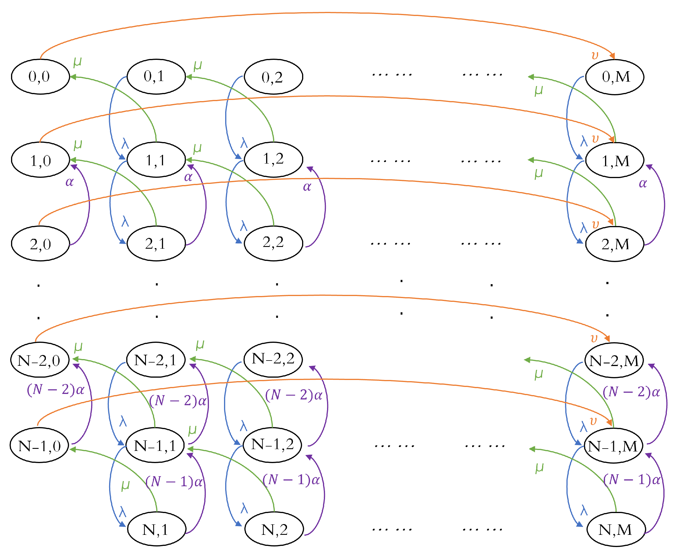
Let us assume that the order size is fixed. We have k ϵ { 0 , , M } . Then, p k = 1 for all k = M , and p k = 0 otherwise.
p k = 1 k = M 0 o t h e r w i s e

Rate Diagram

If there are customers in the system, we assume that each waiting customer is independent of the other. Each one of them has a particular waiting period. For example, if there are four customers in the system, then this means that one is in the service and three of them are waiting. Thus, we find that any of the three is qualified to leave the system after a waiting time following the exponential distribution. The rate diagram for finite queuing inventory models with impatient customers under a deterministic order size is given in Figure 2.

3.3.2. Performance Measure

We were interested in the stationary characteristics of the queuing–inventory system with impatient customers under a deterministic order size. Having determined the stationary distribution, we can compute several measures of the operating characteristics for the system explicitly. We introduced the following measures of the system performance for the stationary system:
  • Average inventory level:
Denote I ¯ as the average inventory level of the system when the system is in a steady-state. We can compute the average inventory level as follows:
I ¯ = k = 1 M k n = 0 N π n , k
When the average inventory level is very high, this means we may have to change the order quantity. If it is completely low, then this means that we will lose more customers;
  • Average number of new orders:
λ R is the average number of new orders placed by the distributor or the number of cycles per unit time when the system is in a steady-state. We can compute the average number of new orders as follows:
λ R = k = 1 M λ R k
Regarding the number of times to repeat the issuance of orders, if there are costs associated with issuing the order, then this means that we must reduce this quantity, or the maker will have to reduce it or take the necessary action and choose the appropriate M that does not make the process of issuing the order repetitive. Therefore, this will be a focus area for the decision-maker;
  • Number of cycles:
λ R k is the number of cycles when the order size is k when the system is in a steady-state. We can compute the number of cycles as follows:
λ R k = n , 0 , n , k ϵ R k π n , 0 q n , 0 , n , k = ν p k P Y = 0 ;
  • Lost sales for new customers:
L S ¯ is the expected lost sales per unit time for the new customers when the system is in the steady-state. We can compute the lost sales for new customers as follows:
L S ¯ = λ n = 0 N 1 π n , 0 + k = 1 M π N , k
Lost sales for new customers happen for two reasons. First, it may happen when the customer comes and finds a wait space, but there is not enough inventory. Second, it may happen when the customer comes and finds the waiting space is full and is unable to enter, but there is enough inventory.
Its role is to make decisions, if the quantity is high, meaning the customer’s reception space is very narrow, or the amount of orders issued is very high;
  • Lost sales for impatient customers:
L S I ¯ is the expected lost sales per unit time for the impatient customers when the system is in a steady-state. We can compute the lost sales for the impatient customers as follows:
L S I ¯ = k = 0 M n = 1 N 1 n α π ( n + 1 , k )
Lost sales for the impatient customers are another type of customer loss that differ from the previous loss, which is the length of waiting and is calculated by the number of customers who leave the system without obtaining the service or before arriving at receiving the service;
  • Lost sales per cycle for new customers:
L S ¯ c is the expected lost sales per cycle for the new customer when the system is in a steady-state. We can compute the lost sales per cycle for new customers as follows:
L S ¯ c = L S ¯ λ R ;
  • Lost sales per cycle for the impatient customer:
Denote L S I ¯ c as the expected lost sales per cycle for the impatient customers when the system is in a steady-state. We can compute the lost sales per cycle for the impatient customers as follows:
L S I ¯ c = L S I ¯ λ R ;
  • Quality of service for new customers:
β is the quality of service measure of the new customer when the system is in a steady-state. We can compute the quality of service for new customers as follows:
β = λ L S ¯ λ
The quality of service is provided to the new customers well when it is closer to one, and the quality of service is provided to the new customers badly when it is closer to zero;
  • Quality of service for impatient customers:
β I is the quality of service measure for the impatient customers when the system is in a steady-state. We can compute the quality of service for impatient customers as follows:
β I = λ L S I ¯ λ
The quality of service is provided to new customers well when it is closer to one, and the quality of service is provided to the new customers badly when it is closer to zero;
  • Effective arrival rate:
λ A is the effective arrival rate, the average number of customers entering the system per unit of time when the system is in steady-state. We can compute the effective arrival rate as follows:
λ A = λ L S ¯ ;
  • The average number of customers in the queuing system:
L ¯ s is the average number of customers in the queuing system when the system is in a steady-state. We can compute the average number of customers in the queuing system as:
L ¯ s = n = 1 N k = 1 M n π n , k + n = 1 N 1 n π n , 0 ;
  • The average number of customers waiting in line (or in the queue):
L ¯ q is the average number of customers waiting in line when the system is in a steady-state. We can compute the average number of customers waiting in line as:
E n u m b e r i n t h e s y s t e m = E n u m b e r i n q u e u e + E ( n u m b e r o f c u s t o m e r s a t t h e s e r v i c e )
E n u m b e r i n q u e u e = E n u m b e r i n t h e s y s t e m E ( n u m b e r o f c u s t o m e r s a t t h e s e r v i c e )
L ¯ q = L ¯ s P X > 0
L ¯ q = L ¯ s 1 k = 0 M π ( 0 , k ) ;
  • The average waiting time for a customer:
W ¯ q is the average waiting time for a customer when the system is in a steady-state. We can compute the average waiting time for a customer as:
W ¯ q = L ¯ q λ A
This is the average time customer waits in the queue until he/she obtains the service;
  • Sojourn time:
W ¯ s is the sojourn time when the system is in a steady-state. We can compute the sojourn time as:
W ¯ s = L ¯ s λ A
This means the time of entering the system until the departure time from the system after service is complete;
  • The waiting time in Q before the departure:
W ¯ α is the waiting time in Q before the departure when the system is in a steady-state. We can compute the waiting time in Q before the departure: empirical analysis with impatient customers under a deterministic and random order size reveals the average number of customers:
W ¯ α = 1 α .

Balance Equations

The balance equations are such that the flow process of any system situation is equal to the flow outside the system. To find the steady-state distribution (long-run distribution), we have to satisfy the stationary condition for each state in the system. This condition can be defined in general as follows:
Rate of change in state n (at time t) = rate into state n (at time t) − rate out of state n (at time t).
d d t P ( n , t ) = average rate into state n (at time t) − average rate out of state n (at time t):
E q 0 , 0 ν π 0 , 0 μ π 1 , 1 = 0
E q 0 , 1 λ π 0 , 1 μ π 1 , 2 = 0
E q 0 , 2 λ π 0 , 2 μ π 1 , 3 = 0
E q 0 , M λ π 0 , M ν π 0 , 0 = 0
E q 1 , 0 ν π 1 , 0 μ π 2 , 1 α π ( 2 , 0 ) = 0
E q 1 , 1 λ + µ π 1 , 1 λ π 0 , 1 μ π 2 , 2 α π ( 2 , 1 ) = 0
E q 1 , 2 λ + µ π 1 , 2 λ π 0 , 2 μ π 2 , 3 α π ( 2 , 2 ) = 0
E q 1 , M λ + µ π 1 , M λ π 0 , M ν π 1 , 0 α π ( 2 , M ) = 0
E q 2 , 0 ( ν + α ) π 2 , 0 μ π 3 , 1 2 α π ( 3 , 0 ) = 0
E q 2 , 1 λ + µ + α π 2 , 1 λ π 1 , 1 μ π 3 , 2 2 α π ( 3 , 1 ) = 0
E q 2 , 2 λ + µ + α π 2 , 2 λ π 1 , 2 μ π 3 , 3 2 α π ( 3 , 2 ) = 0
E q 2 , M λ + µ + α π 2 , M λ π 1 , M ν π 2 , 0 2 α π ( 3 , M ) = 0
E q 3 , 0 ( ν + 2 α ) π 3 , 0 μ π 4 , 1 3 α π ( 4 , 0 ) = 0
E q 3 , 1 λ + µ + 2 α π 3 , 1 λ π 2 , 1 μ π 4 , 2 3 α π ( 4 , 1 ) = 0
E q 3 , 2 λ + µ + 2 α π 3 , 2 λ π 2 , 2 μ π 4 , 3 3 α π ( 4 , 2 ) = 0
E q 3 , M λ + µ + 2 α π 3 , M λ π 2 , M ν π 3 , 0 3 α π ( 4 , M ) = 0
E q N 1 , 0 ( ν + ( N 2 ) α ) π N 1 , 0 μ π N , 1 = 0
E q N 1 , 1 λ + µ + ( N 2 ) α π N 1 , 1 λ π N 2 , 1 μ π N , 2 ( N 1 ) α π ( N , 1 ) = 0
E q N 1 , 2 λ + µ + ( N 2 ) α π N 1 , 2 λ π N 2 , 2 μ π N , 3 ( N 1 ) α π ( N , 2 ) = 0
E q N 1 , M λ + µ + ( N 2 ) α π N 1 , M λ π N 2 , M ν π N 1 , 0 ( N 1 ) α π ( N , M ) = 0
E q N , 1 ( µ + ( N 1 ) α ) π N , 1 λ π N 1 , 1 = 0
E q N , 2 ( µ + ( N 1 ) α ) π N , 2 λ π N 1 , 2 = 0
E q N , M ( µ + ( N 1 ) α ) π N , M λ π N 1 , M = 0

Algorithm for Solving Balance Equations

Balance equations in queuing inventory systems with impatient customers under a deterministic order size have a particular structure in each n equation and are connected to the adjacent cases or the corresponding cases. Therefore, each equation may be written within the context of the previous or subsequent variable. The algorithm we used in solving the balance equations was the linear algebra method and linear equations. These linear equations are converted into matrices due to the difficulty of solving them manually. However, if the size of the matrix is small, they can be solved manually. If the size of the matrix is large, then we solve them using linear algebra. The matrix size is the states of the two-dimensional system (n, k). Therefore, n represents the number of customers in the system, and k represents the number of items in the inventory; when the number of rows equals the number of columns, it is a square matrix. After describing the system through linear equations in the square matrix, it is called the traditional matrix A. The determinant of matrix A = 0 can easily prove that A’s determinant is equal to zero. Then, we have a vector B, which is the balance condition. Moreover, since the equations are not linear independent, we deleted the last row and replaced the whole row with the number one. It is now a matrix whose inverse we can find. Then, to find the values of π , we multiply the inverse A by the vector B.
π = A 1 × B

3.3.3. Finite Queuing–Inventory Models with Impatient Customers under a Random Order Size

Further, we propose an M/M/1/N queuing scheme with inventory for impatient customers under a random order size as the system previously described, such as the arrival and service of customers, service providers, their waiting customers, and leaving, either by the occurrence of the service or before obtaining the service, but under a random order size. Furthermore, we use the same notations, but we use the notation p k for the random order size.

Balance Equations

To find a steady-state distribution, we must satisfy the stationary condition for each state in the system. This condition can be defined in general as follows:
Rate of change in state n (at time t) = rate into state n (at time t) − rate out of state n (at time t)
d d t P ( n , t ) = average rate into state n (at time t) − average rate out of state n (at time t):
E q 0 , 0 ν π 0 , 0 μ π 1 , 1 = 0
E q 0 , 1 λ π 0 , 1 ν p 01 π 0 , 0 μ π 1 , 2 = 0
E q 0 , 2 λ π 0 , 2 ν p 02 π 0 , 0 μ π 1 , 3 = 0
E q 0 , M λ π 0 , M ν p 0 M π 0 , 0 = 0
E q 1 , 0 ν π 1 , 0 μ π 2 , 1 α π ( 2 , 0 ) = 0
E q 1 , 1 λ + µ π 1 , 1 λ π 0 , 1 μ π 2 , 2 ν p 11 π 1 , 0 α π ( 2 , 1 ) = 0
E q 1 , 2 λ + µ π 1 , 2 λ π 0 , 2 μ π 2 , 3 ν p 12 π 1 , 0 α π ( 2 , 2 ) = 0
E q 1 , M λ + µ π 1 , M λ π 0 , M ν p 1 M π 1 , 0 α π ( 2 , M ) = 0
E q 2 , 0 ( ν + α ) π 2 , 0 μ π 3 , 1 2 α π ( 3 , 0 ) = 0
E q 2 , 1 λ + µ + α π 2 , 1 λ π 1 , 1 μ π 3 , 2 ν p 21 π 2 , 0 2 α π ( 3 , 1 ) = 0
E q 2 , 2 λ + µ + α π 2 , 2 λ π 1 , 2 μ π 3 , 3 ν p 22 π 2 , 0 2 α π ( 3 , 2 ) = 0
E q 2 , M λ + µ + α π 2 , M λ π 1 , M ν p 2 M π 2 , 0 2 α π ( 3 , M ) = 0
E q 3 , 0 ( ν + 2 α ) π 3 , 0 μ π 4 , 1 3 α π ( 4 , 0 ) = 0
E q 3 , 1 λ + µ + 2 α π 3 , 1 λ π 2 , 1 μ π 4 , 2 ν p 31 π 3 , 0 3 α π ( 4 , 1 ) = 0
E q 3 , 2 λ + µ + 2 α π 3 , 2 λ π 2 , 2 μ π 4 , 3 ν p 32 π 3 , 0 3 α π ( 4 , 2 ) = 0
E q 3 , M λ + µ + 2 α π 3 , M λ π 2 , M ν p 3 M π 3 , 0 3 α π ( 4 , M ) = 0
E q N 1 , 0 ( ν + ( N 2 ) α ) π N 1 , 0 μ π N , 1 = 0
E q N 1 , 1 λ + µ + ( N 2 ) α π N 1 , 1 λ π N 2 , 1 μ π N , 2 ν p N 11 π N 1 , 0 ( N 1 ) α π ( N , 1 ) = 0
E q N 1 , 2 λ + µ + ( N 2 ) α π N 1 , 2 λ π N 2 , 2 μ π N , 3 ν p N 12 π N 1 , 0 ( N 1 ) α π ( N , 2 ) = 0
E q N 1 , M λ + µ + ( N 2 ) α π N 1 , M λ π N 2 , M ν p N 1 M π N 1 , 0 ( N 1 ) α π ( N , M ) = 0
E q N , 1 ( µ + ( N 1 ) α ) π N , 1 λ π N 1 , 1 = 0
E q N , 2 ( µ + ( N 1 ) α ) π N , 2 λ π N 1 , 2 = 0
E q N , M ( µ + ( N 1 ) α ) π N , M λ π N 1 , M = 0
We used the same algorithm to solve balance equations under a random order size through the linear algebra method.

4. Results and Discussion

This study proposed a new stochastic mathematical model for inventory systems with long lead times and impatient customers where order sizes are deterministic and uniform. The suggested model selects performance metrics in a stochastic environment, analyses inventory system aspects using stochastic and probabilistic parameters, and then, validates the model’s accuracy. Balance equations were developed from a mathematical characterization of the underlying queuing model based on the Markov chain formalism to examine the system. Examining the graphical representation of the service process in a steady-state as a function of both the arrival distribution and the customer patience coefficient yielded precise performance.
We employed several applications for each model we considered for the evaluation metrics. We observed a mechanism to deal with the balance equations to find a steady-state distribution and the best way to solve them. The algorithm we used for solving the balance equations was the linear algebra method. Moreover, we converted these linear equations into matrices using linear equations due to the difficulty of solving them manually. The general pseudocode for solving balance equations in terms of a steady-state distribution is given in Algorithm 1.
Algorithm 1 Pseudocode for solving balance equations in terms of a steady-state distribution.
1:
Define rate matrix A, and define the right-hand-side factor B.
2:
Write the balance equations in matrix form A π = B .
3:
Update matrix A by deleting the last row and using summation π i = 1 .
4:
Update the right-hand-side factor B by deleting the last row and using summation π i = 1
5:
π = A 1 × B .

4.1. Experiments with Impatient Customers under a Deterministic Order Size

Scenario: Suppose the maximal capacity of the system is equal to 10 and the maximal capacity of the inventory is equal to 10 while waiting for the product to be received during the month. Suppose that: λ = 50 , μ = 40 , ν = 45 , α = 8 . The performance measures obtained using a deterministic order size model are given in Table 1.
We observed that the average number of customers in the system equaled three, and the average number in the queue equaled two. As for the average inventory, the level equals five items, and therefore, the average number of new orders per month equaled three orders. Furthermore, the average number of a customer entering the system equaled 46, and we lost four customers per month, meaning that we lost one customer in one cycle, which means that the quality of service provided to the customers was 93%, which is considered an excellent percentage. Thus, we found that the average number of customers waiting in line equaled one day and the sojourn time until receiving the demand was equal to two days.
On the other hand, the waiting time in the queue before departure equaled four days. This indicated that the average lost sales for impatient customers per month equaled 15, and the average lost sales per customer per cycle equaled five. Therefore, the quality of service provided to impatient customers was 71%, which is considered a good percentage. Furthermore, we also observed the effect of changes in some measures on other performance measures.
If the average number of arrivals is 50, the average number of new orders delivered is 40, while the average number of abandonments for a customer is 5. The effect of changing the speed of the service on the performance measure is given in Table 2.
In order to examine the effect of the speed variation of service concerning the number of customers in a queuing system and the number of new orders under a deterministic order size, we visualize the observations using line graphs in Figure 3 and Figure 4.
From Figure 3 and Figure 4, we observed that the average number of customers in the queuing system decreased as the number of customers leaving after service increased. These phenomena were directly proportional in the case of new customers as well, as the average number of new orders increased with the number of customers leaving. The system’s efficiency increased, indicating that it provided more services and thus consumed the inventory faster. The empirical results showed an inversely proportional relation between waiting customers. They lost sales concerning the number of customers leaving, as the average number of customers waiting in line dropped and the expected lost sales for new customers went up when the number of customers leaving after service from the system gained a higher quantity.
We noticed the effect of changing the speed of service with respect to the expected lost sales for impatient customers under a deterministic order size, and it delivered a low proportion in expected lost sales and the quality of service of new customers. In terms of checking the effect of changing the order quantity on a performance measure, let us assume the maximal capacity of the system is 10, the average number of arrivals is 50, the average number of customers served is 60, the average number of new orders delivered is 40, while the average number of abandonments for a customer is 5. The effect of changing the order quantity on the performance measure is given in Table 3.
Referring to Table 3, we can see that the average inventory level grew as the number of items increased, while the average number of new orders was reduced. Similarly, the effective arrival rate was inverse and decreased when the average inventory level increased.

4.2. Experiments with Impatient Customers under a Constant Order Size

We experimented with the proposed model and derived equations under a uniform order size in several applications. We used the same linear algebra method to solve the balance equations under a constant order size. The proposed model was applied to large goods and waiting for the product to be received during the month. Consequently, if the maximal capacity of the system was two, the maximal capacity of the inventory was also two. The probability distribution with such a parameter setting with impatient customers under a uniform order size is shown in Figure 5.
Let us assume that the maximal capacity of the system is 10 and the maximal capacity of the inventory is also 10 while waiting for the product to be received during the month with λ = 50 , μ = 40 , ν = 45 , α = 8 . We encountered that the average number of customers in the system equaled three, and the average number in the queue equaled two. As for the average inventory, the level equaled four items, and therefore, the average number of new orders per month equaled five orders. Furthermore, the average number of a customers entering the system equaled 44, and we lost six customers per month, implying that we lost one customer in one cycle, which suggests that the quality of service provided to the customers was 88%. Thus, we observed that the average number of customers waiting in line equaled one day, and the sojourn time until receiving the demand was equal to two days. On the other hand, the waiting time in the queue before departure was four days. This signifies that the average lost sales for impatient customers per month equaled 14 and the average lost sales per customer per cycle equaled three. Therefore, the quality of service provided to impatient customers was 72%. In the case of the maximal capacity of the system with 20, the maximal capacity of the inventory with 30 m and λ = 60 , μ = 59 , ν = 55 , α = 5 , we found that the average number of clients in the system was three, and the average number of people waiting in line appeared as two. The level equaled ten products, so the average number of new orders per month was three when it came to the average inventory. Furthermore, the average number of consumers entering the system was 57, and we lost three clients per month, implying that we lost one customer per cycle, implying that the quality of service offered to customers was 95%, which is regarded as outstanding. As a result, we discovered that the average number of clients waiting in line was one day, and it took two days to receive the demand. The performance measures for both cases are given in Table 4.
Suppose we assumed that the maximal capacity of the system was 20 and the average number of arrivals was 60, considering the average number of served customers to be equal to 70. In that case, the average number of new orders delivered was equal to 50, while the average number of abandonments of customers equaled eight. The effect of changing the order quantity on the performance measures under a uniform order size can be seen in Table 5.
Table 5 shows that the average inventory level rose when the number of items increased. Furthermore, as the number of goods in the inventory grew, the average number of new orders fell. This was because the effective arrival rate rose as the inventory extended. We also noticed that the predicted loss of new customer sales dropped. Curves showing the effect of changing the order quantity with respect to the quality of service of new customers under a uniform order size are visualized in Figure 6.
From Figure 6, we can observe that the changing ratio reached 96% when the order quantity met 50 orders with a high quality of service for new customers. However, we can see a significant drop rate at 68% quality of service when the order proportion was too low. This indicated that when the inventory level reached a predetermined level, a replenishment order was placed to raise the inventory level to the maximum level, considering the new customers’ ratio.

5. Conclusions

Traditional inventory models analyze optimization problems without computing the stationary distribution of inventory states for random demand and finding the optimal policy of the decision variables. As a result, a complete analysis of inventory management systems necessitates a combined distribution of system stock levels and the number of requests. This research examined a new stochastic mathematical model for inventory systems with lead times and impatient customers under deterministic and uniform order sizes. Correspondingly, we analyzed the performance measures through the inventory system in a stochastic environment and explored the properties of the inventory system with stochastic and probabilistic parameters. The empirical analysis with impatient customers under deterministic and random order sizes revealed that the average number of customers in the queuing system and waiting in line dropped with the number of customers leaving after the service increased. The positive effect of changing the speed of service concerning the number of customers in a queuing system was observed. We can see that the curve of waiting customers went down as the new customers were being served. Furthermore, we found that the average number of new orders increased as the number of customers leaving after service from the system increased. As for lost sales, we encountered that the expected lost sales for impatient customers reduced as the number of customers leaving after service from the system grew, so the quality of service for impatient customers increased.
In the future, this work can be extended to finite and infinite queuing–inventory models with impatient customers using the (s, S) policy and a binomial distribution.

Author Contributions

Conceptualization, K.A.A., A.F.A. and F.S.A.; funding acquisition, K.A.A. and A.F.A.; methodology, K.A.A., A.F.A. and F.S.A.; software, K.A.A., A.F.A. and F.S.A.; writing—original draft, K.A.A., A.F.A. and F.S.A. All authors read and agreed to the published version of the manuscript.

Funding

The authors give their appreciation to King Saud University for funding this work through the Researchers Supporting Program (project number: RSP-2021/305).

Institutional Review Board Statement

Not applicable.

Informed Consent Statement

Not applicable.

Data Availability Statement

Not applicable.

Acknowledgments

The authors present their appreciation to King Saud University for funding this research through Researchers Supporting Program (Project number RSP-2021/305), King Saud University, Riyadh, Saudi Arabia.

Conflicts of Interest

The authors declare that there is no conflict of interest.

References

  1. Whitehead, T.A.; Found, P. Exploratory Research into Supply Chain Voids within Welsh Priority Business Sectors; Centre for Concurrent Enterprise, University of Nottingham Business School: Nottingham, UK, 2007. [Google Scholar]
  2. Marand, A.J.; Li, H.; Thorstenson, A. Joint inventory control and pricing in a service-inventory system. Int. J. Prod. Econ. 2019, 209, 78–91. [Google Scholar] [CrossRef]
  3. Olhager, J. The role of the customer order decoupling point in production and supply chain management. Comput. Ind. 2010, 61, 863–868. [Google Scholar] [CrossRef]
  4. Gills, B.; Thomas, J.Y.; McMurtrey, M.E.; Chen, A.N. The Challenging Landscape of Inventory Management. Am. J. Manag. 2020, 20, 39–45. [Google Scholar]
  5. Biuki, M.; Kazemi, A.; Alinezhad, A. An integrated location-routing-inventory model for sustainable design of a perishable products supply chain network. J. Clean. Prod. 2020, 260, 120842. [Google Scholar] [CrossRef]
  6. Kotb, K.; El-Ashkar, H.A. Quality control for feedback M/M/1/N queue with balking and retention of reneged customers. Filomat 2020, 34, 167–174. [Google Scholar] [CrossRef]
  7. Jain, M.; Kumar, P.; Sanga, S.S. Fuzzy Markovian modeling of machining system with imperfect coverage, spare provisioning and reboot. J. Ambient Intell. Humaniz. Comput. 2021, 12, 7935–7947. [Google Scholar] [CrossRef]
  8. Hammoudan, Z. Production and Delivery Integrated Scheduling Problems in Multi-Transporter Multi-Custumer Supply Chain with Costs Considerations. Ph.D. Thesis, Belfort-Montbéliard, Belfort, France, 2015. [Google Scholar]
  9. Helmes, K.L.; Stockbridge, R.H.; Zhu, C. Continuous inventory models of diffusion type: Long-term average cost criterion. Ann. Appl. Probab. 2017, 27, 1831–1885. [Google Scholar] [CrossRef] [Green Version]
  10. Zhao, N.; Lian, Z. A queueing-inventory system with two classes of customers. Int. J. Prod. Econ. 2011, 129, 225–231. [Google Scholar] [CrossRef]
  11. Melikov, A.; Ponomarenko, L.; Bagirova, S. Analysis of queueing-inventory systems with impatient consume customers. J. Autom. Inf. Sci. 2016, 48, 53–68. [Google Scholar] [CrossRef]
  12. Deep, K.; Jain, M.; Salhi, S. Performance Prediction and Analytics of Fuzzy, Reliability and Queuing Models: Theory and Applications; Springer: Berlin/Heidelberg, Germany, 2018. [Google Scholar]
  13. Porteus, E.L. Foundations of Stochastic Inventory Theory; Stanford University Press: Redwood City, CA, USA, 2002. [Google Scholar]
  14. Krishnamoorthy, A.; Shajin, D.; Lakshmy, B. On a queueing-inventory with reservation, cancellation, common life time and retrial. Ann. Oper. Res. 2016, 247, 365–389. [Google Scholar] [CrossRef]
  15. Melikov, A.; Ponomarenko, L. Multidimensional Queueing Models in Telecommunication Networks; Springer: Berlin/Heidelberg, Germany, 2014. [Google Scholar]
  16. Bhat, U.N. An introduction to Queueing Theory: Modeling and Analysis in Applications; Springer: Berlin/Heidelberg, Germany, 2008; Volume 36. [Google Scholar]
  17. Benjaafar, S.; Gayon, J.P.; Tepe, S. Optimal control of a production–Inventory system with customer impatience. Oper. Res. Lett. 2010, 38, 267–272. [Google Scholar] [CrossRef]
  18. Wang, K.; Li, N.; Jiang, Z. Queueing system with impatient customers: A review. In Proceedings of the 2010 IEEE International Conference on Service Operations and Logistics, and Informatics, Qingdao, China, 15–17 July 2010; pp. 82–87. [Google Scholar]
  19. Al-Begain, K.; Heindl, A.; Telek, M. Analytical and Stochastic Modeling Techniques and Applications. In Proceedings of the 15th International Conference, ASMTA 2008, Nicosia, Cyprus, 4–6 June 2008; Springer: Berlin/Heidelberg, Germany, 2008; Volume 5055. [Google Scholar]
  20. Artalejo, J.R.; Gómez-Corral, A. Retrial Queueing Systems: A Computational Approach; Springer: Berlin/Heidelberg, Germany, 2008. [Google Scholar]
  21. Yue, W.; Takahashi, Y.; Takagi, H. Advances in Queueing Theory and Network Applications; Springer: Berlin/Heidelberg, Germany, 2009. [Google Scholar]
  22. Baccelli, F.; Bremaud, P. Elements of Queueing Theory: Palm Martingale Calculus and Stochastic Recurrences; Springer Science & Business Media: Berlin/Heidelberg, Germany, 2013; Volume 26. [Google Scholar]
  23. Altman, E.; Yechiali, U. Analysis of Customers’ Impatience in Queues with Server Vacations. Queueing Syst. 2006, 52, 261–279. [Google Scholar] [CrossRef] [Green Version]
  24. Heyman, D.P.; Sobel, M.J. Stochastic Models in Operations Research: Stochastic Optimization; Courier Corporation: North Chelmsford, MA, USA, 2004; Volume 2. [Google Scholar]
  25. Choi, T.M. Handbook of EOQ Inventory Problems: Stochastic and Deterministic Models and Applications; Springer: Berlin/Heidelberg, Germany, 2013; Volume 197. [Google Scholar]
  26. Allen, A. Statistics and Queuing Theory with Computer Science Applications; Academic Press: Cambridge, MA, USA, 1990; Volume 2. [Google Scholar]
  27. Tulsian, P. Quantitative techniques: Theory and Problems; Pearson Education: Delhi, India, 2006. [Google Scholar]
Figure 1. Rate diagram for a single-server queuing model with impatient customers.
Processes 10 00624 g001
Figure 2. Rate diagram for finite queuing inventory models with impatient customers under a deterministic order size.
Processes 10 00624 g002
Figure 3. Effect of changing the speed of service with respect to the number of customers in a queuing system under a deterministic order size.
Processes 10 00624 g003
Figure 4. Effect of changing the speed of service with respect to the number of new orders under a deterministic order size.
Processes 10 00624 g004
Figure 5. The probabilities with the maximal capacity of the system are equal to 5, and the maximal capacity of the inventory is equal to 4 using impatient customers under a uniform order size.
Processes 10 00624 g005
Figure 6. Effect of changing the order quantity with respect to the quality of service of new customers under a uniform order size.
Processes 10 00624 g006
Table 1. The performance measures obtained using a deterministic order size model.
L ¯ s 2.672 cust
I ¯ 5.118 unit
λ R 3.174 new order
L S ¯ 3.676 lost cust
L S ¯ c 1.158 lost cust per cycle
β 0.926 ≈ 93%
λ A 46.324 cust entering
W ¯ s 0.058 ≈ 2 days
W ¯ α 0.125 ≈ 4 days
L S I ¯ 14.581 impatient cust
L S I ¯ c 4.593 impatient cust per cycle
β I 0.708 ≈ 71%
L ¯ q 1.823
W ¯ q 0.039 ≈ 1 day
Table 2. The effect of changing the speed of the service on the performance measure when the maximal capacity of the system and the maximal capacity of the inventory is 10 with impatient customers under a deterministic order size.
N = 10, M = 10, λ = 50, ν = 40, α = 5
μ 25303540455055606570
L ¯ s 5.304.623.983.412.932.522.181.901.681.49
I ¯ 5.185.135.095.055.025.004.984.974.964.95
λ R 2.302.683.003.273.493.663.803.914.004.07
L S ¯ 5.384.944.754.704.734.814.894.975.055.12
L S ¯ c 2.341.851.581.441.361.311.291.271.261.26
β 0.890.900.910.910.910.900.900.900.900.90
λ A 44.6245.0645.2545.3045.2745.2045.1145.0344.9544.88
W ¯ s 0.120.100.090.080.060.060.050.040.040.03
L S I ¯ 21.6018.3115.2812.6310.408.587.105.924.984.22
L S I ¯ c 9.396.855.103.872.982.341.871.521.251.04
β I 0.570.630.690.750.790.830.860.880.900.92
L ¯ q 4.323.663.062.532.081.721.421.181.000.84
W ¯ q 0.100.080.070.060.050.040.030.030.020.02
Table 3. Effect of changing the order quantity on the performance measure when the maximal capacity of the system is ten and the maximal capacity of the inventory is variable with impatient customers under a deterministic order size.
N = 10, λ = 50, μ = 60, ν = 40, α = 5
M2510152025303540
L ¯ s 1.671.831.901.931.941.951.961.961.96
I ¯ 0.982.474.977.479.9712.4814.9817.4819.98
λ R 13.877.093.912.702.061.671.401.211.06
L S ¯ 17.378.934.973.472.672.181.851.611.43
L S ¯ c 1.251.261.271.281.301.311.321.331.35
β 0.650.820.900.930.950.960.960.970.97
λ A 32.6341.0745.0346.5347.3347.8248.1548.3948.57
W ¯ s 0.050.040.040.040.040.040.040.040.04
L S I ¯ 4.895.625.926.046.106.136.166.186.19
L S I ¯ c 0.350.791.522.242.963.684.405.125.84
β I 0.900.890.880.880.880.880.880.880.88
L ¯ q 0.981.121.181.211.221.231.231.241.24
W ¯ q 0.030.030.030.030.030.030.030.030.03
Table 4. The performance measures obtained using a constant order size model.
λ = 50 , μ = 40 , ν = 45 , α = 8 λ = 60 , μ = 59 , ν = 55 , α = 5
L ¯ s 2.583 cust2.751 cust
I ¯ 3.520 unit10.096 unit
λ R 5.437 new order2.924 new order
L S ¯ 6.171 lost cust3.256 lost cust
L S ¯ c 1.135 lost cust per cycle1.091 lost cust per cycle
β 0.877 ≈ 88%0.946 ≈ 95%
λ A 43.829 cust entering56.744 cust entering
W ¯ s 0.0589 ≈ 2 days0.052 ≈ 2 days
W ¯ α 0.125 ≈ 4 days0.2 ≈ 6 days
L S I ¯ 13.928 impatient cust10.483 impatient cust
L S I ¯ c 2.562 impatient cust per cycle3.512 impatient cust per cycle
β I 0.721 ≈ 72%0.825 ≈ 83%
L ¯ q 1.7412.097
W ¯ q 0.0397 ≈ 1 day0.037 ≈ 1 day
Table 5. Effect of changing the order quantity on the performance measures considering that the maximal capacity of the system is 10 and the maximal capacity of the inventory is variable with impatient customers under a uniform order size.
N = 10, λ u p = 50, μ u p = 60, ν u p = 40, α u p = 5
M2510152025303540
L ¯ s 1.601.751.841.881.911.921.931.941.94
I ¯ 0.781.723.355.006.658.329.9811.6413.31
λ R 16.5110.526.564.773.743.082.622.282.01
L S ¯ 20.6613.208.276.044.773.943.372.942.61
L S ¯ c 1.251.261.261.271.271.281.291.291.30
β 0.590.740.830.880.900.920.930.940.95
λ A 29.3436.8041.7343.9645.2346.0646.6347.0647.39
W ¯ s 0.050.050.040.040.040.040.040.040.04
L S I ¯ 4.585.265.665.845.946.006.046.086.10
L S I ¯ c 0.280.500.861.231.591.952.312.673.03
β I 0.910.890.890.880.880.880.880.880.88
L ¯ q 0.921.051.131.171.191.201.211.221.22
W ¯ q 0.030.030.030.030.030.030.030.030.03
Publisher’s Note: MDPI stays neutral with regard to jurisdictional claims in published maps and institutional affiliations.

