1. Introduction
These studies were carried out on the basis of experimental data obtained in the course of experiments with an adjustable asynchronous traction electric drive of a shuttle car (
Figure 1) for the mining industry in the years 2010–2012.
The technical level and competitiveness of engineering products is largely determined by the controllability, reliability and level of energy consumption (efficiency) of their actuators. According to the set of technical characteristics, at present, electromechanical drives equipped with asynchronous motors with a squirrel-cage rotor have a clear advantage. This is especially important for special equipment operating in polluted, explosive conditions of mines when working in a confined space. One of these means is a shuttle car (
Figure 1), which transports heavy ore and rock through the mine, moving from the tunneling machine to the conveyor. Its main mechanism is a traction electric drive. The traction electric drive (
Figure 2a) must ensure the movement of a loaded wagon with a total weight of 30–35 tons at different travel speeds from 0.5 to 2.5 m/s. The car moves along the track with a length of 100 to 400 m with angles from −12 to +12 degrees. The traction drive power is 180 kW.
About the features of the traction electric motor, it should be noted that it has significant active resistances of the stator and rotor, significant critical slip (up to 80%) and comparable electromagnetic inertia of the rotor and stator-time constants (about 100 ms). Starting
and critical torques
are very significant in relation to the nominal (2–2.5 times). The electric motor was designed specifically for the shuttle car (
Figure 1), but not for frequency regulation; therefore, during its development, we were guided by the principles of “regulated” asynchronous electric motors, i.e., with soft mechanical characteristics (curve 1 on
Figure 2b) and displacement of the reactive section into the zone of negative velocities. This paper does not aim to compare the advantages of such motors with respect to more modern solutions adopted for variable speed drives, i.e., based on the motor with high rigidity and low starting torques (curve 2 on
Figure 2b). The purpose of this work is the analysis of processes in a nonlinear electromechanical system.
Asynchronous electric drives with frequency control are the most widespread example of nonlinear electromechanical systems in modern industry, transport and energy. The traditional methods for describing processes in these electric drives are Park’s vector equations [
1,
2,
3], vector diagrams and equivalent circuits, mechanical characteristics [
4,
5,
6], etc. At variable (adjustable) frequencies of the stator voltage, they have significant errors. The representations of nonlinear mathematical operations of torque formation by vector relations, which are fundamentally valid only for constant frequencies of the stator voltage, for processes with fast dynamics of load torques do not allow even a qualitative analysis of the reasons for the features of the processes [
6,
7,
8]. These features include the variability of the self-oscillation parameters of the effective values of the stator currents of induction motors with load changes, which is analyzed in this article.
2. Formulation of the Problem
Experiments were carried out to optimize the stator currents of an induction motor. To do this, at different speeds, races were made on three sections 50–100 m long with ascents and descents at different stator voltages for different parameters: track 1 (
Figure 3), track 2 (
Figure 4) and track 3 (
Figure 5,
Figure 6 and
Figure 7).
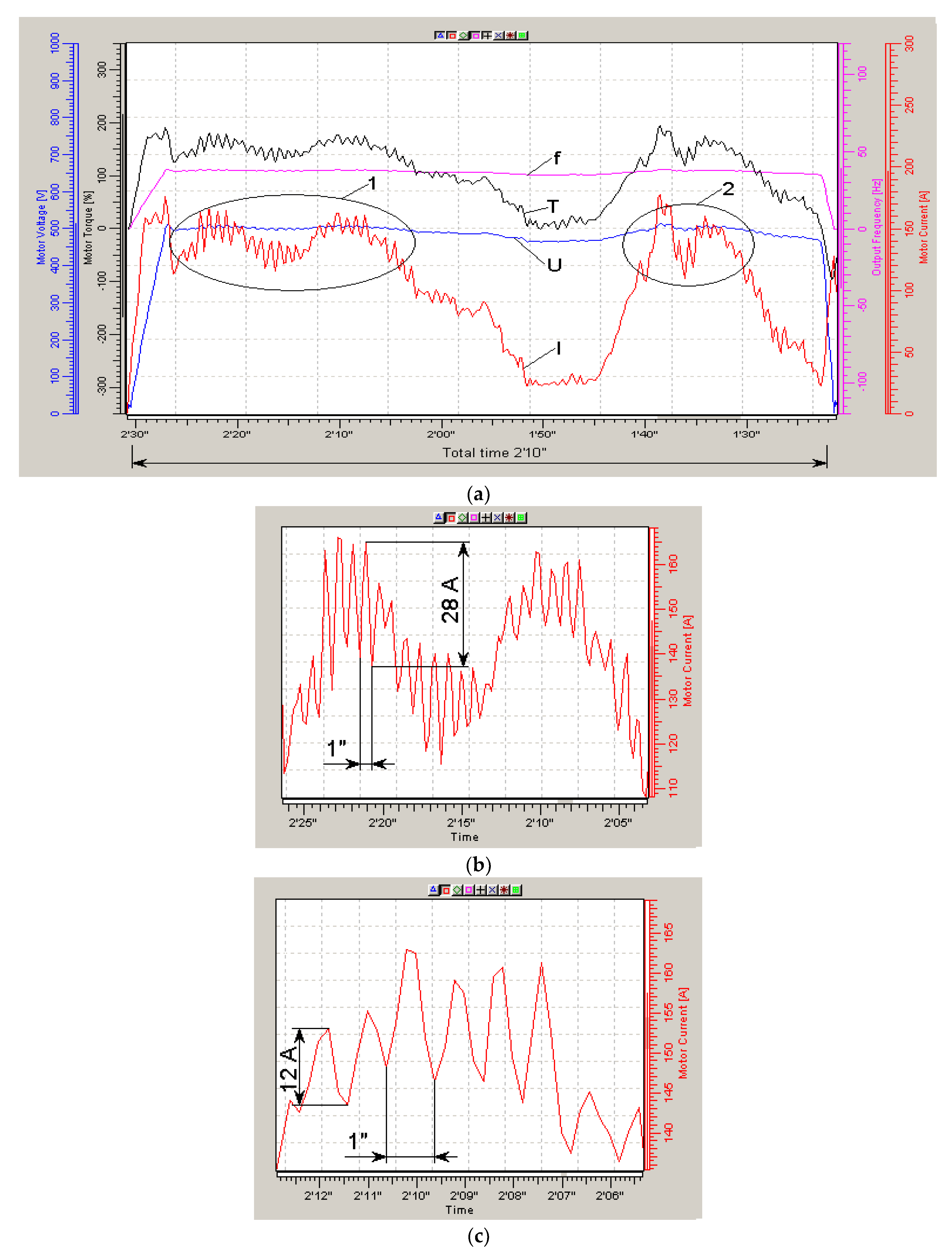
In this case, the stator current (I), frequency (f) and stator voltage amplitude (U) of the electric motor were recorded. The main parameter was the U/f ratio (determining the main magnetic flux in the motor and further denoted by the conventional units “Fl”) for three speeds: low (0.5 m/s), medium (1.5 m/s) and high (2.5 m/s).
The timing diagrams were taken by the NCDrive program, while the effective values of the stator currents (red diagram) were obtained by direct measurements and the torque diagram (black diagram) was obtained by the calculation method in the Vacon converter. Therefore, the analysis will be carried out mainly according to the diagrams of the effective values of the stator current of the traction motor (I).
By changing the parameters of the stator voltage, it was possible to reduce the average effective values of the stator currents by 20%, increasing the carrying capacity by the same 20% (
Figure 3a,b) when driving at an average speed. At the same time, it turned out that with an increase in the main magnetic flux on track 1, the stator currents decrease at high loads and increase at low loads when driving along track 2 (
Figure 4) with smaller slopes. Similar results were obtained in a number of studies, such as, for example, in article [
1], published in 2021.
While maintaining the U/f ratio and changing the speed of movement, the stator currents almost do not change (
Figure 3b,c). That is, experiments have shown that it is advisable to increase the main flux at loads above the nominal ones.
In these studies, the main attention was paid to the average values of the stator currents and the oscillation of the currents was not investigated, which turned out to be very interesting upon detailed consideration.
It turned out that the parameters of the self-oscillations (amplitude and frequency) of the stator current effective value depended not only on the parameters of the control loop, but also on external conditions, and changed completely arbitrarily during the research, as it might seem at first consideration. In the same sections, that is, at the same load, the amplitudes and frequencies of current oscillations differ from each other (for example: sections 1 and 2 on
Figure 5a–c,
Figure 6a–c and
Figure 7a–c, respectively).
In the above study [
8], there is nothing about the possibility of such phenomena.
As a result, the following questions arise:
What is the nature of these oscillations?
What causes oscillations?
Are there such oscillations in other asynchronous electric drives, in which the effective values of the stator current are not controlled by such programs?
How and by how much can the stator current oscillation be reduced if it appears only at a certain load?
The above-mentioned traditional methods of analysis of asynchronous electric drives, the so-called Park’s equations [
1,
2,
3,
4], turned out to be useless for the analysis of these results. Vector equations in principle are compiled for constant frequencies and loads [
5,
6,
7], and for variables they become rather conditional and inaccurate. In modern research on AC drives, there are areas devoted to solving the problems of sensorless control [
9,
10,
11,
12,
13,
14] or optimization processes mainly in terms of energy consumption [
15,
16,
17,
18,
19]. Much attention is also paid to the problems of current oscillations [
20,
21,
22,
23,
24]. With regard to electric motors based on oscillations, methods for identifying various types of faults were built [
20,
21,
22]. However, the work on optimizing the control of drives with a varying load should be noted [
1,
23,
24], including the change in the flux through the U/f ratio, but in them the authors do not investigate the very cause of the occurrence of the stator current oscillations, but the drive load is considered to be the cause of low-frequency components. As a result of the review, it should be noted that the studies do not illuminate the features noted above and do not allow the finding of answers to the questions posed.
The results of testing the traction electric drive of the shuttle car for the mining industry provided an exceptional opportunity to observe the influence of a variable load on the dynamics of such a nonlinear electromechanical system of an asynchronous electric drive.
Figure 6,
Figure 7 and
Figure 8 shows the time diagrams of processes during three passes of track 3. Moreover, small oscillation amplitudes in different sections I and II of the track indicate that the track itself cannot serve as a direct cause of the self-oscillations.
Figure 6c,
Figure 7c and
Figure 8 show detailed diagrams of currents in selected sections I and II. The frequency of the self-oscillations ranges from 0.2 Hz at low speed (
Figure 6) to 1 Hz at medium and high speeds (
Figure 7 and
Figure 8). The average stator currents are the same in sections with small slopes, and, accordingly, the load, and differ greatly in sections with a large load. One should pay attention to
Figure 7 and
Figure 8, which show that at significantly higher stator currents at high speed, the oscillation in
Figure 8 is significantly lower. As follows from the diagrams in this experiment, the frequency of the stator voltage is corrected (pink diagram—“f”), which reduces the oscillation, but increases the average current values. To explain the nature of the variability of oscillation, consider the mathematics of the nonlinearity of the frequency control of an induction motor.
3. Analysis Methods and Problems
As already mentioned, the traditional vector equations of induction motors (Park’s equations) do not explain these phenomena. In [
25,
26,
27,
28,
29] it was proposed to identify asynchronous motors by nonlinear transfer functions according to Laplace and families of frequency characteristics.
The link that forms the mechanical torque is identified by a transfer function [
25] that has the form:
where
is the frequency of the stator voltage;
is the time constant of the rotor (≈0.12 s);
is the relative slip (0.8); and
is the relative slip (from 0 to 0.8), which in an asynchronous motor determines the developed torque, that is, it is determined by the static load and the dynamics of the drive. Although the accuracy of direct operations with these transfer functions and frequency responses is quite problematic, they have given good qualitative explanations for many processes, including changing oscillations with load changes.
Figure 8.
IMD equivalent circuit [
25,
28,
29].
Figure 8.
IMD equivalent circuit [
25,
28,
29].
The family of frequency characteristics of a nonlinear link that forms torque, depending on the slip, is shown in
Figure 9.
It should be noted that when constructing the equivalent frequency characteristics (
Figure 9), the relative slip parameter
of the torque formation link took on the values 0, 0.1, 0.5 and 1.
At small slips (0–0.05), the link is close to inertia; with an increase, a resonant region appears at frequencies close to the time constant of the rotor. At these frequencies, phase shifts decrease sharply, but with a transfer function of type (1) they do not go beyond −90 degrees; that is, there are no self-oscillations in such a drive.
For a motor with the comparable electromagnetic inertia of the rotor and stator, the transfer function looks somewhat different:
where
—is the stator time constant (≈0.1 s).
The frequency response of the link that generates the torque for slip values is also different: 0.1, 0.5 and 0.8. (
Figure 10).
The amplitude characteristic has a section of sharp decline at frequencies close to 100 rad/s, and the slope increases with increasing slip (
Figure 10) and becomes less than −180°, i.e., in this frequency interval in the electric drive system, the boundary stability condition for the electric drive system will necessarily be met and the possibility of self-oscillations is extremely high. In this case, the open-loop frequency response of the drive is shown in
Figure 11. At frequencies close to the cutoff frequencies of electromagnetic processes in the rotor and stator is 100 rad/s, the amplitude and phase characteristics retain their “tendency” to oscillate, since the phase changes by (−180°) in a very “narrow” range.
The amplitude characteristic has a section of sharp decline, and the slope increases with increasing slip (
Figure 8) and the phase shift becomes smaller (−180°), i.e., in this frequency interval in the electric drive system, the conditions for boundary stability and the possibility of self-oscillations is extremely high. The frequency characteristics of the open circuit of the electric drive are shown in
Figure 9.
4. Analysis of Self-Oscillations
According to the results of experiments on tracks 1–3, it should be noted that at small slopes of the track (and, accordingly, drive loads), current self-oscillations are not observed. From this it should be concluded that it is the load torque and slip that change the transfer function of the system in such a way that self-oscillations occur, which are significant for stator currents, but have little effect on speed or movement. Moreover, with significant changes in these disturbances and, most importantly, the rate of these changes, the parameters of self-oscillations (frequency and amplitude) change. On
Figure 5b,c, it can be seen that the amplitude changes more significantly. This means that in the frequency control system of the electric drive, under certain loads, the boundary conditions of stability are met, which determine the amplitude and frequency of self-oscillations, and these conditions depend on variations in the applied loads. The parameters of self-oscillations in nonlinear structures are determined by the harmonic balance method.
Let us very briefly recall the main provisions of his “classical” version.
Let the system have a nonlinear structure shown in
Figure 12. It consists of a linear link with the transfer function W and a non-linear relay type link with the transfer function shown in
Figure 12 and
Figure 13a.
The frequency response of the linear link is described by the transfer function:
The linearization equation is described by the expression:
where
is the linearization coefficient shown in
Figure 13b.
For clarity, the boundary stability condition is determined by the Nyquist criterion. The phase shift from both links at the cutoff frequency
should be −180° (
Figure 13c), i.e.,
At this frequency, the loop gain should be 1:
Therefore, the oscillation amplitude
will be determined from the expression:
The parameters of self-oscillations in the system are as follows:
Then, for the stability of the nonlinear system, the condition:
From where the linearization coefficient will be expressed as:
It follows from this calculation that a change in the parameters of the self-oscillations can occur only if the transfer function changes; that is, it can be assumed that in experiments with a shuttle car, the load changes the nonlinear transfer function of the drive.
Special attention should be paid to an important “ideological” assumption. Despite the fact that during oscillation, the input and output signals of the link and the linearization coefficient change, and in a very wide range, we accept only the coefficient for calculating the boundary stability. That is, the calculation introduces uncertainty into the values of the linearization coefficient.
If we return to the harmonic balance conditions for asynchronous electric drives, then the conditions will be similar. Only in this case, it is not the coefficient that will change, but the nonlinear transfer function . Since self-oscillations exist in the stator current and torque, there must be a transfer function of the torque shaper, determined by Equations (1) or (2), which, together with the mechanical link, forms a circuit with boundary conditions of stability. On the one hand, the transfer function will be determined by the load and dynamics, that is, the torque and slip required to perform the mode; on the other hand, there must be a transfer function that fulfills the boundary conditions of stability, i.e., harmonic balance. These functions then form variations from which and can be determined. The frequency characteristics of an asynchronous motor satisfy these conditions.
To establish the causes of self-oscillations, it is necessary to analyze the frequency characteristics in
Figure 10. It is obvious that the frequency interval as close as possible to the inertia of the electromagnetic circuit is the potential frequency range of self-oscillations. In
Figure 10, load torque and its dynamics require slip and torque; they determine the frequency characteristic
to meet the harmonic balance conditions. This means that the boundary conditions of stability are determined for a circuit with a nonlinear torque generator from the family of characteristics with slip and a mechanical link. These two frequency characteristics will determine fluctuations in frequency characteristics, slips and stator currents.
The sequence of calculations of the conditions and parameters of self-oscillations can be proposed as follows.
At the first step in terms of load and required dynamics, W is found, which corresponds to the average developed moment and slip. Then W is determined, corresponding to the mode of self-oscillations by phase shift (--180) at the frequency of self-oscillations for the gain of the amplitude characteristic equal to 1. Based on the obtained , and are determined through the Equations (1) or (2):
- (1)
= ;
- (2)
determines and from the relationships between slip, currents and a family of nonlinear frequency characteristics of a nonlinear electric drive system.
Replacing a nonlinear mathematical operation with the product of an input signal and a nonlinear transfer function makes it possible to estimate the conditions for self-oscillations, their frequency and amplitude for all system signals. At the same time, the assumption is made that “inside” self-oscillating processes the input signals of the nonlinear link, the linearization coefficient or the nonlinear transfer functions remain unchanged. This is not just an assumption to simplify calculations, it is an estimate of the limits of controllability and observability of the control system. The assumption on the frequency characteristic is the error in the representation of the nonlinear operation of the Laplace transfer function.
Naturally, it is impossible to completely replace a nonlinear mathematical operation with the Laplace transform, but as the above experiments and their analysis show, it is possible to analyze the stability conditions and parameters of possible self-oscillations. To do this, it is necessary to admit the possibility of self-oscillations of the frequency response of a nonlinear link.
This is somewhat reminiscent of the Heisenberg inaccuracy ratio, discovered about 100 years ago, which concerned the product of momentum and the coordinates of microparticles. One of the extensions of this relationship means that the spectrum of the signal cannot be determined instantly. These are the expressions:
From these, it is quite possible to derive the condition that it is impossible to estimate the transfer function or frequency response of a dynamic nonlinear system instantly or in a narrow frequency range:
(One hundred years after Heisenberg’s discoveries in electrical engineering, they are convinced that they can not only instantly fix the signal spectrum, but also instantly form a control vector. Is this not one of the reasons for the numerous problems with vector control?)
This condition (14) can be considered the limit of the accuracy of the representation of a complex operation by the nonlinear Laplace transformation, which is presented in the article.
On the possible correction of such systems, it is very difficult to correct such nonlinearity (with tolerances) and such resonance by successive correction. As is known, when a corrective and nonlinear link is connected in series, the transfer functions must be multiplied.
For expressions (2), in order for a sequential corrective link to correct the original nonlinear one, it must also be nonlinear. Their interaction will thus lead to an increase in the number and complexity of nonlinear operations, each of which has its own errors.
In works [
30,
31], it is proposed to use local dynamic corrections in asynchronous electric drives; the above analysis shows that their errors are less significant.
5. Experiments on Track 4
Below,
Figure 14,
Figure 15 and
Figure 16 show experiments on estimating vibration conditions on the path. They were carried out with the same setting of the parameters of the main magnetic flux of the motor and on the same track, that is, with the same load. The races were made at different speeds, i.e., it turns out that only the rate of load change varied in this case.
Different speeds and average values of stator currents are determined by completely different self-oscillations both in amplitude and frequency. In contrast to the previous experiment, the maximum current fluctuations are observed at maximum movement speeds, while the voltage frequency on the stator does not change.
When analyzing self-oscillations from diagrams, it is important to note the following:
Slip is “responsible” not only for the static moment, but also for the dynamics; therefore, with an increase in the speed of movement, the slip increases and the balance conditions change and the amplitude of oscillations of the stator torque and current necessary for the harmonic balance increases. That is, the drive must create a static torque at the level of the load torque, taking into account its dynamics and high-frequency torque oscillations such that the condition of the self-oscillations is fulfilled.
That is, a change in the speed of movement of the car at the rate of change in the load leads to changes in the slip and the nonlinear transfer function, which change the conditions of boundary stability, the parameters of self-oscillations. In addition, these self-oscillations show the values of the variations in the frequency response. Such a calculation technique can be used to calculate any nonlinear dynamics.
When driving along track 4 shown in
Figure 14,
Figure 15 and
Figure 16, the required static and dynamic torque, i.e., the total average torque, is 200% from nominal value and slip in the motor is 0.5 (curve W2 on
Figure 11).
The phase shift (−180°) occurs approximately at a frequency of about 100 rad/s, and the contour coefficient necessary for the harmonic balance value “1” has a frequency characteristic with a slip of 0.6 (curve W3 on
Figure 11), hence the variations in frequency characteristics and slip:
This approximately corresponds to the amplitude of the oscillation of the stator current of 30 A, which is close to the values of the oscillation parameters in
Figure 14,
Figure 15 and
Figure 16.
6. Results Discussion
The experiments presented in the article confirm that in nonlinear electromechanical systems, which include asynchronous electric drives with frequency control, external variable loads can cause self-oscillations and disrupt the stability of systems, even when absolutely stable under static loads. The speed of movement in these experiments determines the rate of change in the load, the slip in the electric motor and the rate of change in the transfer function that describes the process of forming the torque in the induction traction motor, significantly changing the parameters of the self-oscillations (amplitude and frequency) and the RMS value of the stator current of the electric motor.
The results have theoretical and practical implications, which are very important for the theory of nonlinear electric drives and for the practical application of induction machines in industry and energy.
The first problem that should be mentioned concerns the oscillatory processes in a nonlinear electromechanical system, which are associated with the oscillatory nature of the nonlinear transfer function. Such a transfer function is both a cause and a consequence of oscillation in the system, which depends on external disturbing factors. The theory of automatic nonlinear systems has not yet considered such systems, so it is rather difficult to estimate the error in applying known theoretical positions (hyperstability and harmonic balance) to the analysis of this system.
It is necessary to pay attention to one more serious theoretical problem. The apparatus for analyzing electromechanical AC systems (synchronous and asynchronous), the foundations of which were developed more than 100 years ago, is not effective for analyzing the dynamics of these systems. Most often, in modern research, vector equations are used as an “illustration” of certain features of processes, and the main attention is paid to modeling processes. The accuracy of the models themselves remains unclear. The value of the assumptions adopted in the development of the electric drive model as a whole and the specific electric drive and the considered mode of its operation are also unclear. Therefore, developers should, in each specific case, look not only for the acceptable structures and parameters of the control system, but also for a methodology for its analysis (as in this article). In this case, one has to face a number of fundamental problems, the solution of which requires understanding the basic provisions of the theory of control of nonlinear systems. For example, in this problem, the authors determined that the speed of load change affects the conditions for the boundary stability of the system. It seems that this provision contradicts the stability conditions of V. M. Popov and Aizerman’s hypothesis [
32], which state that the speed of change of signals at the input and output of nonlinear structures does not affect their stability.
However, the representation of the nonlinear mathematical operation of torque generation in induction motors proposed in the article allows us to explain this problem. The rate of change of the load changes the actual slip in the induction motor, and the slip changes the nonlinear transfer function of the torque generator. This also changes the conditions for the boundary stability of the control system, so the provisions of V. M. Popov’s theorem remain valid.
It should be noted that there are many similar theoretical problems in the creation of efficient asynchronous electric drives. Often theoretical problems are of great practical importance. Without deviating from the content of the experiments described in this article, we note the following problem. As shown by experiments and their analysis, with comparable electromagnetic inertia of the rotor and stator, the drive is prone to oscillation; moreover, this oscillation depends on the load. If the drive is configured for stable processes at one load or the rate of its change (shuttle car torque movement) with other parameters, the fluctuation in the current will become significant. Under certain conditions, this oscillation can cause the drive to be inefficient or even inoperable. It should be recognized that the “frequency zone of the danger of oscillations” is very strictly defined by the cutoff frequencies of electromagnetic inertias; that is, for the traction electric drive of the car, these oscillations do not pose a threat to the speed control processes; in the zone of low frequencies there is no danger of self-oscillations occurring because of nonlinearities of the torque formation link. However, for other similar systems, this conclusion will be unfair. An example of the practical application of asynchronous controlled electromechanical systems is the power industry.
Double-fed symmetrical AC machines are often used in hydro and wind power. Their symmetry lies in the proximity of the characteristics of the rotor and stator, including electromagnetic inertia. Load operation for power generators is a native mode of operation. A feature of the operation of generators in wind turbines is the high variability of wind speed and pressure. According to the analysis, the probability of occurrence of self-oscillations in the electrical circuits of the generator is quite high, and it is self-oscillations of this type that will be very dangerous for these systems. In modern wind turbines, when the output voltage parameters go beyond the permissible values in terms of amplitude or frequency, it is simply disconnected from the network. A network that is built on stable thermal or nuclear power plants remains operational, but what will happen if wind power becomes dominant in power systems? How difficult will it be to create a stable structure from elements, each of which will have variable conditions of boundary stability, changing from external disturbing influences, which are also necessary operating conditions for wind turbines?
Since the correction of systems with such nonlinearities is not the subject of this article, we note the following.
The correction of the described self-oscillations seems to be rather difficult. As mentioned above, it is very difficult to solve this problem by sequential adaptive correction since for this it is necessary to accurately take into account all the options for changing the transfer function, as well as the possibility of the appearance of new nonlinear components. The problems of vector control of induction motors and various variants of systems with observers confirm this. In these cases, the control system must take into account and correct for drive nonlinearities. In the works [
30,
31], a variant of applying a local correction by introducing a dynamic positive torque feedback (DPF) is given. Such a connection allows solving a number of problems of asynchronous electric drives, including nonlinear dependences of motor characteristics on external conditions. The use of such a correction method is a topic for further serious research. The application of the correction method for systems with a dynamically changing transfer function is a topic for a separate study.


