
Numerical Study on Primary Breakup of Disturbed Liquid Jet Sprays Using a VOF Model and LES Method


Abstract
:1. Introduction
2. Numerical Methods
2.1. Governing Equations
2.2. Subgrid Turbulence Model
2.3. VOF Scheme
2.4. Numerical Methodology
3. Simulation Setup and Boundary Conditions
Disturbance at the Nozzle Exit
4. Results and Discussion
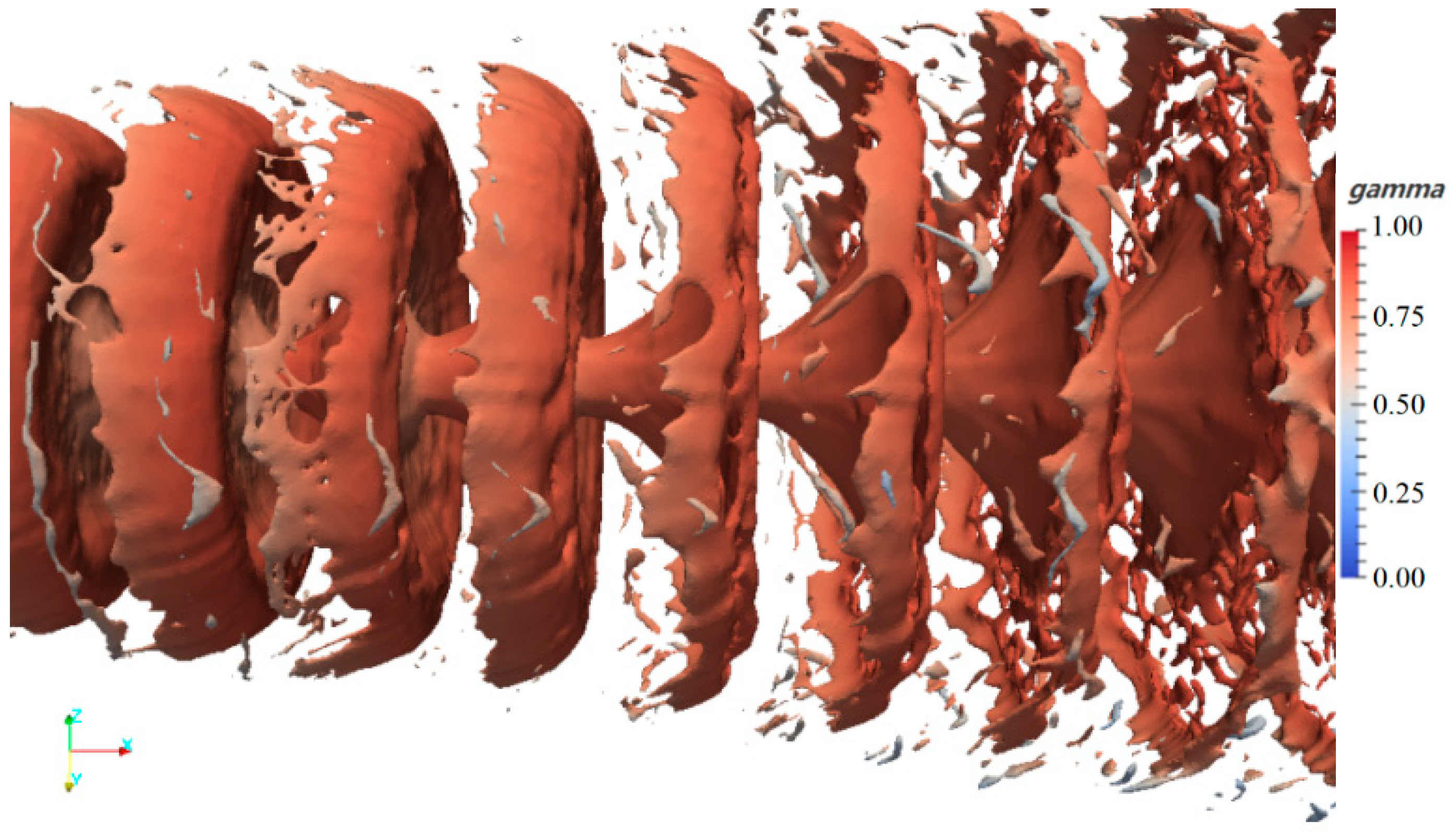
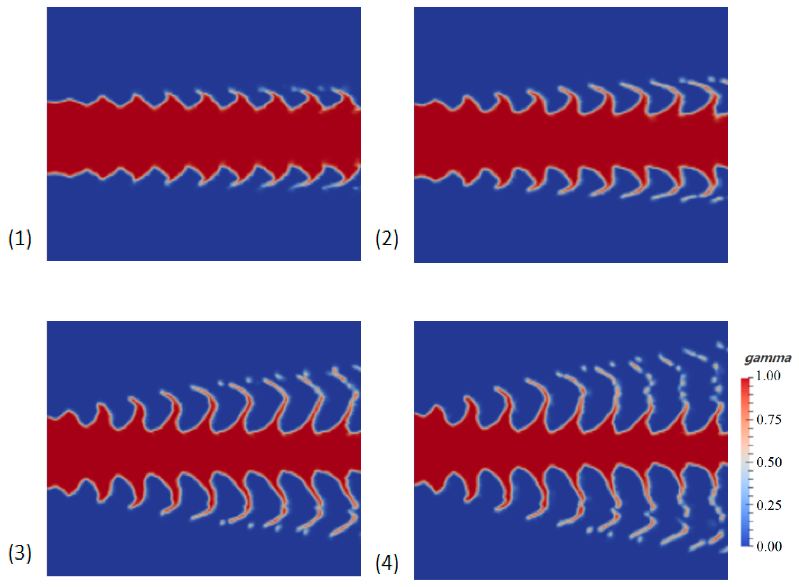
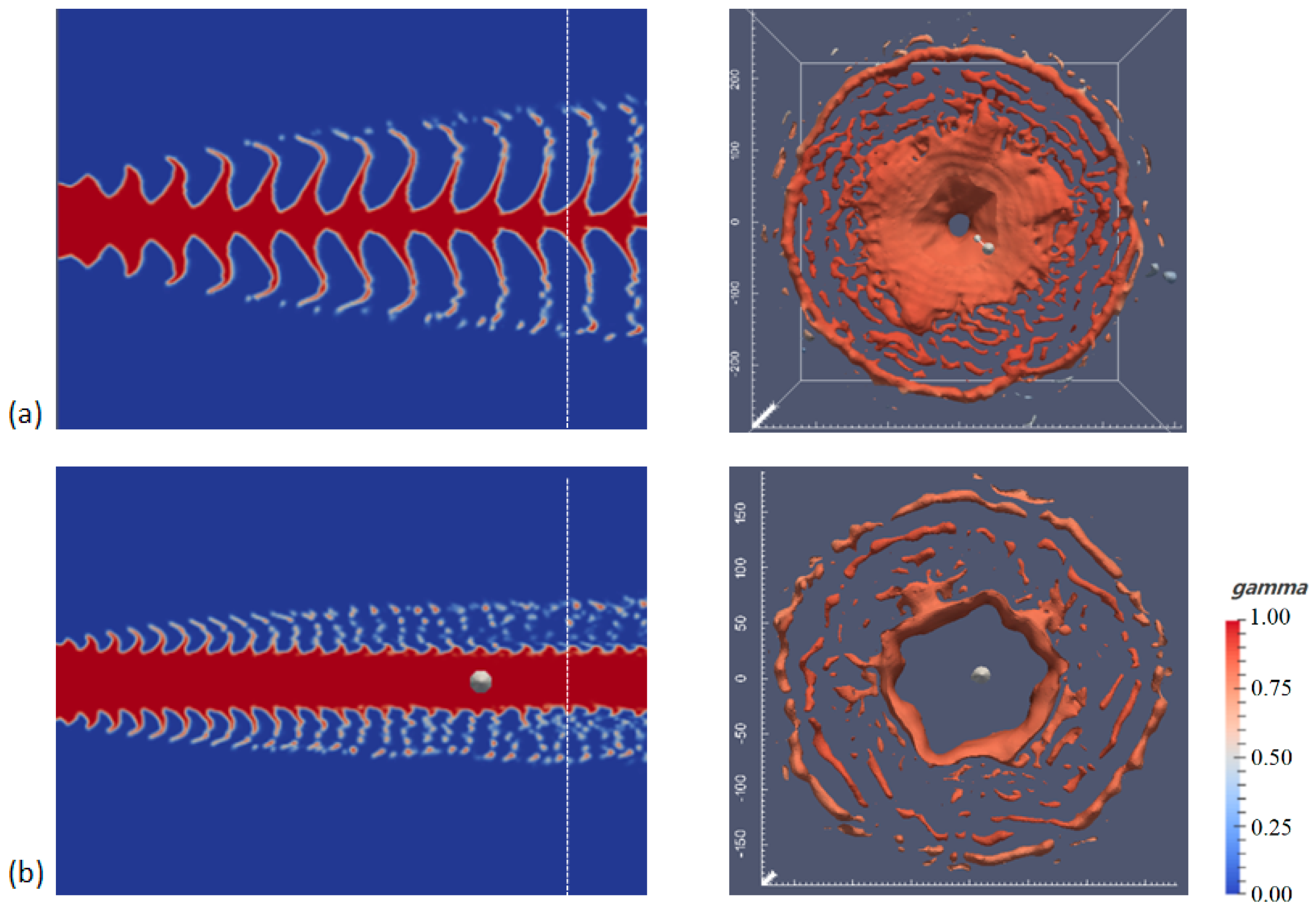
4.1. Structure of Disturbed Liquid Jet Sprays
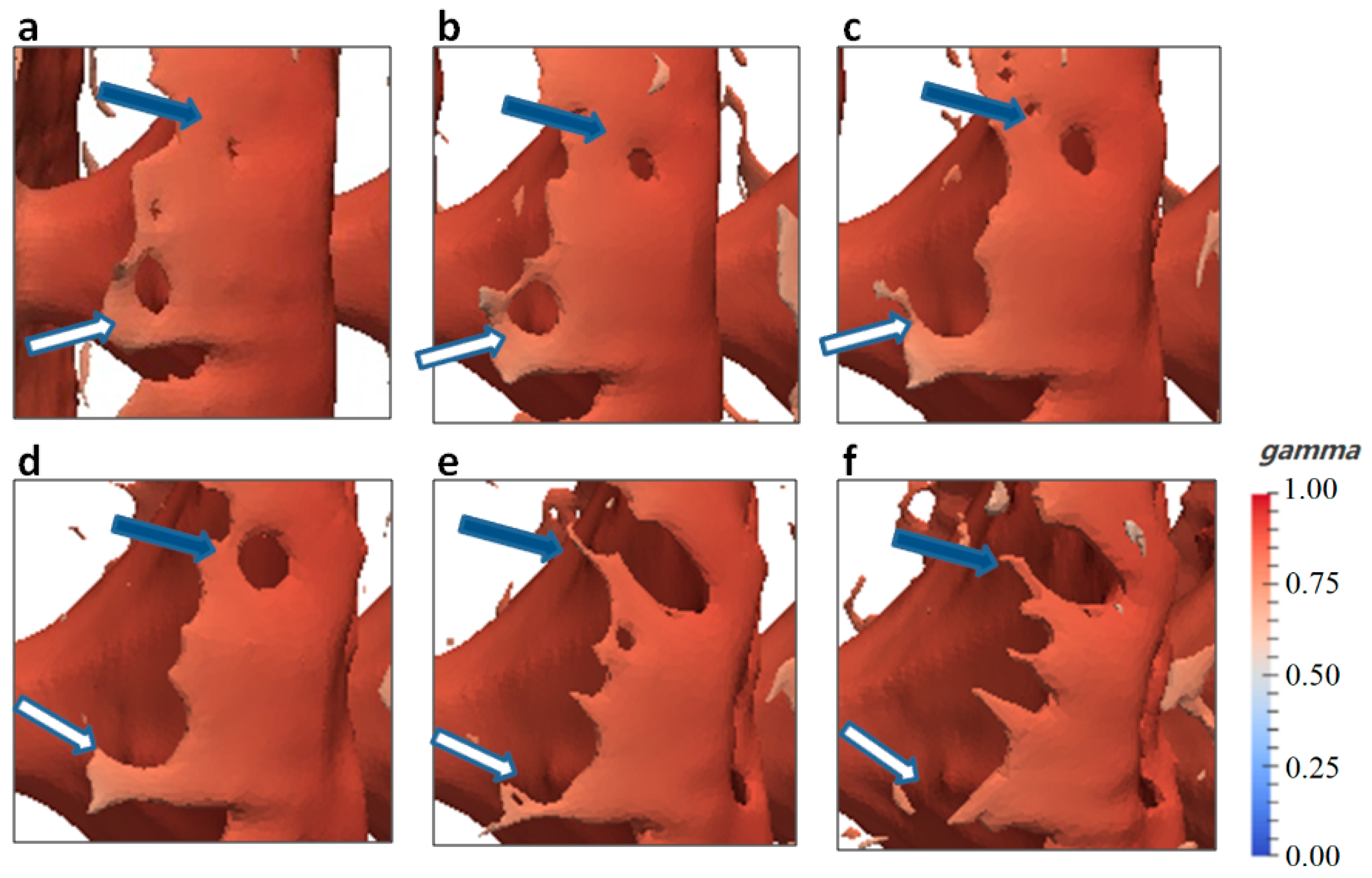
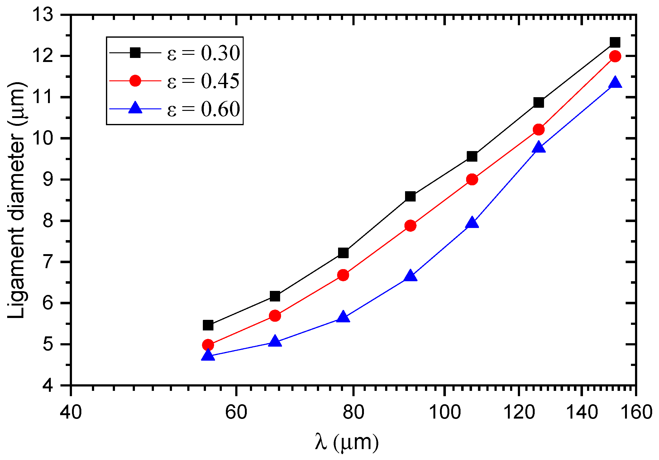
4.2. Ligament Formation from the Surface Wave
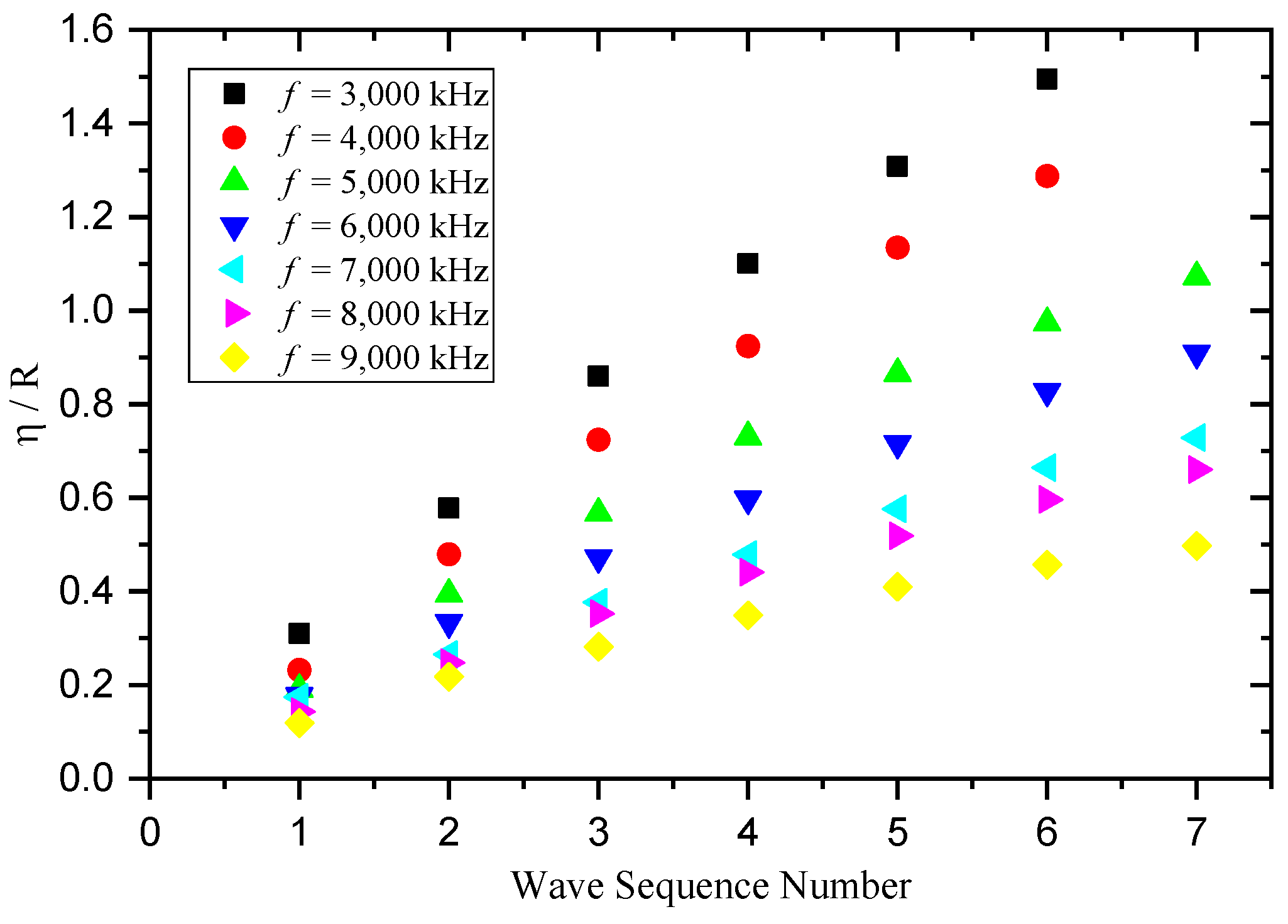
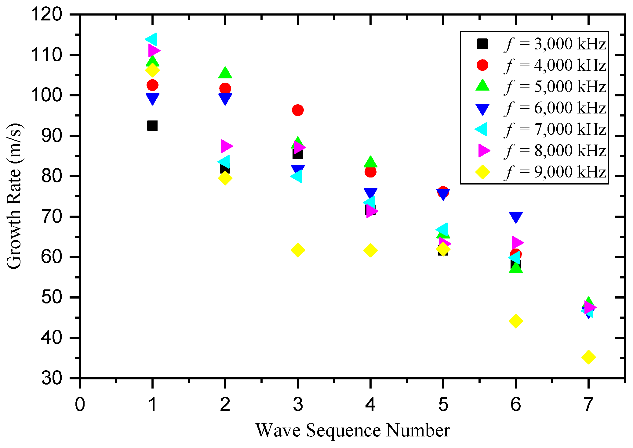
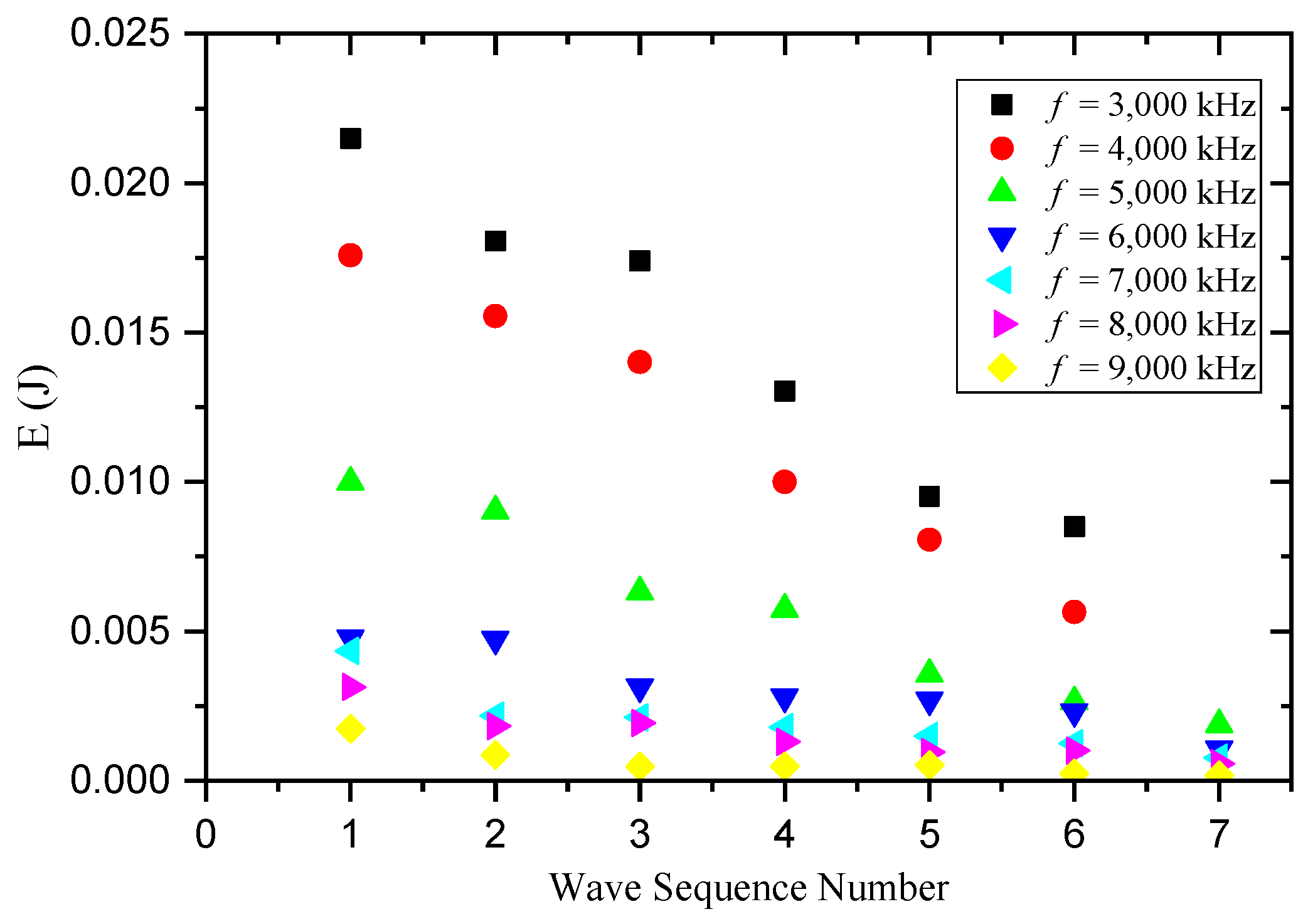
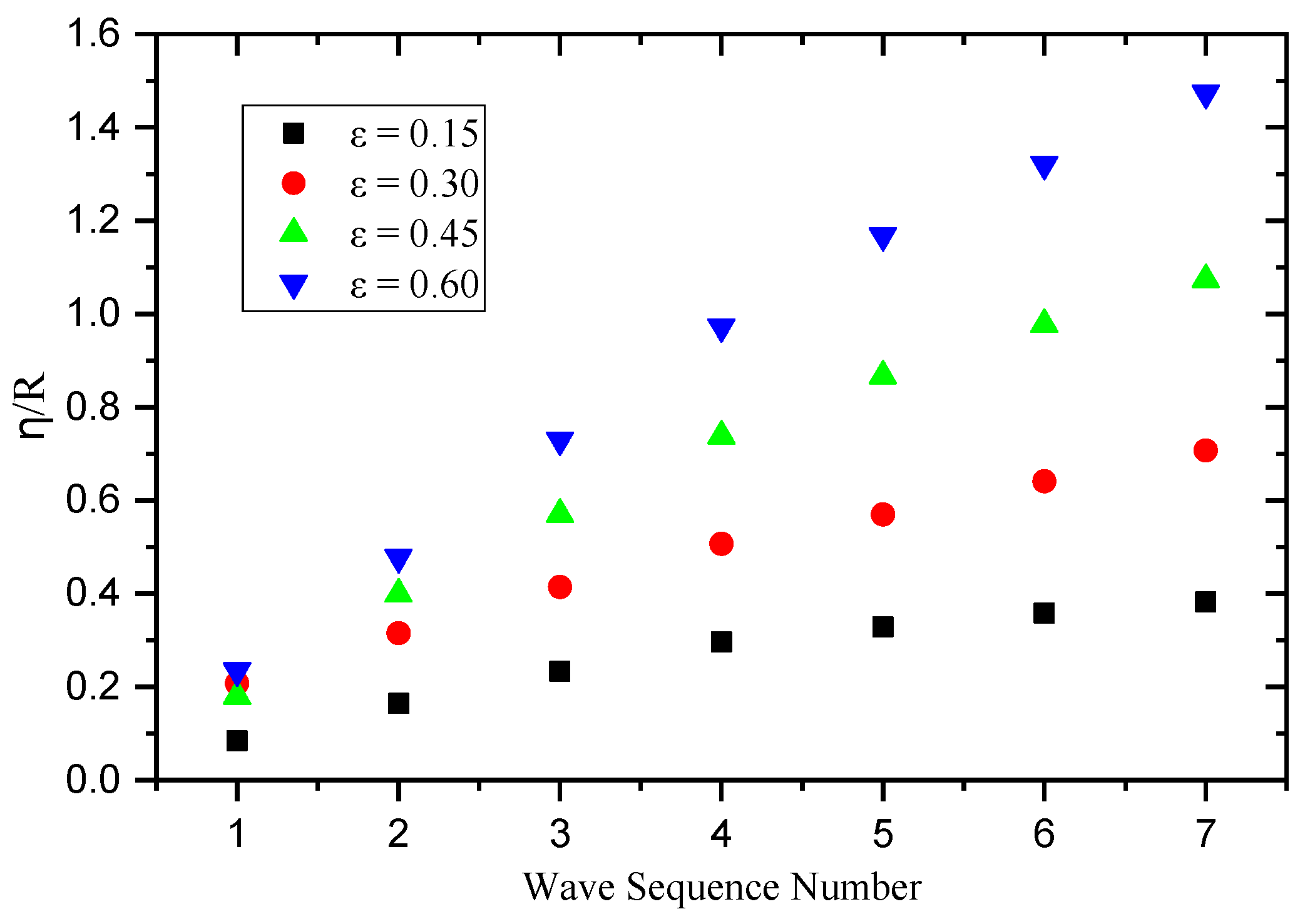
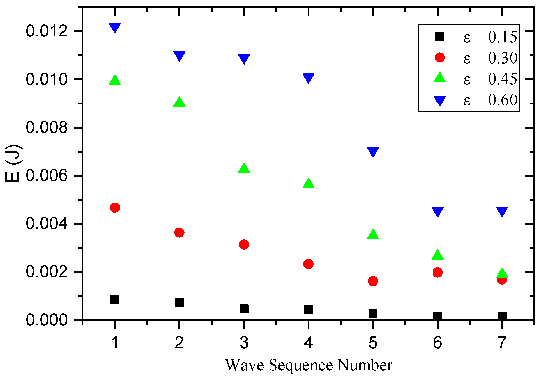
4.3. Characteristics of the Surface Wave
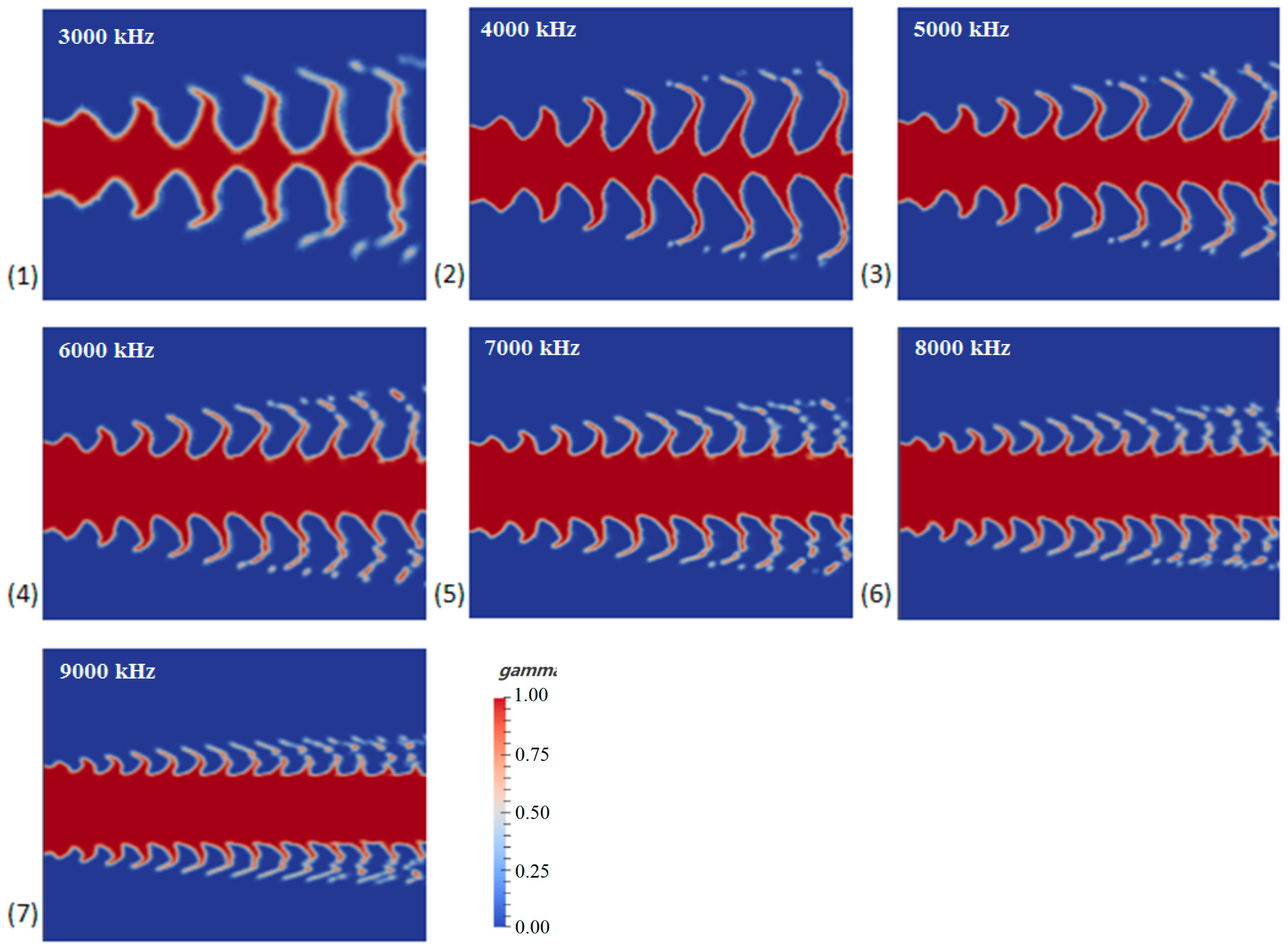
4.3.1. Analysis of Surface Wave Characteristics for Different Disturbance Frequencies
4.3.2. Analysis of the Surface Wave Characteristics for Different Disturbance Amplitudes
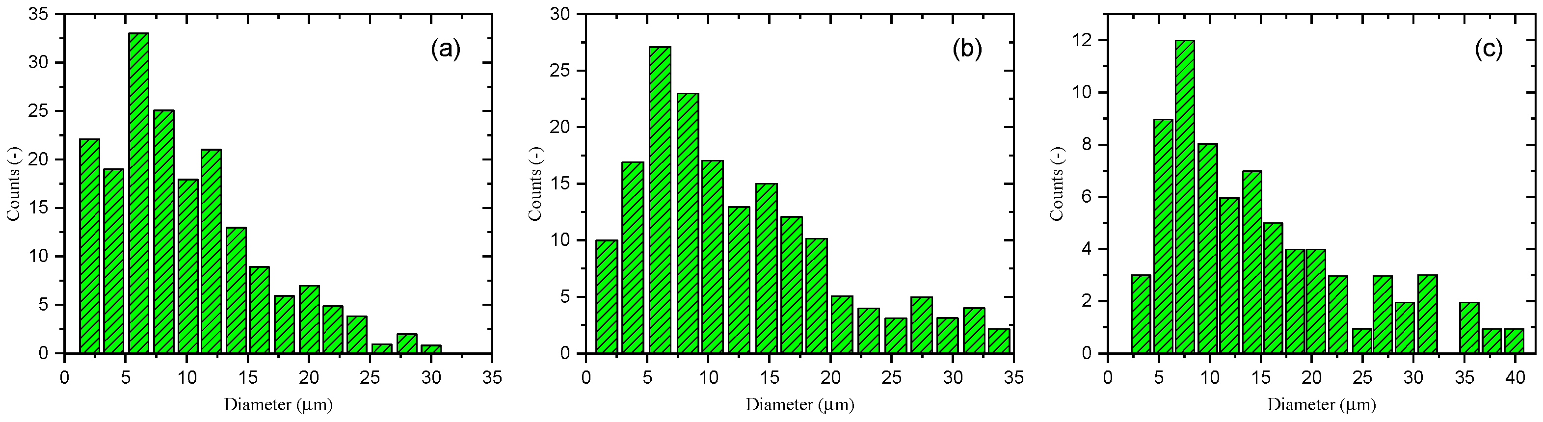
4.4. Length and Time Scales of Liquid Jet Primary Breakup
5. Conclusions
Author Contributions
Funding
Institutional Review Board Statement
Informed Consent Statement
Data Availability Statement
Conflicts of Interest
Nomenclature
| b | Characteristic length (m) |
| Liquid ligament diameter (m) | |
| Nozzle diameter (m) | |
| Kinetic energy (J) | |
| Disturbance frequency (1/s) | |
| Surface tension force (N) | |
| Mean thickness of the surface wave sheet (m) | |
| Turbulent kinetic energy (m2/s2) | |
| Normal vector | |
| Pressure (Pa) | |
| Primary breakup time (s) | |
| Time (s) | |
| T | Temperature (K) |
| Velocity (m/s) | |
| Axial velocity of liquid jet (m/s) | |
| Coordinate (m) | |
| Density (kg/m3) | |
| Dynamic viscosity (Pa·s) | |
| Subgrid scale (SGS) stress (m2/s2) | |
| SGS viscosity (N/m2) | |
| Mean strain rate tensor (s−1) | |
| Volume fraction | |
| Surface tension of the liquid (N/m) | |
| Curvature (1/m) | |
| Amplitude (m) | |
| Disturbance amplitude ratio | |
| Strouhal number | |
| Reynolds number | |
| Liquid–gas density ratio | |
| Weber number | |
| Subscripts | |
| Axial | Axial direction |
| cav | Cavitation |
| g | Gas |
| inj | Injection |
| i, j, k | Unit vectors in the x-, y-, and z-directions |
| l | Liquid |
| local | Local |
| max | Maximum |
| rad | Radial direction |
References
- Lin, S.P. Breakup of Liquid Sheets and Jets; Cambridge University Press: New York, NY, USA, 2003. [Google Scholar]
- Shinjo, J. Recent advances in computational modeling of primary atomization of liquid fuel sprays. Energies 2018, 11, 2971. [Google Scholar] [CrossRef] [Green Version]
- Chen, Y.; Chen, S.; Chen, W.; Hu, J.; Jiang, J. An Atomization Model of Air Spraying Using the Volume-of-Fluid Method and Large Eddy Simulation. Coatings 2021, 11, 1400. [Google Scholar] [CrossRef]
- Stahl, M.; Damaschke, N.; Tropea, C. Experimental investigation of turbulence and cavitation inside a pressure atomizer and optical characterization of the generated spray. In Proceedings of the 10th ICLASS Conference, Kyoto, Japan, 27 August–1 September 2006. [Google Scholar]
- Bagué, A.; Fuster, D.; Popinet, S. Instability growth rate of two-phase mixing layers from a linear eigenvalue problem and an initial-value problem. Phys. Fluids 2010, 22, 092104. [Google Scholar] [CrossRef] [Green Version]
- He, Z.; Guo, G.; Tao, X.; Zhong, W.; Leng, X.; Wang, Q. Study of the effect of nozzle hole shape on internal flow and spray characteristics. Int. Commun. Heat Mass 2016, 71, 1–8. [Google Scholar] [CrossRef]
- Suh, H.K.; Lee, C.S. Effect of cavitation in nozzle orifice on the diesel fuel atomization characteristics. Int. J. Heat Fluid Flow 2008, 29, 1001–1009. [Google Scholar] [CrossRef]
- Badock, C.; Wirth, R.; Fath, A. Investigation of cavitation in real size diesel injection nozzles. Int. J. Heat Fluid Flow 1999, 20, 538–544. [Google Scholar] [CrossRef]
- Shinjo, J.; Umemura, A. Simulation of liquid jet primary breakup: Dynamics of ligament and droplet formation. Int. J. Multiph. Flow 2010, 36, 513–532. [Google Scholar] [CrossRef]
- Shinjo, J.; Umemura, A. Surface instability and primary atomization characteristics of straight liquid jet sprays. Int. J. Multiph. Flow 2011, 37, 1294–1304. [Google Scholar] [CrossRef]
- He, Z.; Zhou, H.; Duan, L.; Xu, M.; Chen, Z.; Cao, T. Effects of nozzle geometries and needle lift on steadier string cavitation and larger spray angle in common rail diesel injector. Int. J. Engine Res. 2021, 22, 2673–2688. [Google Scholar] [CrossRef]
- Reitz, R.D.; Bracco, F.V. Mechanism of atomization of a liquid jet. Phys. Fluids 1982, 25, 1730. [Google Scholar] [CrossRef]
- Lin, S.P.; Reitz, R.D. Drop and spray formation from a liquid jet. Annu. Rev. Fluid Mech. 1998, 30, 85–105. [Google Scholar] [CrossRef]
- Zhao, W.; Yan, J.; Gao, S.; Lee, T.H.; Li, X. Effects of fuel properties and aerodynamic breakup on spray under flash boiling conditions. Appl. Therm. Eng. 2022, 200, 117646. [Google Scholar] [CrossRef]
- Schweitzer, P.H. Mechanism of disintegration of liquid jets. J. Appl. Phys. 1937, 8, 513–521. [Google Scholar] [CrossRef]
- Bergwerk, W. Flow pattern in diesel nozzle spray holes. Proc. Inst. Mech. Eng. 1959, 173, 655–660. [Google Scholar] [CrossRef]
- Chaves, H.; Knapp, M.; Kubitzek, A. Experimental study of cavitation in the nozzle hole of diesel injectors using transparent nozzles. SAE Trans. 1995, 104, 645–657. [Google Scholar]
- Soteriou, C. Direct Injection Diesel Spray and the Effect of Cavitation and Hydraulic Flip or Atomization. SAE Trans. 1995, 104, 128–153. [Google Scholar]
- Wei, Y.; Fan, L.; Zhang, H.; Gu, Y.; Deng, Y.; Leng, X.; Fei, H.; He, Z. Experimental investigations into the effects of string cavitation on diesel nozzle internal flow and near field spray dynamics under different injection control strategies. Fuel 2022, 309, 122021. [Google Scholar] [CrossRef]
- McCormack, P.D.; Crane, L.; Birch, S. An experimental and theoretical analysis of cylindrical liquid jets subjected to vibration. Br. J. Appl. Phys. 1965, 16, 395. [Google Scholar] [CrossRef]
- Chaves, H.; Obermeier, F.; Seidel, T. Fundamental investigation of the disintegration of a sinusoidally forced liquid jet. In Proceedings of the ICLASS-2000, Tsukuba, Japan, 13–15 December 2000; pp. 1018–1025. [Google Scholar]
- Geschner, F.; Obermier, G.; Chaves, H. Investigation of different phenomena of the disintegration of a sinusoidally forced liquid jet. In Proceedings of the Seventeenth Annual Conference on Liquid Atomization and Spray Systems, Zurich, Switzerland, 2–6 September 2001. [Google Scholar]
- Srinivasan, V.; Salazar, A.J.; Saito, K. Modeling the disintegration of modulated liquid jets using volume-of-fluid (VOF) methodology. Appl. Math. Model. 2011, 35, 3710–3730. [Google Scholar] [CrossRef]
- Srinivasan, V.; Salazar, A.J.; Saito, K. Numerical simulation of the disintegration of forced liquid jets using volume-of-fluid method. Int. J. Comput. Fluid Dyn. 2010, 24, 317–333. [Google Scholar] [CrossRef]
- Hwang, H.; Kim, D.; Moin, P. Atomization of the optimally disturbed liquid jet. Bull. Am. Phys. Soc. 2021, 66, 17. [Google Scholar]
- Zhou, C.; Zou, J.; Zhang, Y. Effect of Streamwise Perturbation Frequency on Formation Mechanism of Ligament and Droplet in Liquid Circular Jet. Aerospace 2022, 9, 191. [Google Scholar] [CrossRef]
- Linne, M.; Paciaroni, M.; Hall, T. Ballistic imaging of the near field in a diesel spray. Exp. Fluids 2006, 40, 836–846. [Google Scholar] [CrossRef]
- Blaisot, J.B.; Yon, J. Droplet size and morphology characterization for dense sprays by image processing: Application to the Diesel spray. Exp. Fluids 2005, 39, 977–994. [Google Scholar] [CrossRef]
- Wang, Y.; Liu, X.; Im, K.S. Ultrafast X-ray study of dense-liquid-jet flow dynamics using structure-tracking velocimetry. Nat. Phys. 2008, 4, 305–309. [Google Scholar] [CrossRef] [Green Version]
- Salvador, F.J.; Gimeno, J.; De La Morena, J.; González-Montero, L.A. Experimental analysis of the injection pressure effect on the near-field structure of liquid fuel sprays. Fuel 2021, 292, 120296. [Google Scholar] [CrossRef]
- Payri, R.; Gimeno, J.; Martí-Aldaraví, P.; Martínez, M. Transient nozzle flow analysis and near field characterization of gasoline direct fuel injector using Large Eddy Simulation. Int. J. Multiph. Flow 2022, 148, 103920. [Google Scholar] [CrossRef]
- Mukundan, A.A.; Ménard, T.; De Motta, J.C.B.; Berlemont, A. Detailed numerical simulations of primary atomization of airblasted liquid sheet. Int. J. Multiph. Flow 2022, 147, 103848. [Google Scholar] [CrossRef]
- Ménard, T.; Tanguy, S.; Berlemont, A. Coupling level set/VOF/ghost fluid methods: Validation and application to 3D simulation of the primary break-up of a liquid jet. Int. J. Multiph. Flow 2007, 33, 510–524. [Google Scholar] [CrossRef]
- Desjardins, O.; Moureau, V.; Pitsch, H. An accurate conservative level set/ghost fluid method for simulating turbulent atomization. J. Comput. Phys. 2008, 227, 8395–8416. [Google Scholar] [CrossRef]
- De Villiers, E.; Gosman, A.D.; Weller, H.G. Large eddy simulation of primary diesel spray atomization. SAE Trans. 2004, 113, 193–206. [Google Scholar]
- Pai, M.G.; Desjardins, O.; Pitsch, H. Detailed simulations of primary breakup of turbulent liquid jets in crossflow. Cent. Turbul. Res. Annu. Res. Briefs 2008, 34, 451–466. [Google Scholar]
- Herrmann, M. A balanced force refined level set grid method for two-phase flows on unstructured flow solver grids. J. Comput. Phys. 2008, 227, 2674–2706. [Google Scholar] [CrossRef]
- Herrmann, M. Detailed numerical simulations of the primary breakup of turbulent liquid jets. In Proceedings of the 21st Annual Conference of ILASS Americas, Orlando, FL, USA, 18–21 May 2008; pp. 1–17. [Google Scholar]
- Herrmann, M. The impact of density ratio on the primary atomization of a turbulent liquid jet in crossflow. Bull. Am. Phys. Soc. 2009, 54, 191–205. [Google Scholar]
- Liu, K.; Huck, P.D.; Aliseda, A.; Balachandar, S. Investigation of turbulent inflow specification in Euler–Lagrange simulations of mid-field spray. Phys. Fluids 2021, 33, 033313. [Google Scholar] [CrossRef]
- Daskiran, C.; Xue, X.; Cui, F.; Katz, J.; Boufadel, M.C. Impact of a jet orifice on the hydrodynamics and the oil droplet size distribution. Int. J. Multiph. Flow 2022, 147, 103921. [Google Scholar] [CrossRef]
- Apte, S.V.; Gorokhovski, M.; Moin, P. LES of atomizing spray with stochastic modeling of secondary breakup. Int. J. Multiph. Flow 2003, 29, 1503–1522. [Google Scholar] [CrossRef]
- Ubbink, O. Numerical Prediction of Two Fluid Systems with Sharp Interfaces. Ph.D. Thesis, University of London, London, UK, 1997. [Google Scholar]
- Brackbill, J.U.; Kothe, D.B.; Zemach, C. A continuum method for modeling surface tension. J. Comput. Phys. 1992, 100, 335–354. [Google Scholar] [CrossRef]
- Martínez, J.; Piscaglia, F.; Montorfano, A.; Onorati, A.; Aithal, S.M. Influence of momentum interpolation methods on the accuracy and convergence of pressure–velocity coupling algorithms in OpenFOAM®. J. Comput. Appl. Math. 2017, 309, 654–673. [Google Scholar] [CrossRef]
- Blessing, M.; König, G.; Krüger, C. Analysis of flow and cavitation phenomena in Diesel injection nozzles and its effects on spray and mixture formation. SAE Trans. 2003, 112, 1694–1706. [Google Scholar]
- Ghiji, M.; Goldsworthy, L.; Brandner, P.A.; Garaniya, V.; Hield, P. Analysis of diesel spray dynamics using a compressible Eulerian/VOF/LES model and microscopic shadowgraphy. Fuel 2017, 188, 352–366. [Google Scholar] [CrossRef] [Green Version]
- Martinez, L.; Benkenida, A.; Cuenot, B. A model for the injection boundary conditions in the context of 3D simulation of diesel spray: Methodology and validation. Fuel 2010, 89, 219–228. [Google Scholar] [CrossRef]
- Huh, K.Y.; Lee, E.; Koo, J. Diesel Spray Atomization Model Considering Nozzle Exit Turbulence Conditions. At. Sprays 1998, 8, 453–469. [Google Scholar] [CrossRef]
- Baumgarten, C.; Stegemann, J.; Merker, G.P. A New Model for Cavitation Induced Primary Break-up of Diesel Sprays. In Proceedings of the ILASS-Europe 2002, Zaragoza, Spain, 9 September–9 November 2002. [Google Scholar]
- Sarre, C.; Kong, S.C.; Reitz, R.D. Modeling the effects of injector nozzle geometry on diesel sprays. SAE Pap. 1999, 108, 1375–1388. [Google Scholar]
- Gao, J.; Park, S.W.; Wang, Y.; Reitz, R.D.; Moon, S.; Nishida, K. Simulation and analysis of group-hole nozzle sprays using a gas jet superposition model. Fuel 2010, 89, 3758–3772. [Google Scholar] [CrossRef]
- Lin, S.P.; Kang, D.J. Atomization of a liquid jet. Phys. Fluids 1987, 30, 2000. [Google Scholar] [CrossRef]
- Lin, S.P.; Lian, Z.W. Mechanisms of the breakup of liquid jets. AIAA J. 1990, 28, 120–126. [Google Scholar] [CrossRef]
- Ranz, W.E. On Sprays and Spraying; College of Engineering and Architecture: Washindgton, DC, USA, 1959. [Google Scholar]


| Parameters | Value |
|---|---|
| Nozzle diameter (mm) | 0.2 |
| Ambient pressure (MPa) Ambient temperature (K) | 0.1 298.15 |
| Gas density (kg/m3) | 1.29 |
| Liquid density (kg/m3) | 840 |
| Gas dynamic viscosity (Pa·s) | 1.79 × 10⁻⁵ |
| Liquid kinematic viscosity (m2/s) | 2.87 × 10⁻⁶ |
| Surface tension coefficient (N/m) | 0.026 |
| Injection pressure (MPa) Injecting velocity of liquid jet (m/s) | 80 336 |
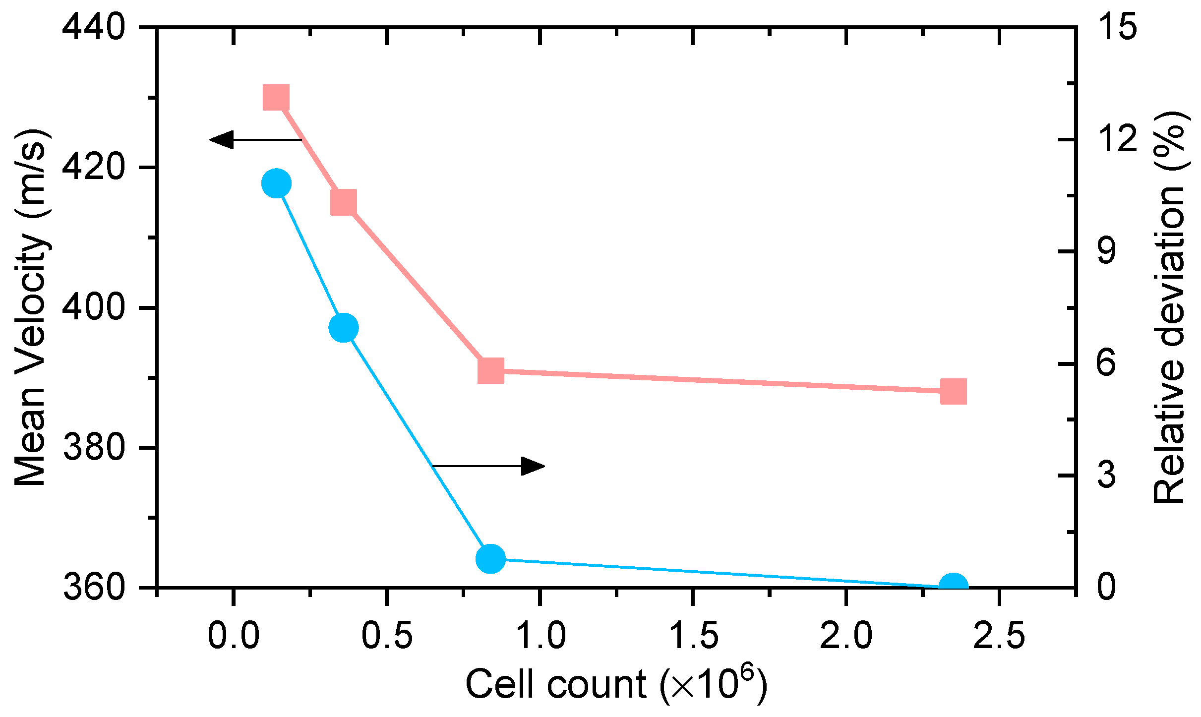
| Case | Initial Average Grid Size, μm | Cell Count | Time Step, ns | CPU (Core Count) | Wall Clock Time, h | Final Average Grid Size, μm |
|---|---|---|---|---|---|---|
| Very coarse | 40 | 0.14 × 10⁶ | 0.5 ≤ Δt ≤ 2 | 72 | 35 | 18.9 |
| Coarse | 20 | 0.36 × 10⁶ | 0.5 ≤ Δt ≤ 2 | 72 | 64 | 9.7 |
| Medium | 12 | 0.84 × 10⁶ | 0.5 ≤ Δt ≤ 2 | 72 | 120 | 5.6 |
| Fine | 6 | 2.35 × 10⁶ | 0.5 ≤ Δt ≤ 2 | 72 | 282 | 2.8 |
Publisher’s Note: MDPI stays neutral with regard to jurisdictional claims in published maps and institutional affiliations. |
© 2022 by the authors. Licensee MDPI, Basel, Switzerland. This article is an open access article distributed under the terms and conditions of the Creative Commons Attribution (CC BY) license (https://creativecommons.org/licenses/by/4.0/).
Share and Cite
Liu, Z.; Li, Z.; Liu, J.; Wu, J.; Yu, Y.; Ding, J. Numerical Study on Primary Breakup of Disturbed Liquid Jet Sprays Using a VOF Model and LES Method. Processes 2022, 10, 1148. https://doi.org/10.3390/pr10061148
Liu Z, Li Z, Liu J, Wu J, Yu Y, Ding J. Numerical Study on Primary Breakup of Disturbed Liquid Jet Sprays Using a VOF Model and LES Method. Processes. 2022; 10(6):1148. https://doi.org/10.3390/pr10061148
Chicago/Turabian StyleLiu, Zhenming, Ziming Li, Jingbin Liu, Jiechang Wu, Yusong Yu, and Jiawei Ding. 2022. "Numerical Study on Primary Breakup of Disturbed Liquid Jet Sprays Using a VOF Model and LES Method" Processes 10, no. 6: 1148. https://doi.org/10.3390/pr10061148