Article

Multi-Objective Optimization of a Crude Oil Hydrotreating Process with a Crude Distillation Unit Based on Bootstrap Aggregated Neural Network Models

School of Engineering, Merz Court, Newcastle University, Newcastle upon Tyne NE1 7RU, UK
*
Author to whom correspondence should be addressed.
Processes 2022, 10(8), 1438; https://doi.org/10.3390/pr10081438
Submission received: 21 June 2022 / Revised: 18 July 2022 / Accepted: 20 July 2022 / Published: 22 July 2022

Abstract

:
This paper presents the multi-objective optimization of a crude oil hydrotreating (HDT) process with a crude atmospheric distillation unit using data-driven models based on bootstrap aggregated neural networks. Hydrotreating of the whole crude oil has economic benefit compared to the conventional hydrotreating of individual oil products. In order to overcome the difficulty in developing accurate mechanistic models and the computational burden of utilizing such models in optimization, bootstrap aggregated neural networks are utilized to develop reliable data-driven models for this process. Reliable optimal process operating conditions are derived by solving a multi-objective optimization problem incorporating minimization of the widths of model prediction confidence bounds as additional objectives. The multi-objective optimization problem is solved using the goal-attainment method. The proposed method is demonstrated on the HDT of crude oil with crude distillation unit simulated using Aspen HYSYS. Validation of the optimization results using Aspen HYSYS simulation demonstrates that the proposed technique is effective.

1. Introduction

Oil and gas are among the most widely utilized natural resources in modern society. Crude oil is a mixture of different hydrocarbons and small quantities of sulphur, nitrogen, and some metal elements [1]. Refined oil products provide fuels for modern transportation, such as automobiles, airplanes, and ships. In addition to being used as fuels, oil products also provide raw materials for the chemical industry in the production of a wide range of products with the most well known as various types of plastics. Crude oil needs to be split into more valuable products by distillation processes in the oil refinery. The purpose of the oil-refining process is to separate crude oil (raw material) into different types of oil products, such as light gas oil, jet fuels, light naphtha, kerosene, etc. Figure 1 shows a flowsheet of a typical crude oil refinery [2,3], which is a complex process containing many processing units, such as crude distillation units (CDU), reformer units, hydrotreating units (HDT), fluid catalytic cracking (FCC), vacuum distillation units (VDU), hydrocracking units (HCU), and others. In addition, there are some offsite facilities, such as tank farms, pipe systems, traps and depots. Refineries are large and complex processes and consume large amounts of energy and water.
Crude oil from different oil fields around the world varies in composition as well as containing undesirable impurities, such as sulphur and nitrogen. The undesirable impurities in oil products need to be removed or reduced due to strict environmental regulations for limiting sulphur and nitrogen contents in oil products. As a matter of fact, oil products with high sulphur content can lead to corrosion, pollution, and poisoning to catalyst. Thus, it is important to reduce the sulphur content in oil products. In crude oil refineries, the process for reducing sulphur compounds is known as hydrodesulphurization (HDS) while that for reducing nitrogen compounds is known as hydrodenitrogenation (HDN) [4]. The hydrodemetallization (HDM) process is responsible for removing nickel and vanadium contaminants from the heavy feed. The hydrotreating (HDT) process is employed to remove sulphur, nitrogen, and aromatic saturation compounds [5].
The conventional approach is to apply HDT on some individual oil products. In order to improve refinery efficiency, a few researchers have investigated applying HDT to the crude oil instead of individual oil products recently [6,7]. HDT of crude oil is a new hydrotreating process that has not been extensively reported and it has economic benefit compared to the conventional HDT process [8]. Jarullah et al. [6] shows that this new hydrotreating process can significantly improve middle distillate yields. Moreover, the desulphurization of whole crude oil has the potential to more effectively meet the need of environmental legislation for decreasing sulphur content and producing clean fuels in the refining processes and is expected to become more common in the future [7].
Optimal operating conditions for crude oil HDT process need to be determined in order to obtain the best process operation performance. A number of process variables can be considered as the decision variables in the optimization of crude oil HDT process. Table 1 shows the operating conditions of different HDT technologies applied to different oil products [9]. The process variables shown in Table 1, pressure (P), temperature (T), liquid hourly space velocity (LHSV), and hydrogen-to-hydrocarbon (H2/HC) ratio can be considered as the decision variables in optimizing crude oil HDT process.
Optimizing crude oil HDT processes will require an accurate process model. It is generally very difficult to obtain accurate mechanistic models for crude oil HDT processes due to the complexity of the material and process involved. To overcome this difficulty, data-driven models obtained from process operation data should be utilized. In recent years, there has been an increasing interest in computational intelligence, particularly in the area of machine learning, which has contributed significantly to data-driven modelling. Among the machine-learning tools, neural networks are a very powerful tool for data-driven modelling. They attempt to mimic the way in which the human brain functions. A neural network consists of a number of information-processing units named neurons which are arranged into layers. Neurons in adjacent layers are connected through weighted connections. During neural network training, the neural network weights are adjusted so that the neural network can learn the relationship between the input and output data. Advanced versions of neural networks, such as stacked neural networks, extreme learning machines, and deep learning, have also been applied to nonlinear process modelling [10,11,12,13,14].
In this work, bootstrap aggregated neural networks are employed to model a crude oil HDT with the CDU process and then used to optimize the process operation. Simulated process operation data are obtained from Aspen HYSYS simulation and used for developing bootstrap aggregated neural network models. Note that simulated process operation data are used here to represent real plant operation data. When real plant operation data are available, they can be directly used to build neural network models. The developed bootstrap aggregated neural network models are then utilized in a multi-objective optimization framework. In order to enhance the reliability of optimization results, minimizing the widths of model prediction confidence bounds is considered as a further optimization objective. The multi-objective optimization problem is solved by using the goal-attainment method. In some cases, even the Aspen HYSYS models are available, and their neural network surrogate models are often used in the optimization due to the short computation time of neural network models. This type of surrogate modelling approach has been getting popular in recent years [15]. A recent study on reducing the computational burden of mechanistic models using analytical simplifications could enable real-time optimization with mechanistic models in some cases [16].
The novelty of this study lies in the following two areas. First, reliable data-driven models are developed from a limited amount of simulated process operation data through utilizing bootstrap aggregated neural networks. Secondly, a reliable multi-objective optimization framework for a crude oil HDT with the CDU process is developed through utilizing the model prediction confidence bounds.
This paper is structured as follows: Section 2 provides process description for the crude oil HDT process with CDU. Also, the crude oil feedstock and products specifications are given in this section. Modelling of a crude oil HDT with the CDU process using bootstrap aggregated neural networks is detailed in Section 3. Section 4 presents multi-objective optimization of the crude oil HDT with the CDU process using the goal-attainment method. The last section gives some concluding remarks.

2. A Crude Oil HDT Process with CDU

2.1. Process Description

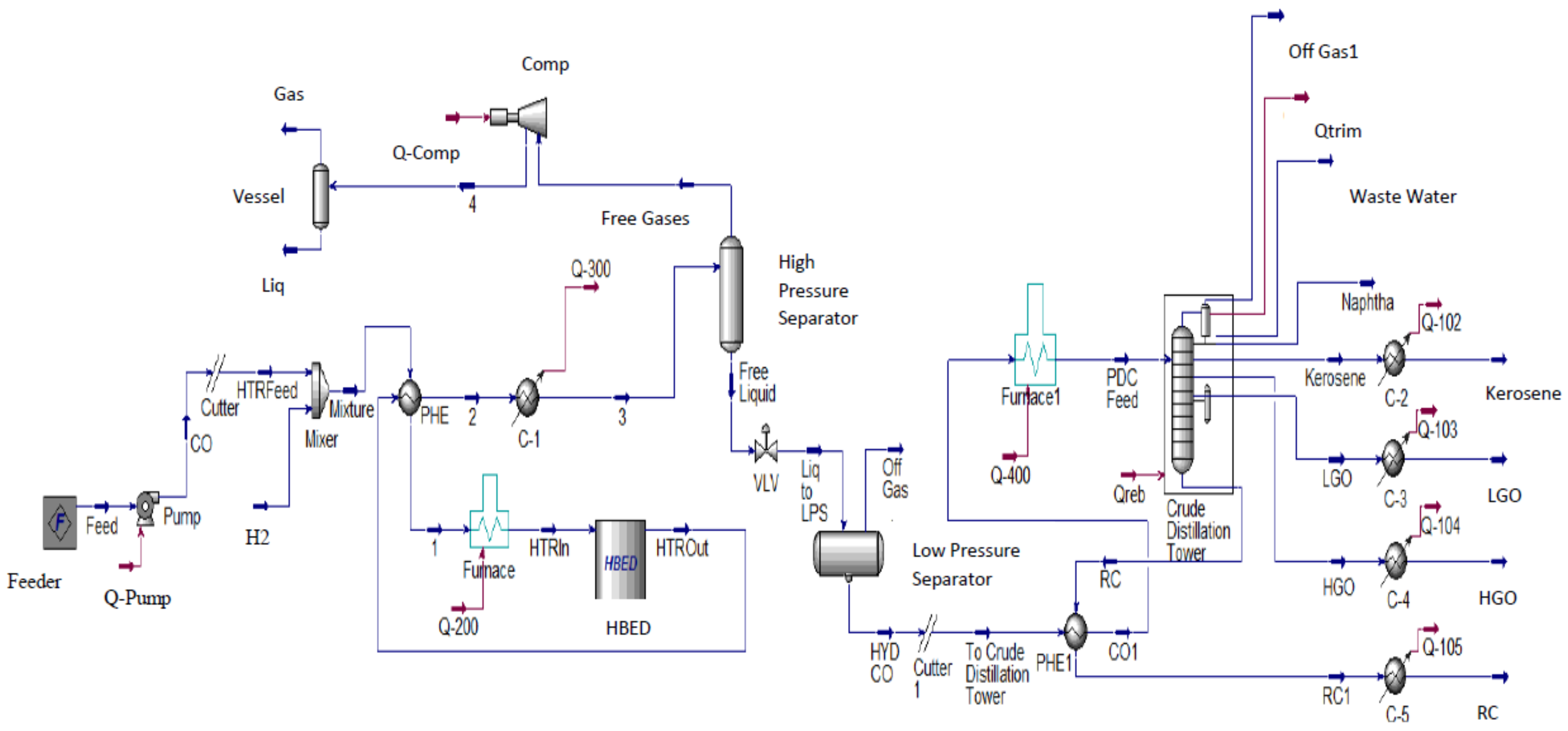
The process flow diagram of crude oil HDT process with CDU is illustrated in Figure 2. At the beginning, crude oil is taken from storage tanks and is joined by a stream of hydrogen gas. The mixture is fed to a train of heat-exchangers where they are pre-heated. After that, the mixture enters the convection and radiation sections of a furnace where they are heated to the required reaction temperature and then are fed to a reactor containing catalysts (HBED in Figure 2). The reactor effluent is employed to preheat the charge (crude oil) by the heat-exchanging system. Then the effluent is cooled in a cooler. Following that, the mixture of liquid and gases is fed into a high-pressure separator where gases, such as hydrogen sulphide and unreacted hydrogen, are removed from the liquid. The gases are then compressed and sent to a vessel whereas the liquid passes to a low-pressure separator to further remove gases not being removed in the high-pressure separator. After that, the hydrotreated crude oil is fed to a CDU process. Aspen HYSYS with the Peng–Robinson fluid package is employed to simulate the process. The CDU is designed to be able to cope with the maximum crude feed rate considered to prevent column flooding so that the optimization study will not be affected by the hydraulic limitation. The CDU considered here has 29 trays with 0.5 m tray spacing.
In general, the function of the crude distillation unit is to distil and split the feedstock into different types of oil products, such as off gas, naphtha (N), kerosene (K), light gas oil (LGO), heavy gas oil (HGO), and reduced crude (RC). The hydrotreated crude oil is preheated in the train of heat-exchangers and then fed to the furnace where it is finally heated to the required temperature and vaporized. The mixed liquid and vapor charge flows to the flash zone of the crude distillation tower. Liquid from the flash zone flows across many stripping trays in the bottom section of the tower. Additionally, stripping steam is injected to increase vaporization and reduce volatile content and in this way to remove lighter compounds. Vapors leaving the flash zone pass through the wash section of the tower and they are further condensed and fractionated on the trays of a fraction section with two pump-around sections to yield side-drawn products. The total naphtha leaves the column via the column top and accumulates in the overhead drum after condensation. From the overhead drum, part of the naphtha is recycled back to the tower top and the rest is pumped to the naphtha stabilizer as a product. The side products of the distillation tower (K, LGO, and HGO) flow to the stripper tower sections where they are individually steam-stripped to remove dissolved lighter components which are returned to the tower. Each side product (K, LGO, and HGO) is cooled and sent by pump to the storage tanks. Finally, RC from the tower bottom is used to preheat the hydrotreated crude oil (charge) and further cooled by the cooler and then sent to the storage tanks.

2.2. Feed and Products Specifications

Generally, there are specific chemical and physical properties for each type of crude oil. These characteristics include refinery-related specifications, such as PONA analysis, specific gravity, pour point, kinematic viscosity, and sulphur and nitrogen contents. The data involved in a petroleum assay includes yields produced from the physical distillate and residue properties [17]. The feed and product specifications are given in Table 2 [18] and Table 3, respectively. In this work, the products’ specifications were taken from the Midland Refineries Company (Daura Refinery). Crude oil products and the ranges of hydrocarbons in each fraction are illustrated in Table 4 [19].

3. Modelling of the Crude Oil HDT Process with CDU Using Bootstrap Aggregated Neural Networks

HDT process optimization should be carried out in order to enhance process efficiency. Accurate process models are essential for process optimization. Process models can be broadly divided into mechanistic models and data-driven models. The development of detailed mechanistic models is typically very time-consuming. Furthermore, optimization using mechanistic models in the form of differential and algebraic equations is also computationally demanding. In some cases, where even a mechanistic model is available, data-driven surrogate models are used in process optimization [15,20]. In building such data-driven surrogate models, detailed mechanistic models are used to simulate process operation under various operating conditions and the simulated process operation data are used in the development of data-driven surrogate models which are computationally efficient in solving process optimization problems.
The goal of HDT of crude oil with the CDU scheme is to minimize undesirable impurities, for instance, sulphur and some other compounds in the treated kerosene produced from the main atmospheric column. To overcome the difficulties in developing detailed mechanistic models, as well as using them in process optimization, neural network models are developed from process operation data. An Aspen HYSYS-based process simulator was used to produce various process operation data under different operating conditions of the HDT of crude oil with the CDU process. When sufficient plant operation data are available, then data reconciliation can be applied so that the Aspen HYSYS can match with real plant operation data [21]. Then, the data were utilized to construct neural network models. It should be noted that when real plant operation data are available, then they can be directly used in building neural network models.
As the main purpose of the developed neural network models is for process optimization, the neural network inputs and outputs should be selected so that they can be used in process optimization, i.e., they should be related to the optimization objective function and decision variables. In this work, the neural network inputs are selected as the flow rates of crude oil and hydrogen, and the pressure and temperature of the reactor. These are important process operation variables and can be measured and adjusted during process operation. The neural network outputs are selected as the contents of sulphur and nitrogen in the kerosene produced from the CDU, which will be minimized in the optimization problem. In this work, two neural network models are developed and they are represented by the following equations:
S = f1(x1, x2, x3, x4)
N = f2(x1, x2, x3, x4)
where S and N are the contents of sulphur and nitrogen, respectively, in the kerosene produced from the CDU, and x1 to x4 are, respectively, flow rates of crude oil and hydrogen, reactor pressure, and temperature.
The development of neural network models for predicting sulphur and nitrogen contents in the treated kerosene comprise four essential steps. The first step is the collection of data for model building. The second step is data normalization and data partition into training data, testing data, and unseen validation data. The third step is to select the structure of neural networks, such as the number of hidden neurons, layers, and the type of transfer functions. The fourth step is the training and validation of the neural networks.
In this study, 197 data samples are generated from the Aspen HYSYS simulation of a crude oil HDT process with CDU to develop neural network models. The data samples are generated by varying the crude oil flow rate, hydrogen flow rate, and reactor pressure and temperature within their constraints and they cover the range of inputs over which the optimization is carried out. The lower and upper bounds of these variables are given in Table 5. To represent the practical situations where process operation data are limited, a relatively small amount of simulated plant operation data are produced through simulation. To address the issue of different magnitudes in the model input and output variables, all input and output data are scaled to zero mean and unit variance before they are used in network training. In order to represent practical situations, simulated measurement noises are added to the simulated plant operation data. The simulated measurement noises follow normal distribution with zero means. In this study, the standard deviations for the measurement noises on feed flow rate, H2 molar flow rate, reactor pressure and temperature, and sulphur and nitrogen contents are, respectively, 0.3 m3/h, 1.5 kgmole/h, 0.5 bar, 0.3 °C, 0.003 Wt.%, and 1.5 ppmwt. Note that these measurement noises are only added to the outputs from the Aspen HYSYS simulation, not to any inputs to the Aspen HYSYS simulation. The data are split into three groups: training data (56%), testing data (23%), and unseen validation data (21%). The networks are trained on the training data. The testing data are utilized for the determination of network structure and early termination of the training process to avoid over-fitting. The final developed model is evaluated on the unseen validation data. As mentioned earlier, the simulated process operation data represent the practical situations where the available process operation data may not be abundant. Therefore, a relatively large portion of the data are used as training data. On the other hand, if the neural network models are used as surrogate models for the mechanistic model (Aspen HYSYS model), then plenty of data can be generated and a large portion of the data should be used as testing and validation data.

3.1. Single Neural Network Models

In this work, single neural network models are developed first for the purpose of comparison. The networks have a single hidden layer as a single hidden layer network can approximate any continuous nonlinear function [22]. The activation function in the hidden neurons is the sigmoid whereas that in the output layer is the linear activation function. The networks are trained using the Levenberg–Marquardt training algorithm with regularization and early stopping to avoid over-fitting. During the process of network training, network errors on the testing data are continuously monitored and training is terminated when testing errors stop decreasing. The initial network weights are taken as random values uniformly distributed in the range (−0.1, 0.1), and the regularization parameter is selected as 0.1. The number of hidden neurons is determined by trying a number of neural networks with a range of hidden neurons (from 2 to 30) and examining their sum of squared errors (SSE) on the testing data. The network with the least SSE on the testing data is considered as having the appropriate number of hidden neurons. Figure 3 depicts the neural network model performance on the training, testing, and unseen validation data for modelling the contents of sulphur and nitrogen in treated kerosene from the HDT of crude oil with CDU. It can be seen that there are a few noticeable errors on the unseen validation data although model errors on training and testing data seem to be small. This indicates that single neural network models are not very accurate.

3.2. Bootstrap Aggregated Neural Networks

The developed neural network models to be used in the optimization of crude oil hydrotreating with CDU are required to be accurate and reliable. The drawback of a single neural network is the lack of generalization when applied to unseen validation data. In other words, a single neural network giving good performance on the training data, however, can give poor performance on the unseen validation data which is not utilized in network training [23]. Different methods have been used to improve neural network generalization, such as network training with regularization [24], Bayesian learning [25], and aggregating multiple neural networks [26,27,28]. It was noticed that the approach of aggregating multiple neural networks usually provides better performance than other techniques [29,30].
A simple diagram of bootstrap aggregated neural networks is illustrated in Figure 4, where several neural networks are developed to model the same relationship between model inputs and outputs and are then aggregated together [31,32].
The bootstrap aggregated neural network can be represented as:
f x = i = 1 n w i f i x
where 𝑓 x is the bootstrap aggregated network model, fi(x) is the ith neural network model, 𝑤𝑖 is the aggregating weight for the ith neural network, 𝑛 is the number of networks included in the aggregated networks, and x is a vector of model inputs.
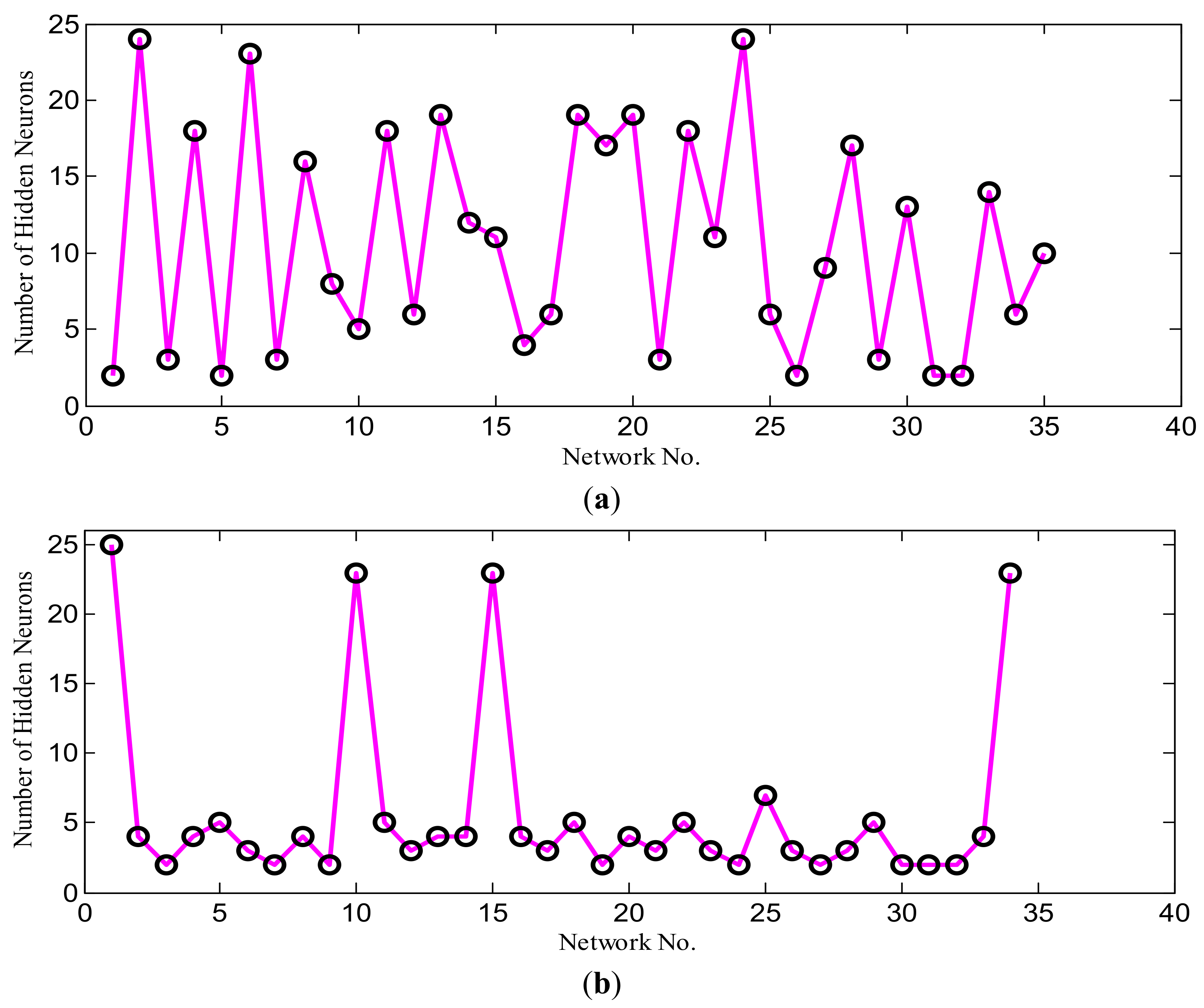
In this study, each of the developed bootstrap aggregated neural network contains 35 single hidden layer networks. The original training and testing data are put together and re-sampled via bootstrap re-sampling with replacement to generate 35 replications of the original data. Each resampled data set is then randomly partitioned into training data (70%) and testing data (30%). A single hidden layer neural network is developed on each set of resampled data. These networks are trained by utilizing the Levenberg–Marquardt training method with regularization and early stopping. The initial network weights are taken as random values uniformly distributed in the range (−0.1, 0.1), and the regularization parameter is selected as 0.1. Cross-validation is used to determine the number of hidden neurons in each individual network. In this study, 29 networks with the number of hidden neurons ranging from 2 to 30 are trained on the training data and then tested on the testing data. The network giving the smallest SSE on the testing data is considered as having the appropriate number of hidden neurons. The number of hidden neurons determined for the 35 single neural networks for sulphur and nitrogen contents are shown in Figure 5. Then, these 35 neural networks are aggregated, instead of choosing the “best” individual neural network. Finally, the combined prediction from the 35 neural networks is taken as the final model prediction [28].
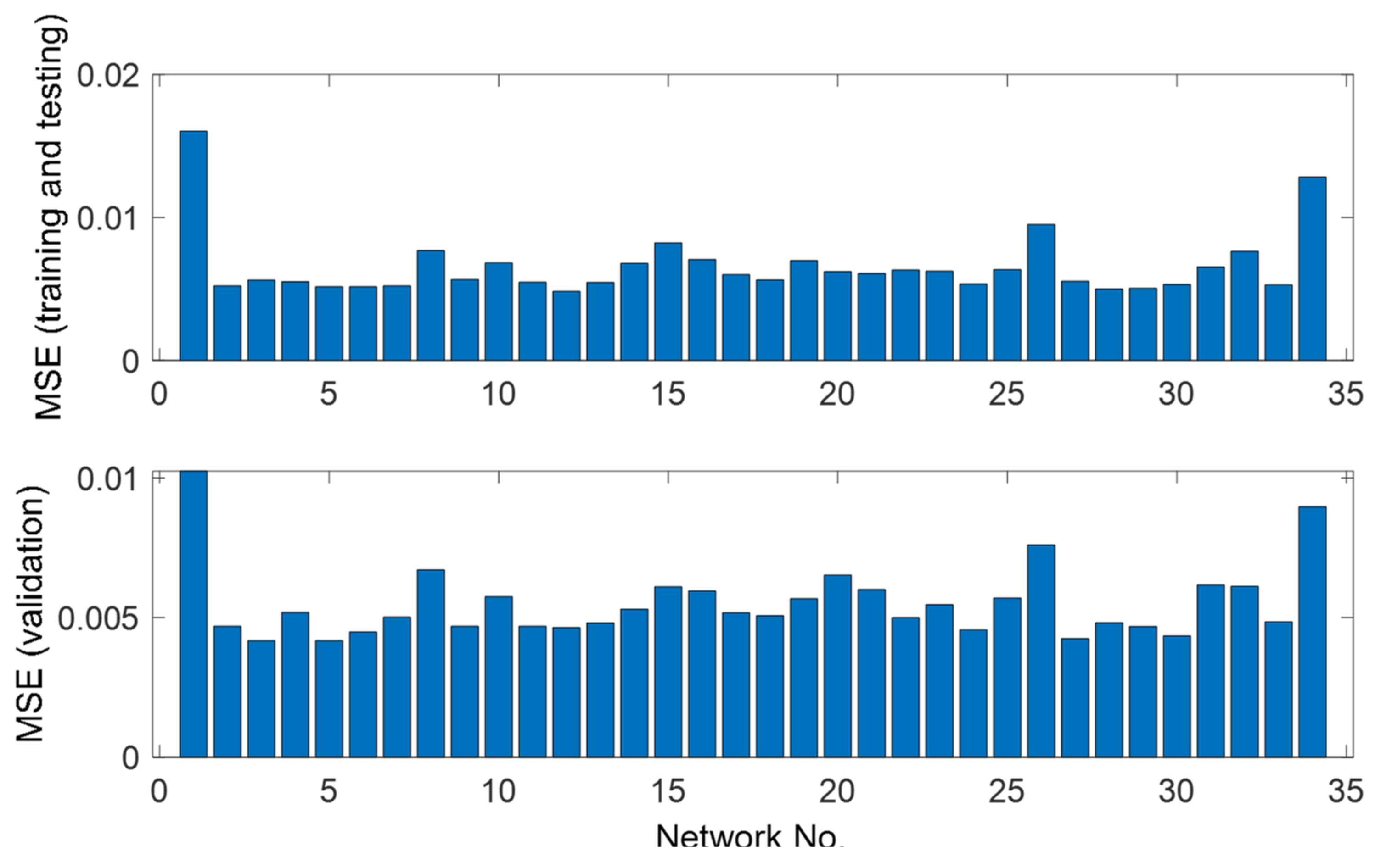
Figure 6 shows the mean squared errors (MSE) of the individual networks for predicting sulphur content on the training, testing, and unseen validation data. It can be seen that the single networks provide inconsistent performance on the training, testing, and unseen validation data. For example, the MSE on the validation data by the 12th network (0.0342) is the second largest. On the other hand, the same network gives better performance (0.0200) than many of the single networks on the training and testing data. This demonstrates that the single neural network models are not reliable.
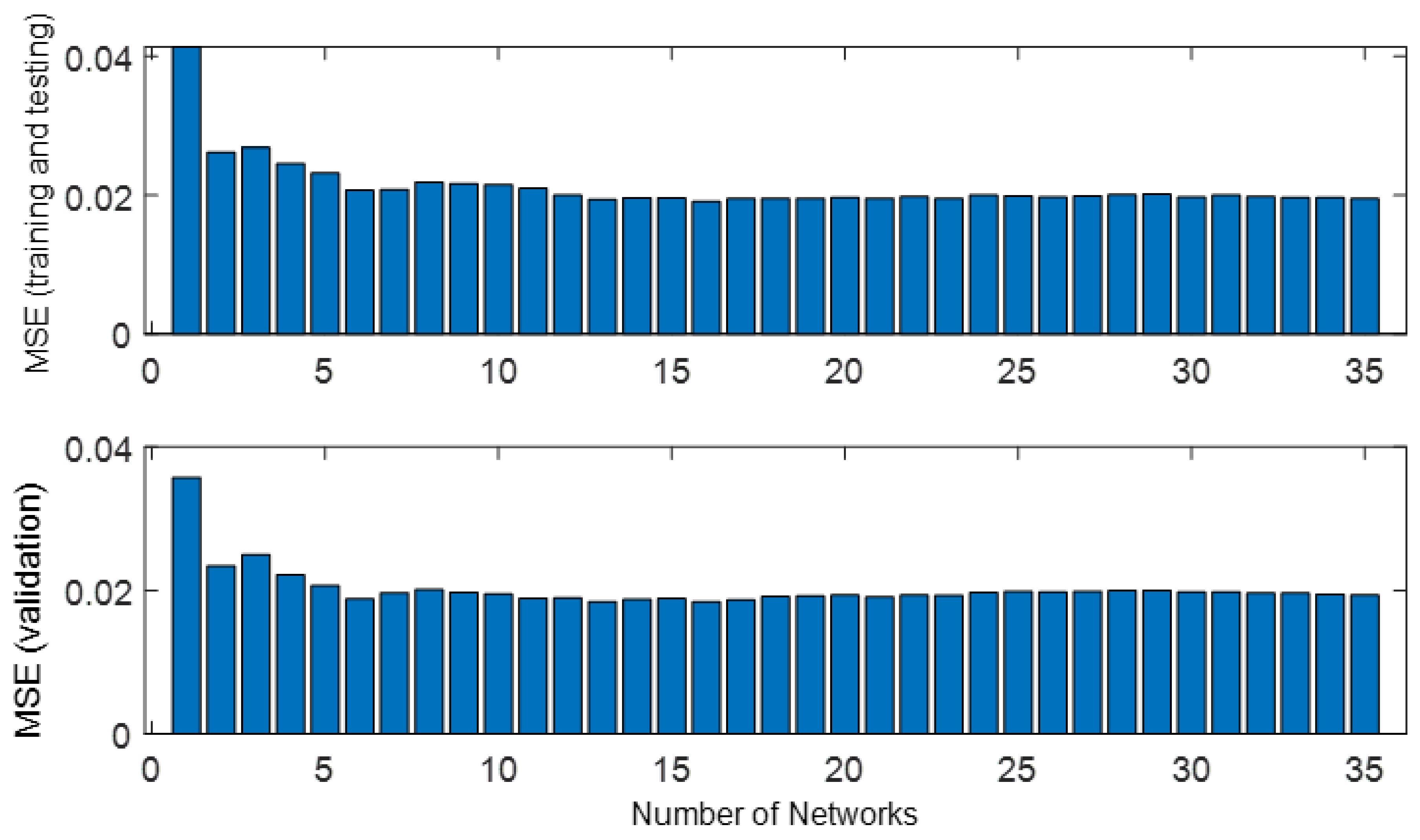
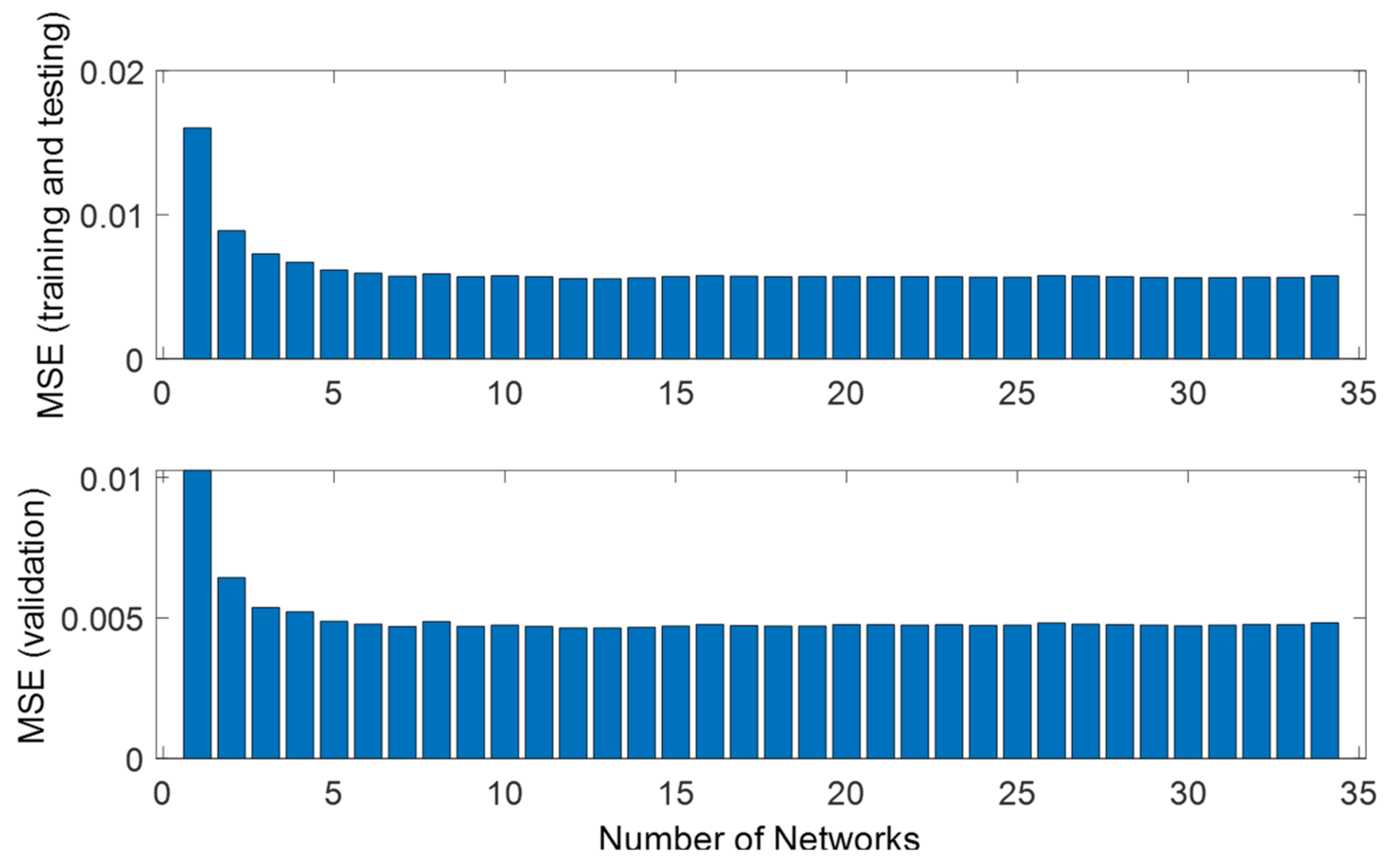
Figure 7 shows the MSE of bootstrap aggregated neural networks when stacking different numbers of networks in predicting sulphur content on the training, testing, and unseen validation data. The first bar in both plots in Figure 7 is the first single neural network shown in Figure 6, the second bar represents aggregating the first two single neural networks in Figure 6, and the last bar in Figure 7 represents aggregating all the single neural network models in Figure 6. It can be seen from Figure 7 that the MSE values on the training, testing, and unseen validation data decrease with the number of networks being aggregated and then remain stable. This clearly indicates that bootstrap aggregated neural networks are more reliable and give more accurate model prediction performance than individual neural networks.
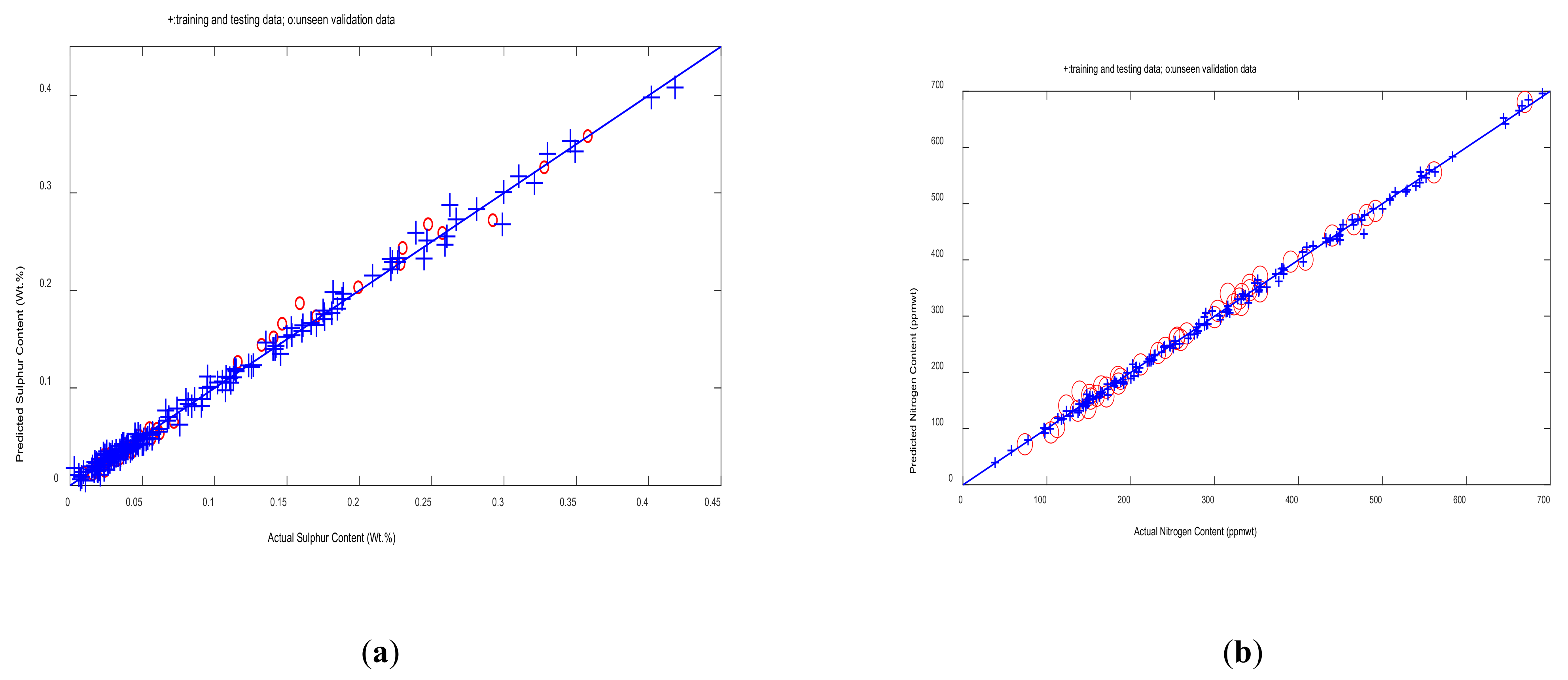
Figure 8 shows the bootstrap aggregated neural network model predictions and actual values for sulphur and nitrogen contents on the training and testing data, and the unseen validation data. The training and testing data are represented by ‘+’, and the unseen validation data are represented by ‘o’. It can be seen from both plots in Figure 8 that the model predictions correlate well with the true values for most of the samples. The bootstrap aggregated neural network model prediction performance is better than that of single neural networks shown in Figure 3. For the sulphur prediction model, there are a few samples with large errors when the sulphur content is high. This is probably due to fewer training samples in this region. However, as the optimization objective is to minimize sulphur content, the large error at the high sulphur content region has no impact on the optimization.
Figure 9 shows the MSE values of single neural networks for the prediction of nitrogen content on the training, testing, and unseen validation data. It can be seen from this figure that the 10th network gives much worse performance than any other networks on all the data sets. Thus, this network is removed. Note that the deletion of this network is purely based on its very poor performance on the training and testing data. Figure 10 shows the performance of the remaining networks. The performance of individual networks on the training and testing data is not in agreement with that on the unseen validation data. It can be seen from Figure 10 that the second network gives better performance than the third network on the training and testing data. However, its performance on the unseen validation data is worse than that of the third network. This clearly shows that the single networks are not reliable.
Figure 11 shows the MSE values of predicting nitrogen content on the training, testing, and unseen validation data by aggregating several numbers of single neural networks. In Figure 11, the first bar in both plots is the first single network in Figure 10, the second bar is aggregating the first two single networks in Figure 10, and the last bar represents aggregating all the single neural network models in Figure 10. It can be seen from Figure 11 that aggregated networks produce consistent performance on the training and testing data and on the unseen validation data. The MSE values of bootstrap aggregated neural networks decrease and remain stable on the training, testing, and unseen validation data as more networks are aggregated. Furthermore, it can be observed that bootstrap aggregated neural networks are more accurate and reliable than single neural networks. Figure 7 and Figure 11 indicate that model errors level off after combining about 10 networks. Although combining more networks does not further improve model accuracy, the estimation of model prediction confidence bounds (to be discussed in Section 3.3) would not be accurate if too few networks are used.

3.3. Neural Network Model Prediction Confidence Bounds

One major advantage with the use of bootstrap aggregated neural networks is that model prediction confidence bounds can be easily estimated from the predictions of individual neural networks [31]. Confidence bounds reveal how confident the associated prediction is.
The standard error of the individual network predictions can be estimated as:
σ e = 1 n 1 i = 1 n f i x y x 2 1 2
where n is the number of neural networks in the aggregated neural network and y x = i = 1 n f i x /n. The 95% confidence bounds for the prediction corresponding to an input x is estimated as y(x) ± 1.96 σ e . A lower   σ e , i.e., a narrower confidence bound, means that the model prediction is more reliable.
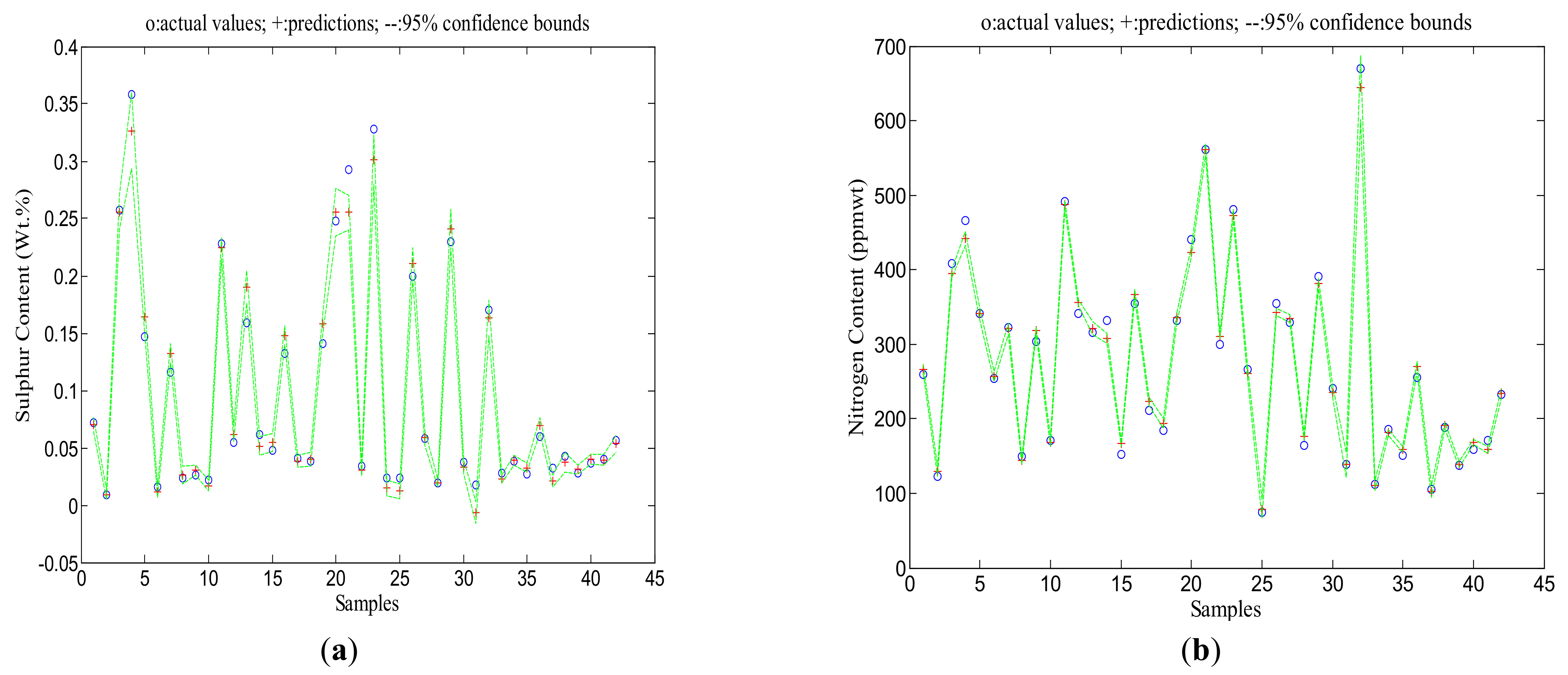
Figure 12a,b show the 95% model prediction confidence bounds for predicting sulphur and nitrogen contents on the unseen validation data by aggregated neural network models, respectively. The actual values are represented by “o”, the predicted values from the aggregated network models are represented by “+”, and 95% confidence intervals are represented by the green dashed lines. When the confidence bounds are tight, the reliability of the model predictions will be high. It can be seen that model predictions using bootstrap aggregated models are quite close to the real values for most of the samples. Furthermore, the confidence bounds are quite narrow for most of the samples indicating reliable model predictions. It can be concluded that the bootstrap aggregated neural network models for sulphur and nitrogen contents give very good performance.

4. Multi-Objective Optimization of the Process Using the Goal-Attainment Technique

Multi-objective optimization is a field of multiple criteria decision-making, which is concerned with mathematical optimization problems with conflicting objectives [33]. A single objective function in many cases with various constraints cannot adequately represent the multi-criteria decision-making problem, such as balancing results between profit and energy costs [34]. When the number of objectives rises, trade-offs become complicated. Multi-objective optimization includes minimizing or maximizing various objectives which are subject to a number of constraints. It is concerned with the creation of non-inferior solutions which are also named as efficient or Pareto optimum solutions [35]. According to a formal definition provided by [36], “a non-inferior solution is one in which no decrease can be obtained in any of the objectives without causing a simultaneous increase in at least one of the other objectives”. A non-inferior solution is also known as Pareto front or Pareto optimal.
Some common methods for multi-objective optimization include: goal-attainment, minimax, and multi-objective genetic algorithm. In this study, the multi-objective optimization problem for the crude oil hydrotreating process with the crude distillation unit is solved using the goal-attainment method.

4.1. Goal-Attainment Method

The goal-attainment method is a powerful tool which can be used to find the best solution in a multi-objective optimization problem. In this method, the decision-maker specifies a goal for each of the objectives. This method includes a set of goals F x = F 1 x ,   F 2 x ,   F 3 x , ,   F n x which are associated with a set of objectives Y x = Y 1 x ,   Y 2 x ,   Y 3 x , ,   Y n x . Also, a set of weighting factors W x = W 1 x ,   W 2 x ,   W 3 x , ,   W n x is used to control the degree of goal achievement [37]. Figure 13 shows the goal-attainment method with two objectives, Y1 and Y2.
It can be seen from Figure 13 that the goal point P is defined by goals (Y1* and Y2*) corresponding to the two objectives Y1 and Y2, respectively, while the weighting factors W determines the direction of search from the goal point P to the feasible space Ʌ(Ɣ). The set of nonlinear solutions can be obtained by changing W over Ʌ during the optimization.
In this work, the multi-objective optimization problem deals with three process operation objectives, namely, minimization of sulphur content, minimization of nitrogen content, and maximization of production rate. Four decision variables are selected and they are feedstock flow rate, H2 molar flow rate, reactor temperature, and pressure. These four decision variables are also the neural network model inputs.
The multi-objective optimization problem considered in this paper can be represented as follows:
Y = S N f
min x , γ γ s . t . Y i x W i   γ     F i       i = 1 ,   2 ,   3 L B i   x i   U B i       i = 1 ,   2 ,   3 ,   4 Equations   ( 1 )   and   ( 2 )
In the above equation, Y is a vector of the objectives, S and N are, respectively, the predicted contents of sulphur and nitrogen in the kerosene produced from the CDU, f is the crude oil feed rate, x = x 1 ,   x 2 ,   x 3 ,   x 4 is a vector of decision variables which are the neural network model inputs, LBi and Ubi are the lower and upper bounds for xi respectively and are given in Table 5, Wi is the weighting factor for the ith objective, γ is a slack variable, and Fi is the desired goal for the ith objective. The three objectives in Equation (5) are minimizing the contents of sulphur and nitrogen in the kerosene product, and maximizing the refinery throughput.
Table 6 shows two cases of the multi-objective optimization results for two sets of goals. In Case 1, the goals for sulphur content, nitrogen content, and feed flow rate were selected as 0.04 Wt.%, 140.0 ppmwt, and 70 m3/h, respectively. The weighing factors (W) were selected as 0.5, 5.0, and 0.1 for sulphur content, nitrogen content, and feed flow rate, respectively. A smaller weighting means the associated goal is more important. As can be seen from Table 6 (Case 1), all the three goals have been met according to neural network model predictions. The neural network predicted sulphur and nitrogen contents are 0.0329 Wt.% and 140.0 ppmwt, respectively. However, when the optimal process operating conditions are implemented on HYSYS simulation, the actual sulphur content decreases to 0.0300 Wt.% and the actual nitrogen content increases to 143.0 ppmwt. In Case 2, the goals for sulphur content, nitrogen content, and feed flow rate were selected as 0.03 Wt.%, 130.0 ppmwt, and 70 m3/h, respectively. The weighing factors (W) for sulphur content, nitrogen content, and feed flow rate are kept the same as those in Case 1. It can be seen from Table 6 (Case 2) that all the three goals have been met according to neural network model predictions. The neural network predicted sulphur and nitrogen contents are 0.0292 Wt.% and 130.0 ppmwt, respectively. On the other hand, when the optimal process operating conditions are implemented on HYSYS simulation, the real sulphur and nitrogen contents increase to 0.0300 Wt.% and 134.5 ppmwt, respectively.
The actual nitrogen content exceeds its goal value in both cases. This performance degradation is due to the model plant mismatch. The absolute errors shown in Table 6 are calculated as the difference between bootstrap aggregated neural network predictions and HYSYS simulation.

4.2. Reliable Multi-Objective Optimization through Incorporating Model Prediction Confidence Bounds

The reliability of optimization results is affected by the reliability of model predictions. If the model predictions are not reliable, then the optimization results based on these predictions are not likely to be reliable. Incorporating model prediction reliability in the optimization objectives could improve the reliability of optimization results. In order to improve the reliability of multi-objective optimization, minimization of the widths of model prediction confidence bounds is incorporated as additional optimization objectives. The reliable multi-objective optimization problem is given as follows:
Y = S N f C b S C b N
min x , γ γ s . t . Y i x W i   γ     F i     i = 1 ,   2 ,   3 ,   4 ,   5 L B i   x i   U B i     i = 1 ,   2 ,   3 ,   4 Equations   ( 1 )   and   ( 2 )
where Cb(S) and Cb(N) are the widths of model prediction confidence bounds for sulphur and nitrogen contents, respectively. The purpose of minimizing the width of model prediction confidence bounds is to make the model prediction more reliable leading to reliable optimization results. The goals and weights specify the relative importance of various process objectives and model prediction reliability.
Table 7 and Table 8 show the optimization results and HYSYS simulation by incorporating model prediction confidence bounds in the optimization objectives for Case 1 and Case 2, respectively. As can be seen from these tables, the goals for sulphur content, nitrogen content, and feed flow rate are kept the same as those in the corresponding cases in Table 6. Two additional goals on the widths of model prediction confidence bounds for sulphur and nitrogen contents are added here.
When solving the multi-objective optimization problem, it is expected that different optimal operating policies will be obtained from different goals and weightings. It can be seen from Table 7 (Case 1) that, as the weightings on model prediction confidence bounds are further reduced (i.e., making the model reliability more important) in run 3, model prediction reliability is improved leading to much less actual nitrogen content. The nitrogen content has been reduced from 143.0 ppmwt in all runs in Table 7 (Case 1) in the real process (HYSYS simulation). Table 8 (Case 2) shows that the weightings on model prediction confidence bounds are also further reduced in run 3 and model prediction reliability is improved leading to much fewer absolute errors between the bootstrap aggregated neural network model and HYSYS model. The nitrogen content has been reduced from 134.5 ppmwt to 127.0 ppmwt in run 3 in Table 8 (Case 2) in the real process (HYSYS simulation). This reveals the improved reliability of the proposed reliable multi-objective optimization method. As can be seen from run 3 in Table 8 (Case 2), the bootstrap aggregated neural network model predicted values for sulphur and nitrogen contents are closer to the true values compared to those in Table 6 (Case 2). It can be concluded that run 3 in Table 8 (Case 2) can be selected as the best optimum case with confidence bounds.
Table 9 compares the base case and the optimum cases of the operating conditions for HDT of crude oil with CDU. The optimal case 1 is run 3 in Table 7, while the optimal case 2 is run 3 in Table 8. It can be seen that the crude oil charge is increased significantly from 55 m3/h in the base case to about 70 m3/h in the optimum cases 1 and 2. Optimal case 2 has slightly higher sulphur and nitrogen removal than optimal case 1.

5. Conclusions

Modelling and multi-objective optimization of a crude oil hydrotreating process with a crude distillation unit using bootstrap aggregated neural networks is studied in this paper. Hydrotreating of whole crude oil is a new process with economic advantages compared to hydrotreating of individual oil products. Bootstrap aggregated neural networks are employed in this work to improve the reliability and accuracy of data-driven non-linear models. Bootstrap aggregated neural networks can also provide model prediction confidence bounds based on the individual neural network predictions. Minimization of the widths of model prediction confidence bounds is incorporated as additional optimization objectives. It is shown that reliable optimization results are obtained by incorporating model prediction confidence in the optimization objectives. The modelling and optimization results are validated using Aspen HYSYS simulation.

Author Contributions

Conceptualization, W.M. and J.Z.; methodology, W.M. and J.Z.; software, W.M. and J.Z.; validation, W.M.; formal analysis, W.M.; investigation, W.M.; resources, J.Z.; data curation, W.M. and J.Z.; writing—original draft preparation, W.M.; writing—review and editing, J.Z.; visualization, W.M.; supervision, J.Z.; and project administration, J.Z. All authors have read and agreed to the published version of the manuscript.

Funding

This research received no external funding.

Institutional Review Board Statement

Not applicable.

Informed Consent Statement

Not applicable.

Data Availability Statement

Not applicable.

Conflicts of Interest

The authors declare no conflict of interest.

References

  1. Speight, J.G. The Chemistry and Technology of Petroleum, 5th ed.; CRC Press, Taylor & Francis Group: Boca Raton, FL, USA, 2014. [Google Scholar]
  2. Gary, J.H.; Kaiser, M.J. Petroleum Refining: Technology and Economics, 5th ed.; Taylor & Francis: Boca Raton, FL, USA, 2007. [Google Scholar]
  3. Orszulik, S.T. Environmental Technology in the Oil Industry, 3rd ed.; Springer: Cham, Switzerland, 2016. [Google Scholar]
  4. Muhsin, W.A.S.; Zhang, J.; Lee, J. Modelling and optimisation of a crude oil hydrotreating process using neural networks. Chem. Eng. Trans. 2016, 52, 211–216. [Google Scholar]
  5. Rodriguez, M.A.; Ancheyta, J. Modeling of hydrodesulfurization (HDS), hydrodenitrogenation (HDN), and the hydrogenation of aromatics (HDA) in a vacuum gas oil hydrotreater. Energy Fuels 2004, 18, 789–794. [Google Scholar] [CrossRef]
  6. Jarullah, A.T.; Mujtaba, I.M.; Wood, A.S. Kinetic parameter estimation and simulation of trickle-bed reactor for hydrodesulfurization of crude oil. Chem. Eng. Sci. 2011, 66, 859–871. [Google Scholar] [CrossRef]
  7. Jarullah, A.T.; Mujtaba, I.M.; Wood, A.S. Whole crude oil hydrotreating from small-scale laboratory pilot plant to large-scale trickle-bed reactor: Analysis of operational issues through modeling. Energy Fuels 2012, 26, 629–641. [Google Scholar] [CrossRef]
  8. Muhsin, W.; Zhang, J. Modelling and optimal operation of a crude oil hydrotreating process with atmospheric distillation unit utilising stacked neural networks. In Computer Aided Chemical Engineering; Antonio Espuña, M.G., Luis, P., Eds.; Elsevier: Amsterdam, The Netherlands, 2017; pp. 2479–2484. [Google Scholar]
  9. Ancheyta, J. Modeling of Processes and Reactors for Upgrading of Heavy Petroleum; CRC Press, Taylor & Francis Group: Boca Raton, FL, USA, 2013. [Google Scholar]
  10. Shang, C.; Yang, F.; Huang, D.; Lyu, W. Data-driven soft sensor development based on deep learning technique. J. Process Control 2014, 24, 223–233. [Google Scholar] [CrossRef]
  11. Chang, H.; Su, Z.; Lu, S.; Zhang, G. Application of deep learning network in bumper warpage quality improvement. Processes 2022, 10, 1006. [Google Scholar] [CrossRef]
  12. Li, F.; Zhang, J.; Shang, C.; Huang, D.; Oko, E.; Wang, M. Modelling of a post-combustion CO2 capture process using deep belief network. Appl. Therm. Eng. 2018, 130, 997–1003. [Google Scholar] [CrossRef] [Green Version]
  13. Zhu, C.; Zhang, J. Developing soft sensors for polymer melt index in an industrial polymerization process using deep belief networks. Int. J. Autom. Comput. 2020, 17, 44–54. [Google Scholar] [CrossRef] [Green Version]
  14. Chen, B.; Huang, P.; Zhou, J.; Li, M. An enhanced stacking ensemble method for granule moisture prediction in fluidized bed granulation. Processes 2022, 10, 725. [Google Scholar] [CrossRef]
  15. Ibrahim, D.; Jobson, M.; Li, J.; Guillén-Gosálbez, G. Optimization-based design of crude oil distillation units using surrogate column models and a support vector machine. Chem. Eng. Res. Des. 2018, 134, 212–225. [Google Scholar] [CrossRef] [Green Version]
  16. Brambilla, A.; Vaccari, M.; Pannocchia, G. Analytical RTO for a critical distillation process based on offline rigorous simulation. In Proceedings of the 13th IFAC Symposium on Dynamics and Control of Process Systems, Including Biosystems (DYCOPS), Busan, Korea, 14–17 June 2022. [Google Scholar]
  17. Aspen Technology. Assay Management in Aspen HYSYS®Petroleum Refining; Aspen Technology: Houston, TX, USA, 2015. [Google Scholar]
  18. Aspen Technology. Kirkuk Crude Oil Assay; Assay Library: Houston, TX, USA, 2011. [Google Scholar]
  19. Fahim, M.A.; Alsahhaf, T.A.; Elkilani, A. Refinery feedstocks and products. In Fundamentals of Petroleum Refining; Elsevier: Amsterdam, The Netherlands, 2010; pp. 11–31. [Google Scholar]
  20. Thrampoulidis, E.; Mavromatidis, G.; Lucchi, A.; Orehounig, K. A machine learning-based surrogate model to approximate optimal building retrofit solutions. Appl. Energy 2021, 281, 116024. [Google Scholar] [CrossRef]
  21. Vaccari, M.; Pannocchia, G.; Tognotti, L.; Paci, M.; Bonciani, R. A rigorous simulation model of geothermal power plants for emission control. Appl. Energy 2020, 263, 114563. [Google Scholar] [CrossRef]
  22. Cybenko, G. Approximation by superpositions of a sigmoidal function. Math. Control Signals Syst. 1989, 2, 303–314. [Google Scholar] [CrossRef]
  23. Herrera, F.; Zhang, J. Optimal control of batch processes using particle swam optimisation with stacked neural network models. Comput. Chem. Eng. 2009, 33, 1593–1601. [Google Scholar] [CrossRef]
  24. Bishop, C. Improving the generalization properties of radial basis function neural networks. Neural Comput. 1991, 3, 579–588. [Google Scholar] [CrossRef] [PubMed]
  25. MacKay, D.J.C. Bayesian interpolation. Neural Comput. 1992, 4, 415–447. [Google Scholar] [CrossRef]
  26. Wolpert, D.H. Stacked generalization. Neural Netw. 1992, 5, 241–259. [Google Scholar] [CrossRef]
  27. Sridhar, D.V.; Seagrave, R.C.; Bartlett, E.B. Process modeling using stacked neural networks. AIChE J. 1996, 42, 2529–2539. [Google Scholar] [CrossRef] [Green Version]
  28. Zhang, J.; Martin, E.B.; Morris, A.J.; Kiparissides, C. Inferential estimation of polymer quality using stacked neural networks. Comput. Chem. Eng. 1997, 21, S1025–S1030. [Google Scholar] [CrossRef]
  29. Zhang, J. Batch-to-batch optimal control of a batch polymerisation process based on stacked neural network models. Chem. Eng. Sci. 2008, 63, 1273–1281. [Google Scholar] [CrossRef]
  30. Khaouane, L.; Ammi, Y.; Hanini, S. Modeling the retention of organic compounds by nanofiltration and reverse osmosis membranes using bootstrap aggregated neural networks. Arab. J. Sci. Eng. 2017, 42, 1443–1453. [Google Scholar] [CrossRef]
  31. Zhang, J. Developing robust non-linear models through bootstrap aggregated neural networks. Neurocomputing 1999, 25, 93–113. [Google Scholar] [CrossRef]
  32. Li, F.; Zhang, J.; Oko, E.; Wang, M. Modelling of a post-combustion CO2 capture process using extreme learning machine. Int. J. Coal Sci. Technol. 2017, 4, 33–40. [Google Scholar] [CrossRef] [Green Version]
  33. Koziel, S.; Bekasiewicz, A. Multi-Objective Design of Antennas Using Surrogate Models; World Scientific: Singapore, 2016. [Google Scholar]
  34. Vaccari, M.; Capaci, R.B.; Brunazzi, E.; Tognotti, L.; Pierno, P.; Vagheggi, R.; Pannocchia, G. Optimally Managing Chemical Plant Operations: An Example Oriented by Industry 4.0 Paradigms. Ind. Eng. Chem. Res. 2021, 60, 7853–7867. [Google Scholar] [CrossRef]
  35. Miettinen, K. Nonlinear Multiobjective Optimization; Kluwer Academic Publishers: Boston, MA, USA, 1998. [Google Scholar]
  36. Haimes, Y.Y.; Hall, W.A.; Freedman, H.T. Multiobjective Optimization in Water Resources Systems: The Surrogate Worth Trade-off Method; Elsevier: Amsterdam, The Netherlands, 2011. [Google Scholar]
  37. Osuolale, F.N.; Zhang, J. Multi-objective optimisation of atmospheric crude distillation system operations based on bootstrap aggregated neural network models. Comput. Aided Chem. Eng. 2015, 37, 671–676. [Google Scholar]
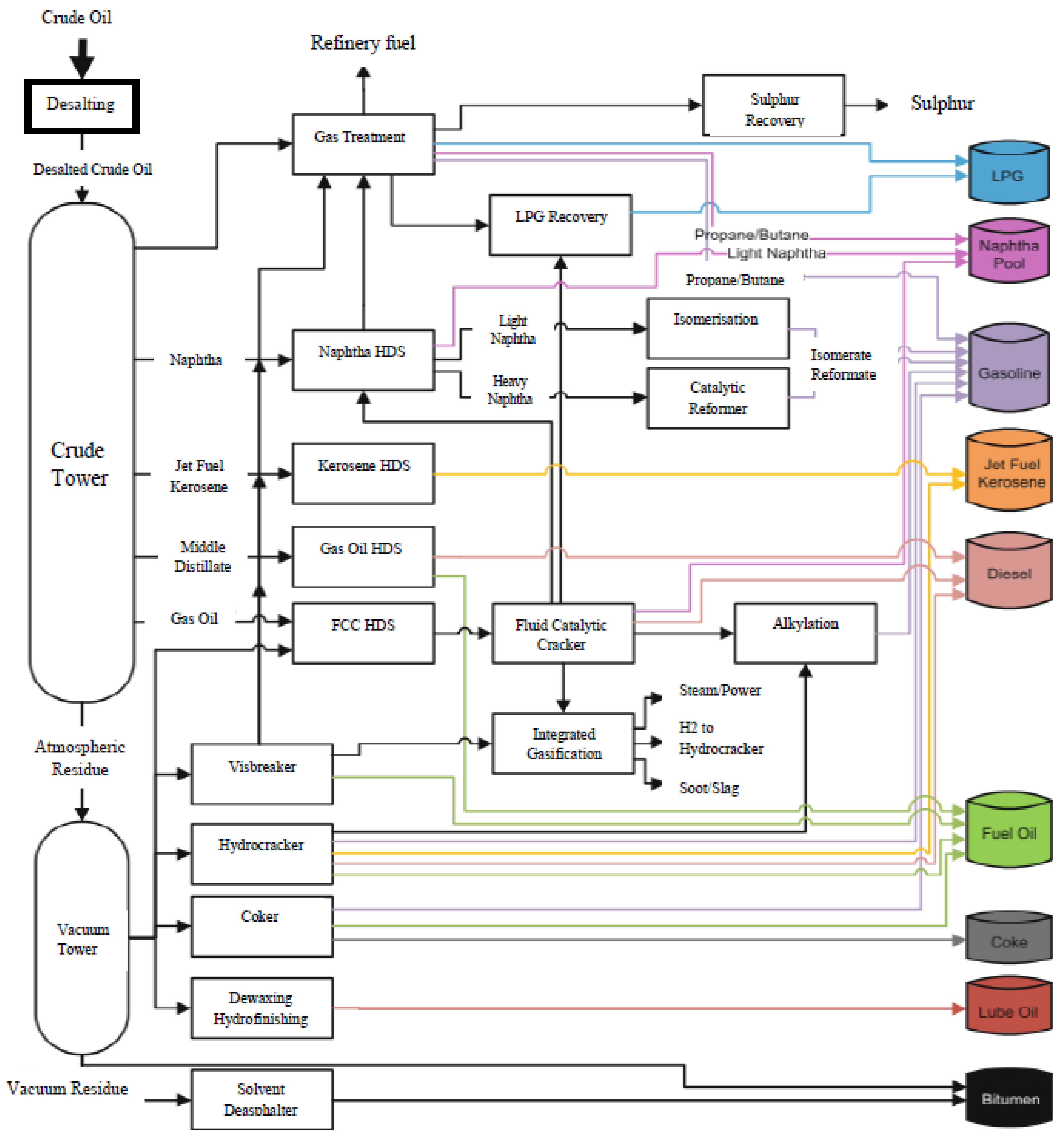
Figure 1. Flow sheet diagram of a crude oil refinery.
Processes 10 01438 g001
Figure 2. HDT for crude oil with CDU.
Processes 10 01438 g002
Figure 3. Network model performance on the training, testing, and validation data for sulphur content (a) and nitrogen content (b).
Processes 10 01438 g003
Figure 4. A bootstrap aggregated neural network.
Processes 10 01438 g004
Figure 5. Number of hidden neurons of single neural networks for sulphur content (a) and nitrogen content (b).
Processes 10 01438 g005
Figure 6. Errors of signal neural networks for estimating sulphur content.
Processes 10 01438 g006
Figure 7. Errors of stacked neural networks for estimating sulphur content.
Processes 10 01438 g007
Figure 8. Stacked networks prediction and real values for sulphur content (a) and nitrogen content (b).
Processes 10 01438 g008
Figure 9. Errors of signal neural networks for estimating nitrogen content (35 networks).
Processes 10 01438 g009
Figure 10. Errors of signal neural networks for estimating nitrogen content (34 networks).
Processes 10 01438 g010
Figure 11. Errors of stacked neural networks for estimating nitrogen content.
Processes 10 01438 g011
Figure 12. Stacked neural network predictions of sulphur content (a) and nitrogen content (b) on the unseen validation data.
Processes 10 01438 g012
Figure 13. The goal-attainment method for a two-dimensional problem.
Processes 10 01438 g013
Table 1. Operating conditions of various HDT processes [9].
Hydrotreating ProcessT (°C)PH2 (MPa)LHSV (h−1)H2/Oil (Nm3/m3)
Naphtha3201–23–860
Kerosene3302–32–580
Gasoil3402.5–41.5–4140
VGO3605–91–2210
Atmospheric Residue370–4108–130.2–0.5˃525
Hydrocracking VGO380–4309–200.5–1.51000–2000
Vacuum Residue400–44012–210.1–0.51000–2000
Table 2. Petroleum Essay.
No.PropertyBulk Value
1Sulphur By (Wt.%)2.63
2Std Liquid Density (kg/m3)867.5162
3Watson K11.4279
4Pour Point (°C)21.8696
5Total Acid Number (mg KOH/g)0.171
6Kinematic Viscosity (cSt)@ 20 (°C)13.0798
7Kinematic Viscosity (cSt)@ 37.78 (°C)7.7831
8Kinematic Viscosity (cSt)@ 37.78 (°C)7.7831
9Kinematic Viscosity (cSt)@ 50 (°C)5.697
10Kinematic Viscosity (cSt)@ 60 (°C)4.5238
11Kinematic Viscosity (cSt)@ 80 (°C)2.9883
12Kinematic Viscosity (cSt)@ 100 (°C)2.0967
13NaCl By (Wt.%)0.002
14Mercaptan Sulphur By (Wt.%)0.0217
15Conradson Carbon By (Wt.%)6.0699
16Asphaltene By (Wt.%)2.3412
17Nickel By (Wt.%)0.0008
18Vanadium By (Wt.%)0.0037
19Iron By (Wt.%)0.0001
20Gross Heating Value (kJ/kg)44,157.58
21Net Heating Value (kJ/kg)41,482.25
22Cut Yield By (Wt.%)100
23Cut Yield By (Vol.%)100
24Nitrogen By (Wt.%)0.1113
25Paraffins By (Vol.%)30.5540
26Naphthenes By (Vol.%)40.8213
27Arom By (Vol.%)28.6245
28N + 2A (%)98.0705
29Smoke Pt (m)0.0156
30Freeze Point (°C)79.3312
31Basic Nitrogen By (Wt.%)0.0378
32Cloud Point (°C)38.6010
33CtoH Ratio By Wt6.6651
Table 3. Crude distillation products.
Cut
Oils
Yield
(Wt.%)
Specific Gravity at 15 °CFlash Point (°C)ColorTBP
(°C)
Fuel gases0.01
LPG0.12
LN8.980.665–0.68035–120
HN12.400.735–0.75090–178
Ker10.800.785–0.80040 min.30 min.135–250
LGO17.700.825–0.84070 min.0.5 max.200–350
HGO3.680.880–0.89090 min.2.5 max.335–355
RC46.310.965–0.980120 min.355+
Table 4. Crude oil hydrocarbon ranges.
Petroleum ProductsCarbon Range
Fuel gases C1–C2
LPGC3–C4
LN and HNC5–C12
KerC12–C16
LGO and HGOC12–C20
Lubricating oilC20–C50
RC>C50
Table 5. The lower and upper bounds of the process operation variables.
VariablesUnitsLower BoundsUpper Bounds
crude oil flow ratem3/h4070
hydrogen flow ratekgmole/h7001000
reactor pressurebar70130
reactor temperature°C330380
Table 6. Multi-objective optimization results without confidence bounds.
CaseGoalsCb(S)Cb(N)WxStacked NetworkHYSYSAbsolute Error
1 0.04 140 70 0.01770.0149 0.5 5 0.1 70 802.66 123.89 377.68 S: 0.0329
N: 140.0000
S: 0.0300
N: 143.0000
0.0029
3.0000
2 0.03 130 70 0.01680.0171 0.5 5 0.1 70 802.83 125.99 377.60 S: 0.0292
N: 130.0000
S: 0.0300
N: 134.5000
0.0008
4.5000
Table 7. Multi-objective optimization results with confidence bounds (Case 1).
RunGoalsWxStacked NetworkHYSYSAbsolute Error
1 0.04 140 70 0.01 0.01 0.5 5.0 0.1 1.0 1.0 69.9993 802.86 126.37 377.18 S: 0.0294
N: 132.6498
Cb(S): 0.0165
Cb(N): 0.0165
S: 0.0300
N: 137.7000
0.0006
5.0502
2 0.04 140 70 0.01 0.01 0.5 5.0 0.1 0.5 0.5 69.9987 802.86 126.37 377.18 S: 0.0294
N: 132.6510
Cb(S): 0.0165
Cb(N): 0.0165
S: 0.0300
N: 137.7000
0.0006
5.0490
3 0.04 140 70 0.01 0.01 0.5 5.0 0.1 0.05 0.05 69.9922 861.56 120.88 376.90 S: 0.0322
N: 139.5789
Cb(S): 0.0139
Cb(N): 0.0139
S: 0.0300
N: 132.6000
0.0022
6.9789
Table 8. Multi-objective optimization results with confidence bounds (Case 2).
RunGoalsWxStacked NetworkHYSYSAbsolute Error
1 0.03 130 70 0.01 0.01 0.5 5.0 0.1 1.0 1.0 69.9993 802.81 125.70 377.74 S: 0.0294
N: 132.0352
Cb(S): 0.0170
Cb(N): 0.0170
S: 0.0300
N: 134.1000
0.0006
4.0648
2 0.03 130 70 0.01 0.01 0.5 5.0 0.1 0.5 0.5 69.9986 802.81 125.70 377.74 S: 0.0294
N: 130.0704
Cb(S): 0.0170
Cb(N): 0.0170
S: 0.0300
N: 137.7000
0.0006
4.0296
3 0.03 130 70 0.01 0.01 0.5 5.0 0.1 0.05 0.05 69.9878 836.62 122.27 378.00 S: 0.0304
N: 130.6100
Cb(S): 0.0160
Cb(N): 0.0160
S: 0.0300
N: 127.0000
0.0004
3.6100
Table 9. Comparison of the base case and the optimum cases.
CasesFeed
(m3/h)
H2 Molar Flow (kgmole/h)Pressure
(bar)
Temperature
(°C)
S Removal (Wt.%)N Removal (Wt.%)
Base55.00800.0090.00375.0085.3288.08
Optimum 169.65865.01120.78376.4288.6388.18
Optimum 269.99836.62122.27378.0088.6488.63
Publisher’s Note: MDPI stays neutral with regard to jurisdictional claims in published maps and institutional affiliations.