Abstract
Temperature and its distribution are crucial for combustion monitoring and control. For this application, digital camera-based pyrometers become increasingly popular, due to its relatively low cost. However, these pyrometers are not universally applicable due to the dependence of calibration. Compared with pyrometers, monitoring cameras exist in all most every combustion chamber. Although these cameras, theologically, have the ability to measure temperature, due to lack of calibration they are only used for visualization to support the decisions of operators. Almost all existing calibration methods are laboratory-based, and hence cannot calibrate a camera in operation. This paper proposes an online calibration method. It uses a pre-calibrated camera as a standard pyrometer to calibrate another camera in operation. The calibration is based on a photo taken by the pyrometry-camera at a position close to the camera in operation. Since the calibration does not affect the use of the camera in operation, it sharply reduces the cost and difficulty of pyrometer calibration. In this paper, a procedure of online calibration is proposed, and the advice about how to set camera parameters is given. Besides, the radio pyrometry is revised for a wider temperature range. The online calibration algorithm is developed based on two assumptions for images of the same flame taken in proximity: (1) there are common regions between the two images taken at close position; (2) there are some constant characteristic temperatures between the two-dimensional temperature distributions of the same flame taken from different angles. And those two assumptions are verified in a real industrial plants. Based on these two verified features, a temperature distribution matching algorithm is developed to calibrate pyrometers online. This method was tested and validated in an industrial-scale municipal solid waste incinerator. The accuracy of the calibrated pyrometer is sufficient for flame monitoring and control.
1. Introduction
Combustion may be found in a wide range of industrial processes, such as thermal power generation, and metallurgy processes [1], where combustion is closely associated with pollution emission and energy consumption. For environmental protection and energy saving, efficient and precise combustion control and monitoring become increasingly important [2].
In current practice, most combustion control and monitoring technologies are based on the analysis of flue gases. Nevertheless, measurement provided by a flue gas analyser might be neither sufficient nor in time to indicate an abnormal state of a combustion process [2,3], because the flue gas analyser and the combustion chamber are distantly separated in most industrial processes. As a result, it is obviously insufficient to take action on burner settings to optimize the combustion processes only based on the information supplied by flue gas analysers.
This situation could be improved if the flame temperature and distribution could be used for combustion control and monitoring [4].
Digital flame imaging has been historically an invaluable technology in combustion monitoring since it provides spatial status of the flames. During past decades, many advanced flame imaging devices have been developed for temperature distribution measurement. These are mainly divided into two categories: active imaging technologies (also called laser-based technologies) [5,6] and passive imaging technologies [7,8,9]. Due to the high cost and difficulty to set up, the former are almost only applied to laboratorial systems [2]. By contrast, the latter receive more attention in industry, because they could achieve high temporal and spatial resolution at a reasonable cost by employing conventional digital cameras [2,3].
Nowadays, video cameras could be found in almost all industrial combustion facilities. They are, however, only utilized for online display on control room monitors. The operator subjectively analyses the flame image based on previous experience to identify the combustion state [10]. Theoretically, it is possible to convert a video camera to a pyrometer after a proper calibration. However, such a pyrometer is still not widely adopted in industry. Currently, with the development of machine learning and image processing technologies, more and more research attentions are attracted on how to monitor the combustion state with the deep information of the flame image [11,12,13,14]. The features extracted by machine learning methods can help to better understand the state of the current operating process and they can be used in close-loop control [15]. However, those methods treated the combustion process as a black box resulting in that the performance of the monitoring model mainly depends on the scale and quality of the labelled data [16], and have no clear physical meaning. If the domain knowledge and the physical principles can be integrated in machine learning, it would improve the model performance and generalization [17,18]. Compared with raw image data, temperature and its distribution are easier to link with domain knowledge and physical principles. Therefore, if the flame temperature distribution could be measured, performance of combustion monitoring and control would be significantly improved.
Calibration is one of the biggest challenges to equip digital cameras with pyrometry [19], because the parameters of digital camera-based temperature measurement model are closely related to the inherent attributes of cameras. There are two classes of commonly used calibration methods at present:
- 1.
- Indirect methods: camera spectral response calibration
- 2.
- Direct methods: estimating model parameters with reference temperature
The indirect methods focus on estimating camera spectral response curve. The most common approach in this category is the radiometric self-calibration based on High Dynamic Range (HDR) imaging [20]. In this method, the exposure setting of the camera to be calibrated is gradually increased resulting in a spectrum of images from underexposed to saturated. However, the video cameras used in industries might not be set exposure freely.
For the direct methods, Equation (1) represents the general direct calibration process.
where is the reference temperature and represents the temperature measurement model. is the model parameter and is the sensor output signal which is used to measure temperature. As shown in Equation (1), the calibration is a process of estimating unknown parameters in the temperature measurement model by comparing estimated temperature with reference temperature. The reference temperature is usually supplied by the blackbody furnace [21]. That means the calibration experiment must be done in advance in a laboratory.
In summary, employing those existing methods, a specific series of photos have to be taken for calibration, which are either the same picture with different camera parameters, or a series of blackbody furnace radiation pictures for the target temperature range. That means that the camera could not be used for online monitoring during the calibration process. Moreover, if the existing video camera is replaced with a calibrated camera, although the temperature distribution could be measured, the operational knowledge based on the original camera image may become invalid, because the flame images in colours, shapes and positions captured by different cameras may not be the same. For not fully automated combustion processes, such operational knowledges are essential for daily operation. Using a new camera may significantly affect normal operation. Besides, it is difficult to add one optical access to combustion chamber for the camera in a practical device. Indeed, windows and window mounts have to withstand flow’s pressure and temperature in the chamber. Film cooling using purge gas may also be required for in-situ measurements to cool the windows and prevent soot and particles from striking and depositing on the surface. Although future combustors may be designed to have optical access components, retrofitting existing systems still need clever engineering [3]. As a result, it will be desirable if the calibration could be accomplished online. Consistently, it will improve the performance of combustion control and monitoring in a very convenient and inexpensive way.
In this paper, a procedure for on-line calibration of a video camera in operation with a pre-calibrated pyrometer is proposed. Because the pre-calibrated pyrometer and the video camera take flame images at different locations, angles and times, whilst industrial flames are always flickering, it is difficult to find a common region in flame images taken by the two cameras. To solve this problem, in this paper, an on-line calibration algorithm based on flame temperature distribution matching is developed. The calibration procedure and the algorithm are tested in an industrial-scale municipal solid waste incinerator (MSWI).
This paper focuses on how to calibrate the digital camera in use for pyrometry. The main contributions are as follows:
- 1.
- An experimental procedure for online pyrometry calibration of the camera in use is proposed.
- 2.
- Experimentally, it is found that there are two peaks in the flame temperature distribution, and the temperature corresponding to the peak remains unchanged in a short period. Based on this phenomenon, a digital camera-based pyrometry calibration algorithm is developed.
- 3.
- The procedure and algorithm are tested in an industrial-scale MSWI. The calibration was successfully completed without affecting normal operation of the plant. The calibrated pyrometer meets the accuracy requirements of combustion control and monitoring.
The remainder of this paper is organized as follows. Section 2 reviews the principle of radiation thermometry and pyrometry based on digital camera. The procedure of the online calibration is then proposed in Section 3. In Section 4, the details of the calibration algorithm are given. A real calibration case study is reported in Section 5. Finally, this work is summarised in Section 6.
2. Digital Camera-Based Pyrometry Model
2.1. Principle of Thermal Radiation Temperature Measurement
According to Planck’s Law [22], the radiation intensity of a grey body object at wavelength per unit area per unit wavelength is:
where h is the Planck’s constant, c is the speed of light, k is the Boltzmann constant, T is the grey body object temperature and is the object emissivity.
If the object wavelength is within the range of 300 nm to 1000 nm and the object temperature T is between 800 k to 2000 k, . Then, Planck’s Law can be simplified to Wien’s Law [22]:
2.2. Digital Camera-Based Pyrometry
In order to capture colourful image, the colour filters are configured in the front of image sensors. The digital cameras use red, green and blue filters at the same time. The camera image sensor model can be expressed as [20]:
where and B stand for the Red, Green and Blue channels, is the intensity of sensor response, is the amplification factor of sensor and spectral response factor. Applying mean value theorems for definite integrals to Equation (4), it can be simplified to:
where is a constant between 380 nm to 780 nm.
And substituting Equation (3) into Equation (5) and taking the logarithm yields:
where let and to simplify the expression. and are the pyrometry model parameters. According to [21], if the emissivity is wavelength independent at the known temperature, the radio pyrometry can yield better result. It is reasonable to set [23]. Besides, two-colour pyrometry is less sensitive to noise than other higher radio methods [21]. Applying the radio pyrometry, Equation (5) is changed into:
where r is defined as the ratio of R channel radiation intensity to G channel radiation intensity, and taking the logarithm on both sides of Equation (7) yields:
and are the radio pyrometry model’s parameters, and express Equation (8) in matrix form:
where is a vector of the ground-true temperatures of the samples. is the parameter of this pyrometry model, and is the optimal parameter. Each element in is
where the subscript j denotes the j-th sample.
If the temperature of N pixels is known, the calibration process can be formulated as
And the closed-form solution of Equation (11) is
2.3. Revision of Radio Pyrometry
Combining Equations (8) and (5), it can be seen that the parameters of the radio pyrometry model are affected by temperature, so the traditional radio pyrometry is only effective within a certain temperature range.
In the light of Equation (5), under the same radiation intensity, the intensity of sensor response is determined as long as the temperature is determined. In another word, is a function of T or . And the traditional radio pyrometry ignores the change of caused by temperature change, resulting from which the radio pyrometry is only satisfied in a narrow temperature range. Even after calibration, it is difficult to ensure high accuracy of temperature measurement at a large temperature range. However, the temperature range of flames is always wide in some large combustion processes, such as the municipal solid waste incineration process.
According to Equation (8), is a function of , and can be considered as a function of . So and can be treated as functions of . Based on this, a Taylor expansion of Equation (8) around gives:
where is a nominal point of r. and stand for the first derivative of and with respect to . So can be approximately expressed as a quadratic function about the logarithm of image sensor response intensity . , and are the parameters of this quadratic function. Here, the matrix form of the revised radio pyrometry is
and Equations (13) and (14) are the revisions of radio pyrometry, they can be used in a wide range of temperature. Their calibration process and their closed-form solution can still be expressed by Equations (11) and (12).
3. Procedure of Online Pyrometer Calibration
The procedure of online pyrometer calibration is shown in Figure 1. The calibration process is generally divided into two parts: offline preparation and online experiment. Offline preparation is to calibrate a digital camera for pyrometry in labs using traditional approaches. The online experiment is to take photo at the viewing port around the video camera using the pre-calibrated camera, and then the online calibration algorithm is executed to estimate the parameters of the pyrometry model. Indeed, it is necessary to select camera parameters during the offline calibration, and appropriate camera parameters would improve temperature measurement accuracy. So in this section, firstly, advice is given on setting camera parameters via reviewing the physical model of the camera sensor, and the procedure of online pyrometer calibration will be described in detail next.
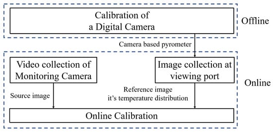
Figure 1.
Procedure of online calibration.
3.1. Physical Model of Camera Sensor
Figure 2 depicts four cells of a conventional camera sensor array. The sensor converts an instant, time-varying light field to electric charge , which is stored in cell . Formulate this process:
where is the aperture time of the camera and denotes the region of cell . It is worth noting that each sensor of the camera has only one filter, either R or G or B. RGB colour filters are arranged particularly in digital cameras. Figure 2 is one of the filter patterns called RGGB. In order to get the colour of each pixel, demosaicing needs to be done, which interpolates the colour value of the pixels of the same colour in the neighbourhood. Take pixel as an example:

Figure 2.
Camera sensor array.
For flame imaging, the light field can be expressed as Equation (3). And the traditional radio pyrometry considers that the light field remains unchanged during 0 to , and because the single sensor of the digital camera is very small, the spatial variation of light field could be also ignored. Thus, Equation (15) is simplified into:
where denotes the area of a single camera sensor and is the light field at . Because and are constant,
Because of this simplification, the shorter is and the smaller is, the more accurate the pyrometer will be. Therefore, setting the maximum shutter speed and choosing a high-resolution camera can obtain relatively higher accuracy for temperature measurement.
Furthermore, high ISO (camera’s sensitivity to light) usually introduce noise into the image, so setting a smaller ISO is better.
3.2. Offline Calibration of Digital Camera for Pyrometry
As shown in Equation (1), the calibration is a process of estimating unknown parameters in the temperature measurement model by comparing the estimated temperature with a certain ground-true temperature. The blackbody furnace can provide the reference temperature [21]. The photos should be shot in manual mode. The high shutter speed and small ISO should be setted according to the advice proposed in Section 3.1. Finally, the appropriate aperture size is setted to get sharp images without exposure. The reference temperature is then provided by the blackbody furnace. After that we need to set the blackbody furnace at different temperatures, and use the camera to take pictures of the blackbody at each temperature. The temperature range of the blackbody furnace should cover the potential application range. The calibration can be completed by Equation (12).
3.3. Online Calibration Setup of Digital Camera for Pyrometry
Currently, video cameras have already been installed in all most every large combustion equipments, and meanwhile, they usually have some viewing ports for human to watch combustion chamber directly. And some of those ports are physically close to the position of video cameras as a backup in case the cameras fail. So it makes sense that there are common regions between the visual fields of the video camera and those of viewing ports. That means the images taken at the viewing port have the common region with the frame captured by the video camera. Figure 3a illustrates the sketch of this scenario. So the flame temperature distribution measured via taking images at these viewing ports using a pre-calibrated pyrometer can be used to calibrate the video camera as long as the measured temperature can correspond to the video frame.
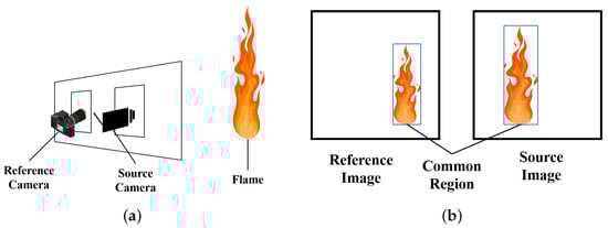
Figure 3.
The sketch of online calibration of digital camera for pyrometry. (a) Reference Camera and Source Camera; (b) Reference Image and Source Image.
Figure 3a illustrates the scenario of the online calibration experiment. For the sake of convenience, the combustion monitoring video camera in use is referred to as the Source Camera, and the image captured by this camera is referred to as the Source Image. The image-based pyrometer (pre-calibrated camera for pyrometry) is called Reference Camera, and the image taken by this pyrometer is called Reference Image.
Usually, there will be a viewing port near the video camera for the operator to directly observe the flame. Therefore, as shown in Figure 3b, if flames are shot from the viewing port with the reference camera, it makes sense to assume that the source image has a certain common region with the reference image and the common region represents the same part of flame. Next section introduces the online calibration algorithm to obtain temperature measurement model parameters.
4. Online Pyrometer Calibration Algorithm Based on Flame Temperature Distribution Matching
As Figure 3b shows, there is a common region between the reference image and the source image, and the common region represents the same part of flame.
However, the reference image and the source image are taken from different positions, different angles and by using different cameras. As depicted in Figure 4, those two images need to be transformed into a same coordinate to align those images. The image registration technology is used to accomplish this task. If the images have enough salient structures–features [24], such as the corner point, this task will be solved more easily and efficiently.

Figure 4.
The sketch of online calibration of digital camera for pyrometry.
However, the source image is full of flame in a real industrial plant. What’s worse, burning gases or vaporized fuel are always in turbulent flows, which makes the flame never be stable. Thus, even for flames captured at same times and same place, the difference between the two images could be very large. Besides, the resolutions of source camera and reference camera may differ by 1–2 orders of magnitude and the source camera may not be given a tune-up with colour balance adjustment. For example, the same object appears red in the source image but yellow in the reference image. All in all, the image registration technology may not work well in this scenario. Despite this, there are still some special zones of flame with characteristic temperature in a short time. If those areas can be detected in the source and reference images separately, the calibration can be also accomplished.
4.1. Flame Temperature Distribution and Flame Zones
As shown in Figure 5, according to flame colour, the flame can usually be divided into several parts. There exist two interesting characteristics between flame temperature distribution and flame zones:
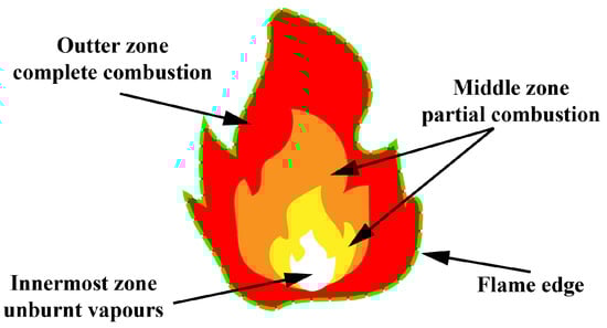
Figure 5.
Structure of flame.
- 1.
- The innermost zone of flame is the unburnt vapours, this zone is the coldest. The temperature of this zone is relatively consistent at similar combustion condition. According to flame reaction kinetics [25,26], the unburnt vapours temperature range is narrow.
- 2.
- The edge of the flame is the hottest zone of the flame, and the highest temperature of a flame is always similar at the same combustion condition too [25].
Those two characteristics are also confirmed by the measurement of the temperature field in an industrial-grade MSWI.
Figure 6a–d show images and thermal images taken from the same MSW incinerator by a camera at difficult angles and close times. As shown in Figure 6e, in MSWI, the flame temperature distribution has two modes, and the peaks of two mode are around 1400 K and 1506 K respectively. Besides, multiple temperature fields captured at different angles show the same phenomenon.
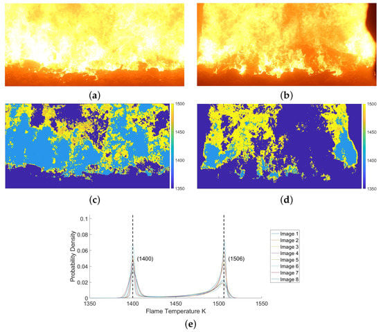
Figure 6.
Furnace images of the same MSW incinerator taken from different angles. (a) Flame image 1; (b) Flame image 2; (c) Flame thermal image 1; (d) Flame thermal image 2; (e) The temperature probability density distribution of the whole flame.
Figure 7 shows the region with temperature between 1398 K and 1402 K is the innermost flame, and the region with temperature between 1504 K and 1508 K is the edge of flame. In summary, the flame temperature distribution has two main modes, which correspond to innermost zone of flame and the edge of flame. The experiments show that the temperature distribution peaks are constant for two modes even if they are captured at different angles and times. Therefore, if the innermost flame and the edge of the flame can be accurately identified, these two characteristics can be used for calibration.

Figure 7.
Two regions of the characteristic temperature in Flame Image 2. (a) Temperature between 1398 K and 1402 K; (b) Temperature between 1504 K and 1508 K.
However, edge area has been changing due to the impact of turbulence. Because of the measuring noise, the non-flame area may also be regarded as the flames. Therefore, it is difficult to accurately determine the location of the edge of the flame. Compared with flame edge, the innermost zone of flame is much easier to be segmented. The innermost flame segmentation algorithm will be described in detail in the next subsection.
4.2. Innermost Flame Segmentation Algorithm
The innermost zone of flame usually has the highest grey value. According to this, Otsu’s method [27] is used to segment the innermost zone easily. It is worth noting that since there are multiple zones of flame, Otsu’s method is required to be performed multiple times to get multilevel threshold. The number of times is adjusted according to the actual division effect, until the area corresponding to the maximum threshold matches the innermost flame. The number usually is 5–8 in practice. At the same time, some morphological operations can be taken to reduce the influence of measurement errors so that few pixels in the non-innermost zone are misclassified into this zone.
The procedure of innermost flame segmentation is as follows:
- 1:
- Transform the original colour image I into the greyscale image ;
- 2:
- The Otsu algorithm [27,28] is used multiple times to calculate the multilevel thresholds for the segmented areas.
- 3:
- Get the binary image using the maximum threshold calculated in step 2;
- 4:
- Morphologically open the binary image in order to reduce misclassification.
4.3. Temperature Distribution Matching Based Calibration Algorithm
Because the area or the number of pixels of the innermost zone in source and reference images are different, one-to-one correspondence between pixels can not be done directly. Based on the discussion in Section 4.1, the temperature distributions in two images are similar. The temperature distributions consist of 2 main modes, whose peaks are almost identical on different images. According to this, the calibration of source camera for pyrometry can be formulated as
where stands for the probability density function. is the temperature in reference image, is the temperature in source image and is the pyrometry model parameter. is a function of . Subscripts and non-in are denoted as innermost zone and non-innermost zone respectively. The objective is to minimize the difference between the two characteristic temperatures measured from the source image and the reference image. Substituting the pyrometry model (Equation (9)) into Equation (19):
However, there is no prior information to know what distribution and follow. In order to compute , one solution is to estimate the probability density function (PDF) directly. In this work, the Kernel Density Estimation (KDE) approach [29] is used to estimate the PDF . The KDE approach is suitable for estimating the PDF for univariate random processes [30]. Because and are univariate, the KDE approach is particularly appropriate to estimate .
Assume is a random variable, its probability density function is denoted by , so the estimation of the probability density function at the point through kernel function is as follows:
where stands for the k-th sample of , M denotes the number of samples, and h is the bandwidth. The selection of bandwidth h controls the smoothness of the resulting probability density curve. There are several ways to determine the bandwidth h. Equation (22) could be used to generate a reasonable estimation of the optimal bandwidth while minimizing the approximation of the mean integrated square error [30,31].
where denotes the standard deviation of .
5. Experiment and Validations
5.1. Offline Preparation—Convert a Digital Camera into a Pyrometer in Laboratory
A pyrometry-calibrated camera should be ready prior to the online calibration tests. The Cannon Mark III is used as the reference temperature camera in this paper. It is critical to prevent underexposure or saturation through setting proper camera parameters while doing two-colour pyrometry on flame images. The camera parameters will also affect the accuracy of temperature measurements as described in Section 3.1. Besides, due to the wide range of temperature distribution, it is necessary to use the revised radio pyrometry model (Equation (13)). Table 1 shows the temperature measurement accuracy of different camera parameters and models results.

Table 1.
Comparison of the Calculated Temperature with the Blackbody Furnace.
It can be seen that the revised model (Quadric) is better than the ordinary one (Linear). Higher ISO would cause larger errors. In general, the smaller aperture time is, the better accuracy can be achieved. However, too small ISO and small aperture time might make that the photoelectric response is not obvious, which is called underexposure and would also reduce accuracy. Thus, the ISO and aperture time should be considered together to prevent underexposure or saturation.
In this paper, the camera is configured to record images at 1/800 s with an ISO of 200 and a maximum aperture of f/2.0. The pyrometry model is shown in Equation (13) with the parameters , .
Table 2 gives a comparison between the setting values of blackbody furnace. The maximum error for the temperature is 1.62%. This result has been approved by the local official instrument-testing organization.
Table 2.
Comparison of the Calculated Temperature with the Blackbody Furnace Using the calibrated pyrometer.
5.2. Online Calibration Experiment—A Real Industrial Experiment of MSWI Flame Temperature Measurement
Experiments were conducted on a real industrial MSW incinerator. This incinerator can process more than 600 tons of MSW per day. As shown in Figure 8, there are two video cameras installed in the MSW incinerator. The frame they take does not overlap, and there are three viewing windows in the same height with the cameras.
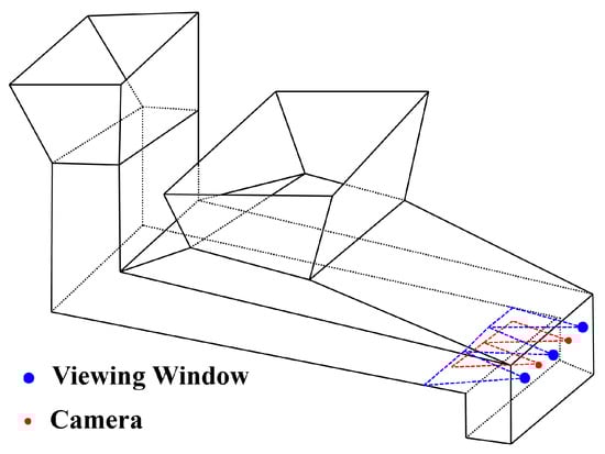
Figure 8.
Schematic of the MSW incinerator’s chamber and the positions of viewing windows and cameras.
The neighbouring camera and the viewing window are close enough to ensure that a common area exists between the reference image captured at the viewing window and the source image captured by the video camera. Thus, this scenario well represents the scene in Figure 3.
The pyrometry-calibrated camera introduced in the last subsection is used as the reference camera, and the left video camera in Figure 8 is used as the source camera. The image taken by the pyrometry-calibrated camera is considered as reference image. The video frame is the source image. Figure 9 shows the source image and the reference image in this case. Although, they are taken at the close position and time, the two images look so different. However, it is easy to see that the grey level of the flame closest to the waste is larger than that of other areas. Thus, the innermost flame segmentation algorithm proposed before still works.
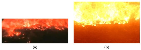
Figure 9.
The reference image and source image of MSWI. (a) Source Image; (b) Reference Image.
The innermost zones of flame in the two pictures are extracted using the algorithm proposed in Section 4.2, as shown in Figure 10. The dark red part of the images is the innermost zone of flame. And the flame temperature in the reference image is estimated using Equation (13) with the parameters chosen in Section 5.1. Next, Equation (21) is employed to estimate the distributions of flame temperature of innermost zone and non-innermost zone. The is 1400.0 K and is 1506.3 K in this case. After computing the ratio of innermost zone and non-innermost zone in source image, interior point method [32] is used to solve Equation (20), and therefore the calibration is completed.

Figure 10.
Innermost zone of Flame Location. (a) Innermost zone of Flame Location of Source Image; (b) Innermost zone of Flame Location of Reference Image.
The temperature distribution of the source image and reference image is shown in Figure 11.

Figure 11.
Result of Temperature Field Measurement. (a) Innermost Source Image; (b) Reference Image.
It can be seen that the flame temperature range in the source image and reference image is close, and it can be considered that the calibration is completed. After the calibration, the temperature distributions measured by video camera maintain two characteristic temperatures. Figure 12 shows the two characteristic temperature variations over time during the image acquisition period. It can be seen that the characteristic temperatures are remained unchanged. This also shows that the previous assumption is true. In summary, due to the temperature distributions and the two characteristic temperatures measured by reference and source camera are similar in the image acquisition period, it could be considered that the online calibration is successful. The temperature measured by this pyrometry-calibrated video camera can be used for the monitoring of combustion status in the waste incinerator. The pyrometry calibrated video camera is in operation since it is deployed in a real MSW incinerator.

Figure 12.
Two characteristic temperatures Blue: lower temperature characteristic Orange: higher temperature characteristic.
6. Conclusions
Flame temperature and its distribution are important for combustion monitoring and control. Although a lot of technologies have been developed to measure the flame temperature distribution, due to the high cost and lack of robustness of instruments, there are still few plants using the advance instruments. On the other hand, the digital camera has been already equipped in almost every plant. For now, it is only used for observing flame morphology and structure. A lot of researches have reported that the digital cameras can be used to measure temperature distribution after being calibrated properly. The traditional calibration methods need to be carried out in the laboratory, so it requires professional laboratory personnel and re-installation of the camera, which is infeasible for practice.
In this paper, a convenient, low-cost, online pyrometer calibration method is proposed. This method takes advantage of the characteristics of the flame temperature distribution and make online calibration possible. The novelty includes:
- 1.
- Only taking one photo by a calibrated pyrometer at a close position to the video camera being used, the calibration can be accomplished.
- 2.
- It significantly reduces the cost and difficulty of pyrometer calibration.
- 3.
- This method can enhance the ability of combustion state diagnosis in a very convenient and cheap way.
Theoretically, the upper limit of the measurement accuracy of this method is the same as the accuracy of the reference pyrometer used. Although the actual measurement accuracy is not strictly verified, in this paper, it is verified that both characteristic temperatures measured with an online calibrated camera over a period of time are close to those measured by a pre-calibrated camera. From this result, the measurement accuracy is sufficient in the combustion monitoring.
Generally speaking, the calibration framework proposed in this paper may also be used on other types of sensors, i.e., calibrating the un-calibrated sensor with the calibrated sensor.
Author Contributions
Conceptualization, C.Z., S.W., Y.C. and S.-H.Y.; methodology, C.Z.; software, C.Z. and S.W.; validation, C.Z., S.W. and B.B.; investigation, B.B.; writing—original draft preparation, C.Z.; writing—review and editing, S.-H.Y. and Y.C.; visualization, C.Z. and S.W.; supervision, S.-H.Y. and Y.C.; funding acquisition, S.-H.Y. All authors have read and agreed to the published version of the manuscript.
Funding
This work was supported by the National Key Research and Development Project of China under Grant No. 2018YFC0214102, and the Institute of Zhejiang University Quzhou Science and Technology Project (IZQ2019-KJ-021).
Data Availability Statement
Not applicable.
Conflicts of Interest
The authors declare no conflict of interest.
References
- Zhang, B.; Xu, C.; Tan, H.; Qi, H.; Sun, J.; Hossain, M.M.; Wang, S. Three-dimensional temperature field measurement of flame using a single light field camera. Opt. Express 2016, 24, 1118–1132. [Google Scholar] [CrossRef]
- Ballester, J.; García-Armingol, T. Diagnostic techniques for the monitoring and control of practical flames. Prog. Energy Combust. Sci. 2010, 36, 375–411. [Google Scholar] [CrossRef]
- Docquier, N.; Candel, S. Combustion control and sensors: A review. Prog. Energy Combust. Sci. 2002, 28, 107–150. [Google Scholar] [CrossRef]
- Sun, J.; Hossain, M.M.; Xu, C.; Zhang, B. Investigation of flame radiation sampling and temperature measurement through light field camera. Int. J. Heat Mass Transf. 2018, 121, 1281–1296. [Google Scholar] [CrossRef]
- Alaruri, S.D.; Brewington, A.J.; Thomas, M.A.; Miller, J.A. High-Temperature Remote Thermometry Using Laser-Induced Fluorescence Decay Lifetime Measurements of Y2O3: Eu and YAG: Tb Thermographic Phosphors. IEEE Trans. Instrum. Meas. 1993, 42, 735–739. [Google Scholar] [CrossRef]
- Gassino, R.; Perrone, G.; Vallan, A. Temperature monitoring with fiber bragg grating sensors in nonuniform conditions. IEEE Trans. Instrum. Meas. 2020, 69, 1336–1343. [Google Scholar] [CrossRef]
- Cao, H.; Yan, X.; Yang, S.; Ren, H.; Ge, S.S. Low-Cost Pyrometry System with Nonlinear Multisense Partial Least Squares. IEEE Trans. Syst. Man Cybern. Syst. 2018, 48, 1029–1038. [Google Scholar] [CrossRef]
- Zhao, W.; Zhang, B.; Xu, C.; Duan, L.; Wang, S. Optical sectioning tomographic reconstruction of three-dimensional flame temperature distribution using single light field camera. IEEE Sens. J. 2018, 18, 528–539. [Google Scholar] [CrossRef]
- Hernández, R.; Ballester, J. Flame imaging as a diagnostic tool for industrial combustion. Combust. Flame 2008, 155, 509–528. [Google Scholar] [CrossRef]
- Gibbins, J.; Lin, Y.M.; Bowden, S.; Cameron, S. Video Observations of Full-Size Pulverised Coal Flames. Combust. Sci. Technol. 2007, 162, 263–280. [Google Scholar] [CrossRef]
- Han, Z.; Hossain, M.M.; Wang, Y.; Li, J.; Xu, C. Combustion stability monitoring through flame imaging and stacked sparse autoencoder based deep neural network. Appl. Energy 2020, 259, 114159. [Google Scholar] [CrossRef]
- Tóth, P.; Garami, A.; Csordás, B. Image-based deep neural network prediction of the heat output of a step-grate biomass boiler. Appl. Energy 2017, 200, 155–169. [Google Scholar] [CrossRef]
- González-Cencerrado, A.; Peña, B.; Gil, A. Coal flame characterization by means of digital image processing in a semi-industrial scale PF swirl burner. Appl. Energy 2012, 94, 375–384. [Google Scholar] [CrossRef]
- Chen, J.; Chan, L.L.T.; Cheng, Y.C. Gaussian process regression based optimal design of combustion systems using flame images. Appl. Energy 2013, 111, 153–160. [Google Scholar] [CrossRef]
- Chen, J.; Chang, Y.H.; Cheng, Y.C.; Hsu, C.K. Design of image-based control loops for industrial combustion processes. Appl. Energy 2012, 94, 13–21. [Google Scholar] [CrossRef]
- Lu, C.; Wang, Z.; Zhou, B. Intelligent fault diagnosis of rolling bearing using hierarchical convolutional network based health state classification. Adv. Eng. Inform. 2017, 32, 139–151. [Google Scholar] [CrossRef]
- Karniadakis, G.E.; Kevrekidis, I.G.; Lu, L.; Perdikaris, P.; Wang, S.; Yang, L. Physics-informed machine learning. Nat. Rev. Phys. 2021, 3, 422–440. [Google Scholar] [CrossRef]
- Raissi, M.; Perdikaris, P.; Karniadakis, G.E. Physics-informed neural networks: A deep learning framework for solving forward and inverse problems involving nonlinear partial differential equations. J. Comput. Phys. 2019, 378, 686–707. [Google Scholar] [CrossRef]
- Aphale, S.S.; DesJardin, P.E. Development of a non-intrusive radiative heat flux measurement for upward flame spread using DSLR camera based two-color pyrometry. Combust. Flame 2019, 210, 262–278. [Google Scholar] [CrossRef]
- Zhao, H.; Feng, H.; Xu, Z.; Li, Q. Research on temperature distribution of combustion flames based on high dynamic range imaging. Opt. & Laser Technol. 2007, 39, 1351–1359. [Google Scholar] [CrossRef]
- Khan, M.A.; Allemand, C.; Eagar, T.W. Noncontact temperature measurement. I. Interpolation based techniques. Rev. Sci. Instrum. 1998, 62, 392. [Google Scholar] [CrossRef]
- Magunov, A. Spectral pyrometry. Instrum. Exp. Tech. 2009, 52, 451–472. [Google Scholar] [CrossRef]
- Yan, W.; Zhou, H.; Jiang, Z.; Lou, C.; Zhang, X.; Chen, D. Experiments on Measurement of Temperature and Emissivity of Municipal Solid Waste (MSW) Combustion by Spectral Analysis and Image Processing in Visible Spectrum. Energy Fuels 2013, 27, 6754–6762. [Google Scholar] [CrossRef]
- Zitová, B.; Flusser, J. Image registration methods: A survey. Image Vis. Comput. 2003, 21, 977–1000. [Google Scholar] [CrossRef]
- Dixon-Lewis G, N. Flame structure and flame reaction kinetics II. Transport phenomena in multicomponent systems. Proc. R. Soc. London. Ser. A Math. Phys. Sci. 1968, 307, 111–135. [Google Scholar] [CrossRef]
- Yu, M.; Lin, J.; Chan, T. Numerical simulation of nanoparticle synthesis in diffusion flame reactor. Powder Technol. 2008, 181, 9–20. [Google Scholar] [CrossRef]
- Otsu, N. Threshold selection method from gray-level histograms. IEEE Trans Syst Man Cybern 1979. [Google Scholar] [CrossRef]
- Aziz, M.A.E.; Ewees, A.A.; Hassanien, A.E. Whale Optimization Algorithm and Moth-Flame Optimization for multilevel thresholding image segmentation. Expert Syst. Appl. 2017, 83, 242–256. [Google Scholar] [CrossRef]
- Hill, P.D. Kernel Estimation of a Distribution Function. Commun. Stat.—Theory Methods 1985, 14, 605–620. [Google Scholar] [CrossRef]
- Kafadar, K.; Bowman, A.W.; Azzalini, A. Applied Smoothing Techniques for Data Analysis: The Kernel Approach with S-PLUS Illustrations. J. Am. Stat. Assoc. 1999, 94, 982. [Google Scholar] [CrossRef] [Green Version]
- Shen, X.; Agrawal, S. Kernel density estimation for an anomaly based intrusion detection system. In Proceedings of the International Conference on Machine Learning; Models, Technologies and Applications, Las Vegas, NV, USA, 26–29 June 2006; pp. 161–167. [Google Scholar]
- Byrd, R.H.; Hribar, M.E.; Nocedal, J. An interior point algorithm for large-scale nonlinear programming. SIAM J. Optim. 1999, 9, 877–900. [Google Scholar] [CrossRef]
Publisher’s Note: MDPI stays neutral with regard to jurisdictional claims in published maps and institutional affiliations. |
© 2022 by the authors. Licensee MDPI, Basel, Switzerland. This article is an open access article distributed under the terms and conditions of the Creative Commons Attribution (CC BY) license (https://creativecommons.org/licenses/by/4.0/).