A Multiobjective Variable Neighborhood Search with Learning and Swarm for Permutation Flowshop Scheduling with Sequence-Dependent Setup Times

Abstract

In recent years, the permutation flowshop scheduling problem (PFSP) with sequence-dependent setup times has been widely investigated in the literature, most focusing on the single-objective optimization problem. However, in a practical production environment, schedulers usually need to handle several conflicting objectives simultaneously, which makes the multiobjective PFSP with sequence-dependent setup times (MOPFSP-SDST) more difficult and time consuming to be solved. Therefore, this paper proposes a learning and swarm based multiobjective variable neighborhood search (LS-MOVNS) for this problem to minimize makespan and total flowtime. The main characteristic of the proposed LS-MOVNS is that it can achieve the balance between exploration and exploitation by integrating swarm-based search with VNS in the multiobjective environment through machine learning technique. For example, the learning-based selection of solutions for multiobjective local search and the adaptive determination of neighborhood sequence to perform the local search are presented based on clustering and statistics to improve the search efficiency. Experimental results on benchmark problems illustrate that the proposed LS-MOVNS algorithm is very effective and competitive to solve MOPFSP-SDST.

1. Introduction

The permutation flowshop scheduling problem (PFSP) is a famous NP-hard combinatorial optimization problem. In this problem, there is a set of n jobs to be processed on a set of m machines. As a flowshop, each job i (i = 1, 2, …, n) must be processed on these m machines in the same order of machine 1, machine 2, …, and machine m. The processing time of each job i on machine j is denoted as p_ij, which is a fixed and nonnegative value. All jobs are available at time zero and once started, the processing of a job cannot be interrupted. It is also assumed that at any time each job can be processed on at most one machine, and each machine can process at most one job. During processing, each job i cannot enter the next machine j for processing until it has been completed on the previous machine j−1 and machine j is available. The task of PFSP is to determine the processing sequence of the n jobs on the m machines so that a certain performance metric can be optimized. There are mainly two performance metrics that are studied most in the literature, i.e., the minimization of makespan (C_max) and the minimization of total flowtime (TFT).

If π = (π₁, π₂, …, π_n) represents a processing permutation of these n jobs, and π_k is the index of the job arranged at the k-th position of the sequence, then the completion time of job π_k on each machine j can be calculated as follows:

$$\begin{array}{l}{C}_{{\pi }_1,1}=p_{{\pi }_1,1}\\ C_{{\pi }_1,j}=C_{{\pi }_1,j-1}+p_{{\pi }_1,j},j=2,3,\dots ,m;\\ C_{{\pi }_k,1}=C_{{\pi }_{k-1},1}+p_{{\pi }_k,1},k=2,3,\dots ,n;\\ C_{{\pi }_k,j}=\max \left\{C_{{\pi }_k,j-1},C_{{\pi }_{k-1},j}\right\}+p_{{\pi }_k,j},k=2,3,\dots ,n;j=2,3,\dots ,m.\end{array}$$

Based on the above calculation, the makespan of the job sequence π can be defined as C_max(π) = $C_{{\pi }_n,m}$, and the total flowtime can be defined as the sum of completion times of all jobs TFT(π) = ${\displaystyle {\sum }_{k=1}^n{C}_{{\pi }_k,m}}$.

Due to its strong industrial background, many variants of PFSP have been studied in the literature [1,2]. Even now, PFSP is still a hot research problem in the field of combinatorial optimization and production scheduling, and many kinds of powerful algorithms have been proposed. For example, Ruiz et al. [3] proposed a powerful iterated greedy method for the distributed PFSP, and Pan et al. [4] developed several effective heuristics and metaheuristics for the distributed PFSP. Later Li et al. [5] further took into account the parallel batching and deteriorating jobs into the distributed PFSP and proposed a hybrid artificial bee colony algorithm. Meng et al. [6] investigated the distributed heterogeneous PFSP with carryover sequence-dependent setup time and designed an enhanced artificial bee colony algorithm to minimize makespan among factories. Pan et al. [7] developed nine metaheuristics for the PFSP with sequence-dependent setup times, among which the first six metaheuristics were trajectory-based algorithms and the other three were population-based algorithms. Recently, Engin and Guclu [8] studied the no-wait flowshop scheduling problem and proposed a new hybrid ant colony optimization algorithm. Huang et al. [9] focused on the distributed assembly permutation flowshop scheduling problem and proposed an improved iterated greedy algorithm. Later, Li et al. [10] investigated the distributed assembly mixed no-idle permutation flowshop scheduling problem, and presented a referenced iterated greedy algorithm to minimize the total tardiness metric. Perez-Gonzalez et al. [11] considered the periodic maintenance in PFSP and proposed several heuristics to minimize makespan. Brammera et al. [12] studied PFSP with multiple lines and demand plans and proposed a reinforcement learning algorithm. Libralesso et al. [13] developed an iterative beam search algorithm for the PFSP to minimize makespan and flowtime. Several powerful metaheuristics were proposed by Silva et al. [14] for the PFSP with a weighted quadratic tardiness objective.

2. Literature Review of MOPFSP and Motivation

As shown in the above section, most of the research on PFSP focused on the single objective optimization. However, in a practical production environment, schedulers often need to optimize two common objectives, e.g., makespan and total flowtime. The two metrics were often taken as the optimization objectives in MOPFSP [15,16,17,18,19,20].

2.1. Literature Review of MOPFSP

Since PFSP usually requires the optimization of multiple conflicting objectives in practical production environments, a great deal of effort has also been devoted to the multiobjective PFSP (MOPFSP) [15,16]. Varadharajan and Rajendran [17] developed a multiobjective simulated-annealing algorithm for the MOPFSP to minimize the makespan and total flowtime of jobs. Pasupathy et al. [18] also dealt with the MOPFSP to minimize the makespan and total flowtime and proposed a multiobjective genetic algorithm. Geiger [19] investigated the topology of search space of MOPFSP with minimization of the makespan and total flowtime. Motair [20] proposed an insertion-based metaheuristic for the MOPFSP to minimize the makespan and total flowtime. A multiobjective memetic algorithm that incorporated local search in genetic algorithm was proposed by Ishibuchi et al. [21] for the MOPFSP. Another version of genetic algorithm hybrid with local search (MOGALS) was developed by Arroyo and Armentano [22]. A mutliobjective particle swarm optimization algorithm was presented by Rahimi-vahed and Mirghorbani [23] for the MOPFSP to minimize flowtime and total tardiness. Promising results were obtained by a multiobjective iterated greedy search proposed by Framinan and Leisten [24]. The state-of-the-art metaheuristics for MOPFSO with two objectives were reviewed and compared by Minella et al. [15], and later a new powerful algorithm named the restarted iterated Pareto greedy (RIPG) algorithm was constructed in Minella et al. [25], which was the best algorithm for bi-objective PFSP in that time. An improved NSGA-II based on a NEH-based local search was proposed by Chiang et al. [26]. Li and Ma [27] proposed a multiobjective memetic algorithm in which an insertion-based local search was embedded for the MOPFSP. A multiobjective ant colony algorithm (MOACA) was developed by Rajendran and Ziegler [28] for MOPFSP to minimize the C_max and TFT, and the results showed that the MOACA belonged to the state-of-the-art algorithms. Wang and Tang [29] proposed a novel machine-learning based multiobjective memetic algorithm (MLMA) for MOPFSP. In this algorithm, the clustering method was adopted to select appropriate solutions to perform a local search, and the local search was then performed in an adaptive way based on statistical learning. Computational results illustrated that the proposed MLMA was very effective for MOPFSP and superior to many state-of-the-art algorithms in the literature based on benchmark problems. Fu et al. [30] developed a decomposition based multiobjective genetic algorithm with adaptive multipopulation strategy for the MOPFSP to minimize the makespan, total flowtime and total tardiness simultaneously.

2.2. Our Motivation

According to the above literature review, it can be found that the multiobjective algorithms proposed for MOPFSP generally incorporated local search into the population-based evolutionary algorithms (EAs) and tried to achieve a balance between exploration and exploitation with some strategy. Since a local search is usually time consuming for MOPFSP, the development of the effective hybrid framework of EA and local search has always been a challenging and hot topic for MOPFSP. In recent studies on multiobjective optimization, machine learning and adaptive search mechanisms have been widely investigated [25,31,32,33,34], and the reported computational results illustrate that they can effectively improve the search performance by focusing most of the search efforts on promising regions or solutions. Inspired by this research and the powerful local search ability of variable neighborhood search (VNS) for PFSPs [35,36,37,38,39], this paper develops a multiobjective variable neighborhood search with learning and swarm (LS-MOVNS) for MOPFSP with sequence-dependent setup times. LS-MOVNS is a hybrid framework of swarm-based search and MOVNS based local search. In addition, the clustering-based solution selection method is adopted to ensure that the search of MOVNS is focused on promising solutions instead of all solutions in the swarm, and the adaptive determination of neighborhood sequence is also proposed to further improve the search efficiency. With the help of the swarm-based search mechanism of EA, the global search ability can be achieved for MOVNS. Therefore, the hybrid of swarm-based search and the learning strategies of solution selection and neighborhood sequence can guarantee that a good balance between exploration and exploitation of MOVNS can be achieved.

3. Proposed LS-MOVNS Algorithm

As a typical combinatorial optimization problem, the MOPFSP with sequence-dependent setup times is well known as NP-hard [40], which means that the exact algorithms cannot solve it in polynomial computation time especially when the problem is large. Therefore, metaheuristics become the common method for solving this problem. In the following sections, we will first briefly describe the overall framework of our LS-MOVNS algorithm and then present each component of it in detail.

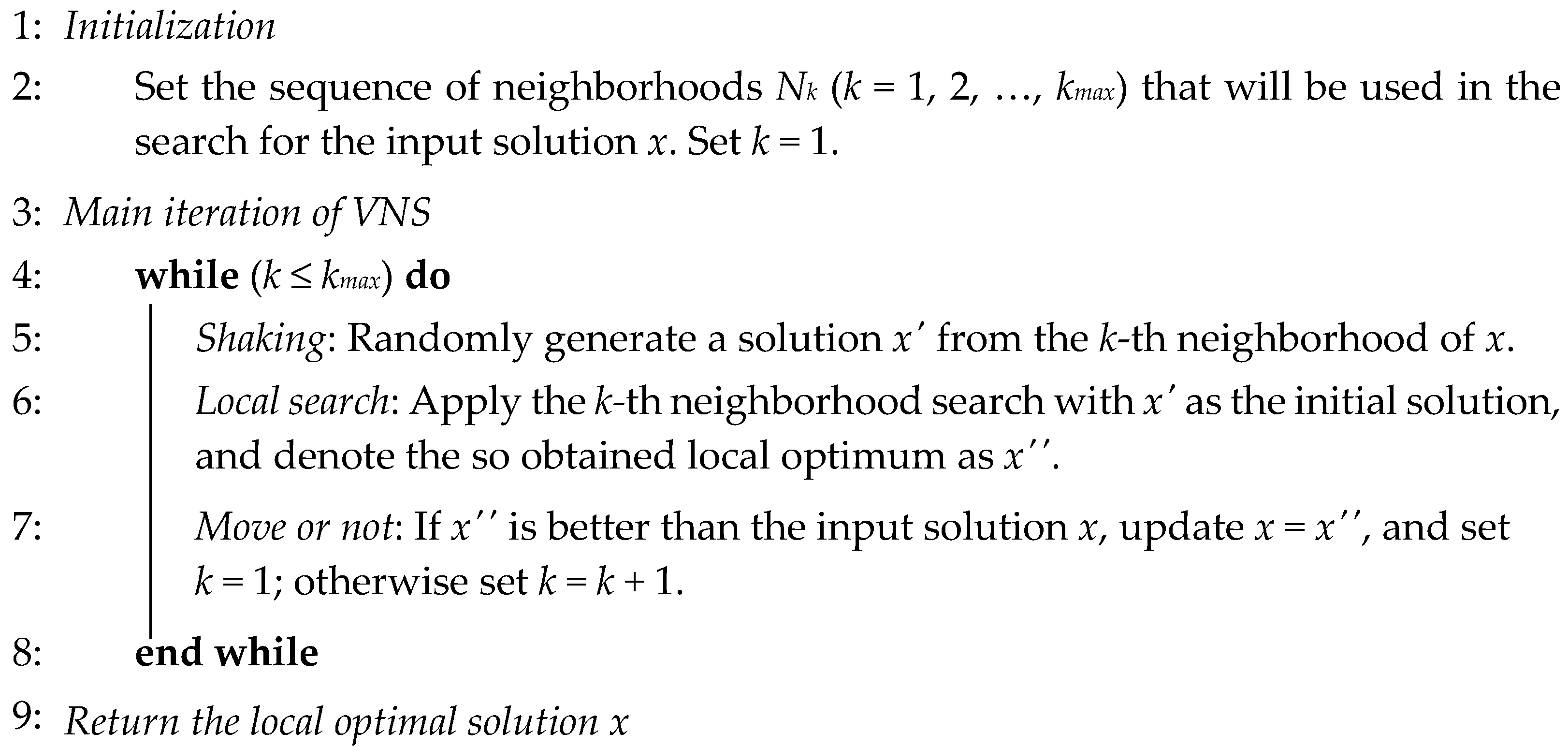
3.1. Traditional VNS

VNS [41] is a simple but effective metaheuristic and its main idea is to use multiple neighborhoods and systematically change the neighborhood within a local search algorithm so as to avoid being trapped in local optimum. The main procedure of traditional VNS, i.e., shaking, local search and move or not, is shown in Algorithm 1.

Algorithm 1: Traditional VNS

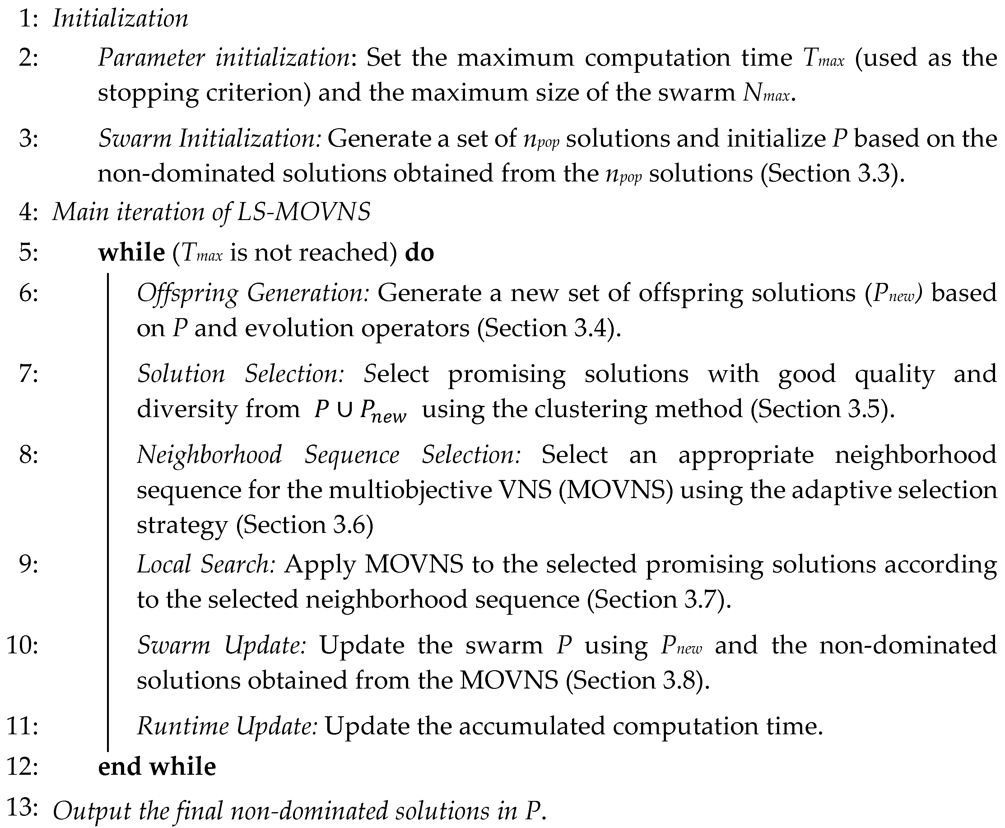
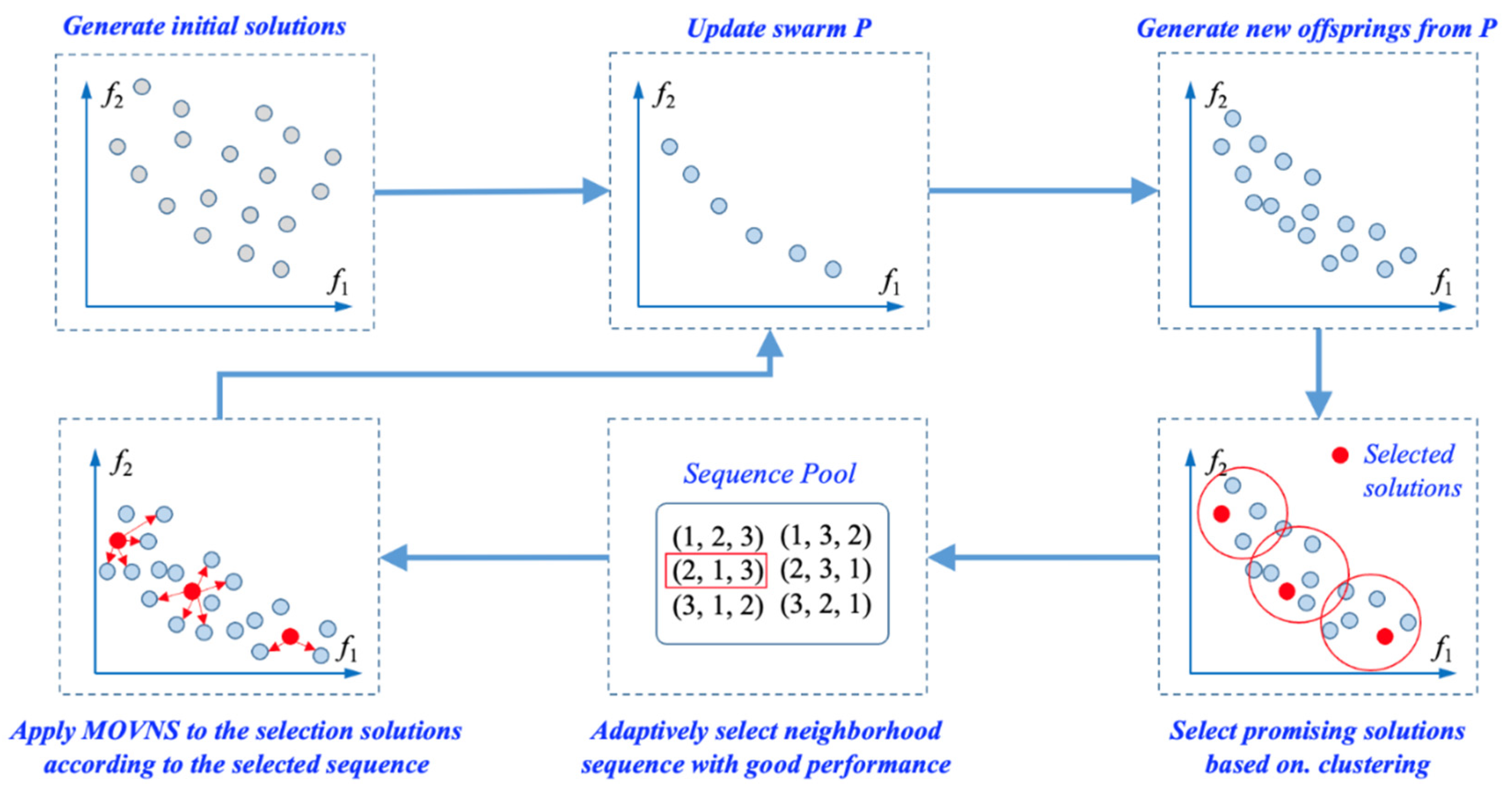
3.2. Overall Framework of the LS-MOVNS

As described in Section 1, the motivation of LS-MOVNS is to take advantage of the good local search ability of VNS and the good global search ability of evolutionary algorithms. Therefore, the overall framework of LS-MOVNS is based on the swarm-based search, and the global search based on genetic operators and the local search based on VNS are alternatively performed during the evolutionary process.

To further improve the search efficiency, specific search strategies are designed for the global search and local search, respectively. For the global search, the swarm search is limited to only the set of non-dominated solutions. That is, the swarm consists of only the non-dominated solutions found during evolution, and the new offspring solutions are generated only from these solutions. For the local search, the clustering method is firstly adopted to determine the promising solutions to perform a local search from the union of the non-dominated solutions and the new offspring. Then, the adaptive strategy is designed to select an appropriate neighborhood sequence to perform the local search. Such a strategy can guarantee that the computational resources are allocated to only the promising solutions with good diversity, instead of the whole population of solutions in traditional evolutionary algorithms, which can save computational resources and thus accelerate convergence. The overall framework and the illustration of the above description are presented in Algorithm 2 and Figure 1, respectively.

Algorithm 2: Overall framework of the LS-MOVNS

3.3. Initialization of the Swarm P

To initialize the swarm P, a set of n solutions are firstly generated in two ways. More specifically, the first two solutions are generated using the NEH heuristic (Nawaz et al. [42]) with the minimization of C_max and TFT, respectively. The procedure of the NEH heuristic can be briefly described as follows.

Step 1.

Calculate the total processing time of each job on all stages, and then sequence all the jobs in non-decreasing order according to the total processing time. Denote the obtained job sequence as Q. Set the partial solution S to be empty.

Step 2.

Insert the first two jobs in Q into the partial solution S so that the increased objective value is minimal, and then delete them from Q.

Step 3.

From the first job in Q, repeat the following procedure, i.e., insert the first job in Q into the partial solution S at the best position that gives the least increased objective function value, and then delete this job from Q, until Q is empty.

Based on the first two solutions in P, the destruction-and-construction method is adopted to generate the other two good quality solutions. The destruction means that we will randomly delete q (q is randomly generated in [2, 5]) adjacent jobs in a given solution x and then each of them will be inserted back to the best position in x according to their deletion sequence. This method will be applied to a solution randomly selected from available initial solutions for n_pop/2 times to generate another n_pop/2 solutions. Finally, the left solutions will be randomly generated.

Based on the n initial solutions, the non-dominated ones from them are selected using the fast non-dominated sorting method in NSGA-II [43] to form the initial swarm P.

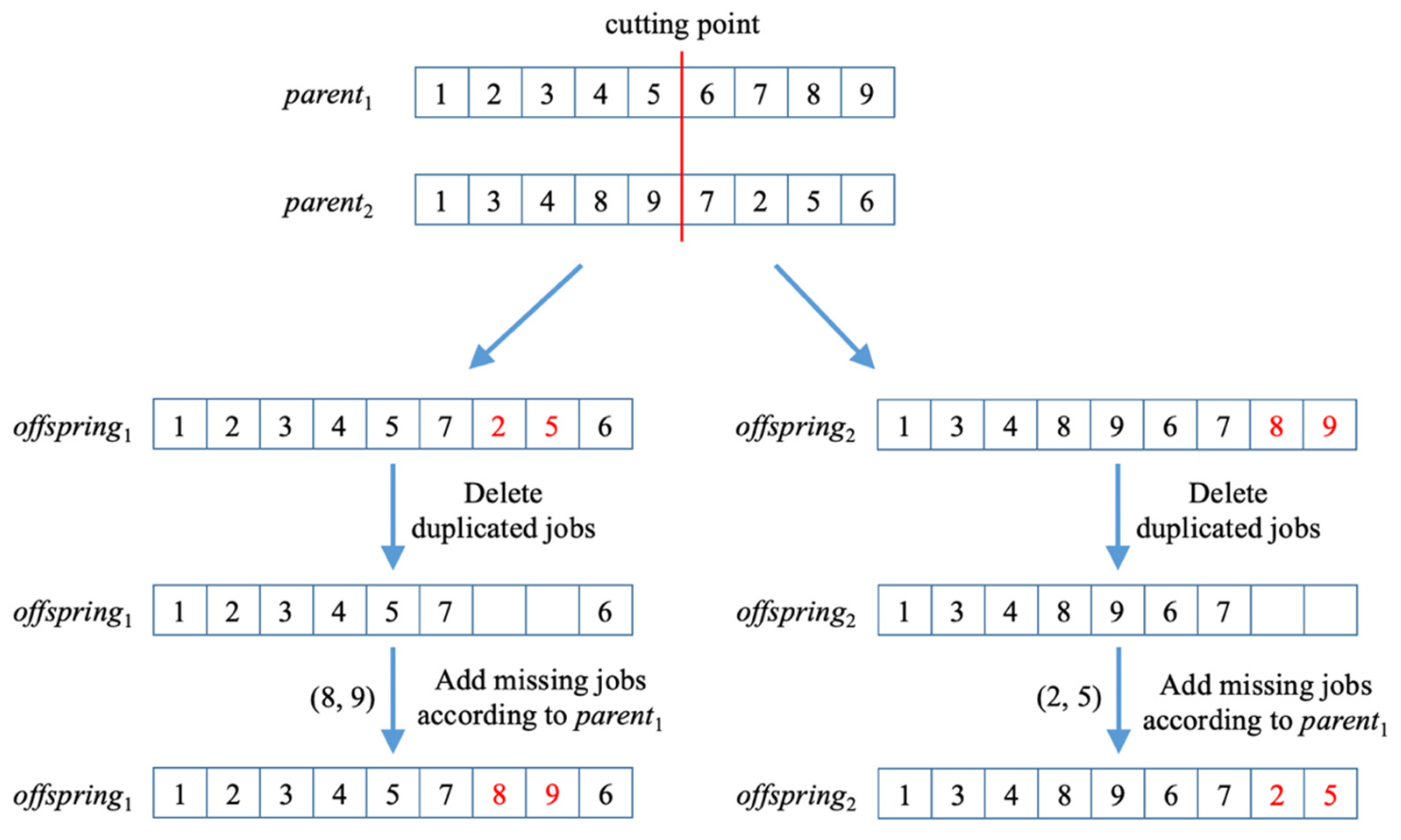
3.4. Generation of New Offspring Solutions

As shown in Algorithm 2 and Figure 1, the generation of new offspring solutions is only based on P, which consists of only the non-dominated solutions found so far.

The generation procedure of new offspring solutions consists of three main steps, as shown in Figure 2. Firstly, two parent solutions will be randomly selected from P. Secondly, the one-point crossover will be used to generate two offspring solutions. Once duplicated solutions are found after crossover, a repair procedure will be adopted to reconstruct the feasibility. The repair procedure will remove the duplicated jobs after the cutting point from the offspring and then add the missing jobs into it according to their original sequence in the first parent. Thirdly, the two offspring solutions will be mutated by randomly swapping two jobs.

3.5. Selection of Promising Solutions with Clustering

It is well known that a local search is time consuming for combinatorial optimization problems, so a clustering-based selection method of promising solutions is adopted to focus the local search only on promising solutions, instead of the whole swarm, so as to save computational resources.

As shown in Figure 1, we first apply the k-Means clustering method to the union of non-dominated solutions in P and the new offspring solutions in P_new. Then for each of the obtained k clusters (the value of k, as well as its impact on the performance of LS-MOVNS, will be discussed in the experiment), we first sequence all the solutions in this cluster in the non-increasing order of their diversity, then randomly select two solutions from the first five solutions in this sequence, and finally the solution with a better Pareto dominance ranking is selected. The diversity of each solution is calculated according to its density, i.e., the distance from it to the l-th (l is set to 5) nearest neighbor solutions in the objective space (please note that the objectives will be normalized during evolution). For a multiobjective problem with minimization objectives, solution x₁ is said to dominate x₂ if and only if $f_i\left(x_1\right)\le f_i\left(x_2\right)$ for each objective i, ($f_i\left(x_1\right)$ denotes the i-th objective of solution x₁) and there exists at least one objective j where $f_j\left(x_1\right)<f_j\left(x_2\right)$. A solution $x^{*}$ is called the Pareto optimal solution if and only if there exists no other solution that can dominate it. The set of all Pareto optimal solutions is called the Pareto set, and correspondingly the set of all the Pareto optimal objective vectors is called the Pareto front. Based on the Pareto dominance, for the two randomly selected solutions x₁ and x₂, x₁ will be selected if it dominates the other solution ns x₂, and vice versa. If they are non-dominated with each other, then the one with better diversity will be selected.

3.6. Adaptive Selection of Neighborhood Sequence for MOVNS

In our LS-MOVNS, there are three kinds of neighborhoods adopted based on the following three neighborhood moves.

• Swap: swap two jobs assigned at two different positions a and b in the solution (i.e., a job sequence).
• Insertion: remove a job from its current position a in the solution and then reinsert it to another position b.
• Two-Swap: perform two different swap moves in the solution.

Since there are three neighborhoods used in the algorithm, there is a total of six different neighborhood sequences that can be adopted in the MOVNS (as shown in Figure 1). In traditional MOVNS, the neighborhood sequence is fixed, such as 1, 2, and 3. That is, the local search is firstly performed in neighborhood 1, neighborhood 2, and neighborhood 3, and once an improved solution is obtained, the search will again go back to neighborhood 1. However, a different sequence may have different performance during evolution, so in our algorithm we propose an adaptive method to select the most appropriate neighborhood sequence for the current search.

The main idea of this adaptive method can be described as follows. Firstly, each sequence has an equal selection probability of 1/6 during the first L generations (i.e., the learning period). At each generation g, the success and failure counts of each selected neighborhood sequence is memorized. Once a certain neighborhood sequence is selected to perform MOVNS on an input solution to generate new solutions, it is considered to be successful if at least one of the new solutions obtained by the local search is not dominated by the input solution (that is, a new solution can dominate the initial solution, or they are both non-dominated with each other). Otherwise, it is considered to have failed. Secondly, when g becomes larger than L, the selection probability of the k-th neighborhood sequence (denoted as p_kg) is calculated according to their success and failure counts during the L generations, that is, $p_{kg}=S_{kg}/{\displaystyle {\sum }_{l=1}^6{S}_{lg}}$ where S_kg denotes the success ratio of the k-th neighborhood sequence in the previous L generations. The success ratio S_kg (k = 1, 2, …, 6) is calculated by $S_{kg}={\displaystyle {\sum }_{l=g-L}^{g-1}{s}_{kl}}/{\displaystyle {\sum }_{l=g-L}^{g-1}(s_{kl}+f_{kl})}+0.01$, g > L, where s_kl and f_kl are, respectively, the success and failure count of the k-th neighborhood sequence. Finally, a neighborhood sequence is adaptively selected for the MOVNS using the roulette wheel method based on the values of p_kg.

3.7. Application of MOVNS

Based on the selected neighborhood sequence, the MOVNS will be applied to each selected promising solution x.

To further accelerate the efficiency of a local search, we do not use the whole neighborhood of a local search in traditional VNS. For example, the neighborhood size of the Insertion neighborhood is n(n − 1), which means that each job is inserted to every other position in the job sequence and thus a total of n(n − 1) new solutions will be generated and evaluated. We make three modifications on such traditional local searches as follows.

First, the insertion action is not executed one by one from the first to the last in the job sequence. Instead, we simply select a job in x at random to perform the insertion action and repeat it n(n − 1)/2 times. Please note that in each case, the chosen job is different from the previously selected ones. With this strategy, only half of the neighborhood is searched and the random selection of different jobs can also guarantee a good diversity of the selected jobs in x.

Second, the local search is a multiobjective search based on Pareto dominance. That is, all the non-dominated solutions obtained from the local search for a solution x will be stored to update the swarm P.

Third, in the stage of “Move or not”, the value of k will be set to be k = k + 1 even if the input solution x is updated by x″. That is, the neighborhood search will not go back to the first one so as to reduce computation resources.

3.8. Update of Swarm P

The update strategy of Pareto front used in NSGA-II is adopted to update the swarm P in our algorithm. For each new solution x, the update procedure can be described as follows.

Step 1.

If solution x is dominated by one solution in P, then solution x is discarded.

Step 2.

If solution x is not dominated by any solution in P, add it to P and then remove all solutions that are dominated by solution x from P.

Step 3.

If the number of solutions in P is larger than a given maximum size N_max, calculate the crowding distance of all solutions in P, and iteratively remove the most crowded solution until |P| = N_max.

4. Experimental Settings

In this section, we first describe the test problems derived from the benchmark problems of MOPFSP in Section 4.1. Then the performance metrics for evaluating the algorithms and the other comparison algorithms are given in Section 4.2. In Section 4.3, the experiment environment and the parameter setting of our LS-MOVNS algorithm is given. Finally, the statistical method used in the experiment to compare the performance of different algorithms is described in Section 4.4.

4.1. Test Problems

In the experiment, the set of 110 benchmark instances for PFSP in Taillard [44] is adopted and we further randomly generate the sequence-dependent setup times for any two jobs on each machine in [0, 50]. These instances are categorized into 11 groups and there are 10 instances with the same problem structure n × m for each group. The number of jobs n and the number of machines m are selected from {20, 50, 100, 200} and {5, 10, 20}, respectively. It should be pointed out that when n = 200, m is selected only from {10, 20}.

4.2. Performance Metrics

Different from the single-objective optimization, the performance of the multiobjecitve algorithm should be evaluated by both the convergence and diversity. Therefore, two important metrics, i.e., the inverted generational distance (IGD) [45] and the hypervolume (HV) [46], are commonly used to evaluate the performance of multiobjective optimization algorithms. Since there is not true Pareto front available for the problem considered in this paper, the reference Pareto optimal front is used to calculate the evaluation metrics. The reference Pareto optimal front for each instance is obtained by the true non-dominated solutions among the union of all the non-dominated solutions obtained by all testing algorithms. The calculation of the two metrics can be briefly described as follows.

Let PF denote the approximate Pareto front obtained by the testing algorithm, $P{F}^{*}$ be the reference Pareto optimal front, and p_j and $p_j^{*}$ be the non-dominated solutions in PF and $P{F}^{*}$, respectively, then the IGD metric can be calculated as

$$IGD\left(PF,P{F}^{*}\right)=\frac{1}{\left|P{F}^{*}\right|}\sqrt{{{\displaystyle \sum }}_{i=1}^{\left|P{F}^{*}\right|}d{\left(p_i^{*},PF\right)}^2},\mathrm{and}d\left(p_i^{*},PF\right)=mi{n}_{j=1}^{\left|PF\right|}\parallel p_i^{*}-p_j\parallel$$

where $d\left(p_i^{*},PF\right)$ is the minimum Euclidean distance from solution $p_i^{*}$ in the reference Pareto front to PF. Please note that a smaller value of IGD means a better performance of the testing algorithm for both convergence and diversity.

The HV metric is calculated as the area covered by the set of non-dominated solutions with comparison to a reference point (please note that the objective values are normalized into [0, 1] in the experiment). The reference point is set to (1.0, 1.0), and, consequently, the maximum value of HV is 1.0. Please note that in the comparison of two Pareto fronts, the higher value of HV means a better performance for both convergence and diversity.

4.3. Experiment Environment and Parameter Setting

All the experiments are carried out on a personal computer with the Intel i7-10700K CPU and 16 GB memory. The parameters of MOVNS-LS are set as follows based on a preliminary test. The size of the solutions to construct the initial swarm P is set to 100 and the maximum size of P is also set to 100. The learning period for the adaptive selection of neighborhood sequence is set as L = 10. The stopping criterion is set to the maximum available CPU time, which is set to n × m × 100 milliseconds. Based on the above description, it can be seen that the proposed algorithm has very few parameters to be adjusted during a search, which makes it simple to be implemented.

4.4. Statistical Method for Performance Comparison

In the experiments, each algorithm was run 10 times independently for each problem instance, so the Wilcoxon rank sum test with a significance level of 0.05 was used to assess whether there was a significant difference between our LS-MOVNS and the comparison algorithms, as conducted in [47]. In the comparison tables in the following sections, the symbols “+”, “−”, and “=” in the Sig column mean that our LS-MOVNS algorithm is significantly better than, worse than, or not significantly different from the comparison algorithm based on the Wilcoxon rank-sum test at a significance level of 0.05 and “Nos. +/−/=” in the last line denotes the count of instances for the above three cases, respectively.

5. Experimental Results

In this section, the sensitivity of the important parameter in our LS-MOVNS was firstly analyzed in Section 5.1 to Section 5.4 which are devoted to illustrating the effectiveness of the improvement strategies proposed in the LS-MOVNS. Finally, the proposed algorithm is compared with some other state-of-the-art algorithms in the literature in Section 5.5.

5.1. Sensitivity Analysis of the Number of Clusters in LS-MOVNS

In the proposed LS-MOVNS, the number of clusters, i.e., the value of k in the k-Means clustering method, determines the number of promising solutions for a local search. That is, it directly determines the computational resources required by the local search, and thus affects the performance of LS-MOVNS. Therefore, in this section the efficiency of this parameter is tested and analyzed. The average IGD metric obtained by different values of k (selected from {2, 4, 6, 8, 10, 12}) for the small-size (20 × 5), medium-size (50 × 5), and large-size groups (100 × 5, 200 × 10) are shown in Figure 3.

As seen in Figure 3, the average IGD metric first decreases as k increases, but then increases significantly when the value of k becomes large for all the three groups of problems. It is clear that the value of k = 6 achieves the best performance. The main reason can be analyzed as follows. First, when the value of k is small (i.e., k = 2), too few solutions are selected for a local search and the search of the algorithm is mainly devoted to the global search, which in turn decreases the search performance. On the contrary, when k is large, most of the computational efforts will be allocated to the local search because more solutions for MOVNS will be too time consuming. Therefore, a medium value of 6 is more appropriate because it can achieve a good balance between a global search and local search. In the following experiments, the value of k is set to 6.

5.2. Effective Analysis of Learning-Based Selection of Solutions for MOVNS

To analyze the effectiveness of the learning-based selection of promising solutions from MOVNS, the LS-MOVNS is compared to its variant in which the promising solution is randomly selected from the swarm P (the variant is denoted as LS-MOVNS_rand). The other parameters are set to the same as those used in the LS-MOVNS.

The comparison results between LS-MOVNS and LS-MOVNS_rand on both the mean and standard deviation (denoted as std) of IGD and HV metrics are shown in

Table 1. Comparison of IGD obtained by LS-MOVNS and LS-MOVNS_rand.

Problem (Jobs × Machines)	LS-MOVNSrand		Sig	LS-MOVNS
	Mean	Std		Mean	Std
20 × 5	1.79 × 10−2	1.4 × 10−2	=	1.76 × 10−2	1.0 × 10−2
20 × 10	2.21 × 10−2	6.7 × 10−3	+	1.93 × 10−2	6.2 × 10−3
20 × 20	5.58 × 10−2	2.8 × 10−2	+	5.36 × 10−2	3.6 × 10−2
50 × 5	2.44 × 10−2	2.4 × 10−2	=	2.39 × 10−2	2.3 × 10−2
50 × 10	3.30 × 10−2	3.9 × 10−2	=	3.25 × 10−2	3.2 × 10−2
50 × 20	3.87 × 10−2	2.1 × 10−2	+	3.64 × 10−2	1.5 × 10−2
100 × 5	2.31 × 10−2	4.1 × 10−2	+	2.00 × 10−2	4.5 × 10−2
100 × 10	4.65 × 10−2	2.1 × 10−2	+	3.92 × 10−2	1.2 × 10−2
100 × 20	2.47 × 10−2	5.6 × 10−3	+	1.99 × 10−2	4.1× 10−3
200 × 10	4.99 × 10−2	5.4 × 10−2	+	4.30 × 10−2	6.4 × 10−2
200 × 20	2.76 × 10−2	4.1 × 10−2	+	1.90 × 10−2	5.3 × 10−2
Nos. +/−/=	8/0/3

and

Table 2. Comparison of HV obtained by LS-MOVNS and LS-MOVNS_rand.

Problem (Jobs × Machines)	LS-MOVNSrand		Sig	LS-MOVNS
	Mean	Std		Mean	Std
20 × 5	5.39 × 10−1	2.1 × 10−1	=	5.36 × 10−1	2.4 × 10−1
20 × 10	4.61 × 10−1	2.2 × 10−1	=	5.07 × 10−1	2.1 × 10−1
20 × 20	3.21 × 10−1	3.4 × 10−1	+	3.43 × 10−1	3.1 × 10−1
50 × 5	4.61 × 10−1	3.8 × 10−1	=	5.65 × 10−1	3.7 × 10−1
50 × 10	4.45 × 10−1	4.1 × 10−1	=	4.42 × 10−1	4.5 × 10−1
50 × 20	3.71 × 10−1	2.5 × 10−1	+	4.05 × 10−1	1.9 × 10−1
100 × 5	5.12 × 10−1	4.3 × 10−1	+	5.91 × 10−1	3.9 × 10−1
100 × 10	4.08 × 10−1	2.2 × 10−1	+	4.24 × 10−1	1.7 × 10−1
100 × 20	4.41 × 10−1	5.4 × 10−1	+	4.95 × 10−1	6.0 × 10−1
200 × 10	5.56 × 10−1	4.9 × 10−1	+	6.07 × 10−1	4.5 × 10−1
200 × 20	5.94 × 10−1	2.6 × 10−1	+	6.57 × 10−1	1.4 × 10−1
Nos. +/−/=	7/0/4

, respectively. In the tables, the symbols “+”, “−”, and “=” mean that our LS-MOVNS algorithm is significantly better than, worse than, or not significantly different from the comparison algorithm based on the Wilcoxon rank-sum test at the significance level of 0.05. and “Nos. +/−/=” in the last line denotes the count of instances for the above three cases, respectively.

From Table 1, it is clear that LS-MOVNS obtains the best results for all the test problems, and among them the performance of our LS-MOVNS algorithm is significantly better than the LS-MOVNS_rand for 8 out of the 11 problem groups. As can be seen in Table 2, LS-MOVNS_rand obtains better results than our LS-MOVNS for only two small size problems (but their performance difference is not significant), while our LS-MOVNS algorithm achieves significantly better results than LS-MOVNS_rand for 7 out of the 11 problem groups. Therefore, it can be concluded that the learning-based selection of promising solutions based on k-Means clustering can help to improve the effectiveness of the local search.

5.3. Effective Analysis of the Adaptive Selection Strategy of Neighborhood Sequence

To verify the adaptive selection strategy of neighborhood sequence, we compared our LS-MOVNS with the variant in which the neighborhood sequence is randomly selected (denoted as LS-MOVNS_{rand_select}).

The comparison results of the IGD metric between the two algorithms are presented in

Table 3. Comparison of IGD obtained by LS-MOVNS and LS-MOVNS_{rand_select}.

Problem (Jobs × Machines)	LS-MOVNSrand_select		Sig	LS-MOVNS
	Mean	Std		Mean	Std
20 × 5	1.75 × 10−2	1.3 × 10−2	=	1.76 × 10−2	1.0 × 10−2
20 × 10	1.91 × 10−2	5.2 × 10−3	=	1.93 × 10−2	6.2 × 10−3
20 × 20	5.31 × 10−2	3.5 × 10−2	=	5.36 × 10−2	3.6 × 10−2
50 × 5	2.42 × 10−2	2.1 × 10−2	=	2.39 × 10−2	2.3 × 10−2
50 × 10	3.37 × 10−2	3.4 × 10−2	+	3.25 × 10−2	3.2 × 10−2
50 × 20	3.81 × 10−2	1.8 × 10−2	+	3.64 × 10−2	1.5 × 10−2
100 × 5	2.18 × 10−2	3.9 × 10−2	+	2.00 × 10−2	4.5 × 10−2
100 × 10	4.35 × 10−2	1.5 × 10−2	+	3.92 × 10−2	1.2 × 10−2
100 × 20	2.27 × 10−2	4.8 × 10−3	+	1.99 × 10−2	4.1× 10−3
200 × 10	4.62 × 10−2	6.1 × 10−2	+	4.30 × 10−2	6.4 × 10−2
200 × 20	2.31 × 10−2	3.7 × 10−2	+	1.90 × 10−2	5.3 × 10−2
Nos. +/−/=	7/0/4

. From this table, it can be seen that LS-MOVNS_{rand_select} can obtain better results for the small size problems. However, as the size of the problem increases, the proposed LS-MOVNS becomes more and more superior, and it can achieve significantly better results than LS-MOVNS_{rand_select} for all the medium- and large-size problems except the group of 50 × 5.

The main reason is that the advantage of the adaptive selection of the neighborhood sequence is not obvious when the number of jobs is small. However, as the number of jobs increases, the size of each neighborhood will increase significantly, and in this situation, the adaptive selection of neighborhood sequenced used in the MOVNS can show great advantage in improving the search efficiency. So, based on the above comparison results and the analysis, it can be concluded that the adaptive selection of the neighborhood sequence is very effective for MOVNS.

5.4. Effective Analysis of the Improved MOVNS

In this experiment, we investigate the effectiveness of the simplified neighborhood search describe in Section 3.6 by comparing our LS-MOVNS (in which only half of the neighborhood size is randomly searched) with its variant in which the neighborhood is fully searched (denoted as LS-MOVNS_full).

The comparison results of IGD metric between the two algorithms are shown in

Table 4. Comparison of IGD obtained by LS-MOVNS and LS-MOVNS_full.

Problem (Jobs × Machines)	LS-MOVNSfull		Sig	LS-MOVNS
	Mean	Std		Mean	Std
20 × 5	1.70 × 10−2	1.3 × 10−2	–	1.76 × 10−2	1.0 × 10−2
20 × 10	1.88 × 10−2	5.2 × 10−3	–	1.93 × 10−2	6.2 × 10−3
20 × 20	5.26 × 10−2	3.5 × 10−2	–	5.36 × 10−2	3.6 × 10−2
50 × 5	2.35 × 10−2	2.1 × 10−2	=	2.39 × 10−2	2.3 × 10−2
50 × 10	3.23 × 10−2	3.4 × 10−2	=	3.25 × 10−2	3.2 × 10−2
50 × 20	3.68 × 10−2	1.8 × 10−2	=	3.64 × 10−2	1.5 × 10−2
100 × 5	2.26 × 10−2	3.9 × 10−2	+	2.00 × 10−2	4.5 × 10−2
100 × 10	4.49 × 10−2	1.5 × 10−2	+	3.92 × 10−2	1.2 × 10−2
100 × 20	2.41 × 10−2	4.8 × 10−3	+	1.99 × 10−2	4.1× 10−3
200 × 10	4.83 × 10−2	6.1 × 10−2	+	4.30 × 10−2	6.4 × 10−2
200 × 20	2.47 × 10−2	3.7 × 10−2	+	1.90 × 10−2	5.3 × 10−2
Nos. +/−/=	5/3/3

. From this table, it can be seen that LS-MOVNS_full obtains better results for the small size and medium size problems, especially for the small size of n = 20 for which its performance is significantly better than that of our algorithm. However, for the large-size problems, the proposed LS-MOVNS becomes more effective, and it can achieve significantly better results than LS-MOVNS_full for all the medium- and large-size problems with n = 100 and n = 200.

The main reason is that the full neighborhood search is more effective than the random search for n = 20 because in such cases the neighborhood size is small and the full search can achieve a better local optimum. However, for large-size problems, the neighborhood size will significantly increase, making the full neighborhood search time consuming. Thus, the evolution generations of the algorithm will decrease within the same available runtime, which limits the global search ability. On the contrary, the random search can save at least half of the computational resources and thus guarantee a better balance of local search and global search, which in turn improves the performance of LS-MOVNS for large-size problems. So, based on the above comparison results and the analysis, it can be concluded that the improved MOVNS is very effective.

5.5. Comparison with Other Powerful Algorithms

In this section, we further compare our LS-MOVNS algorithm with some other powerful algorithms in the literature. The first comparison algorithm is RIPG [25], whose main idea is to iteratively remove a block of jobs in the solution and then re-insert them one by one into the solution. The second comparison algorithm is the MO-MLMA [30], whose main idea is to adopt learning-based methods to determine promising solutions and the application of local search to improve the memetic algorithm. According to the computational results shown in [29], the above two algorithms belong to the state-of-the-art algorithms for MOPFSP in the literature. In the experiment, the two algorithms were implemented in C++ and the source code of MO-MLMA is provided by the original authors. Both of the comparison algorithms share the same stopping criterion and the same maximum size for the non-dominated solutions, as used in our LS-MOVNS.

The comparison results of the IGD and HV metrics obtained by the three algorithms are presented in

Table 5. Comparison of IGD metric obtained by different algorithms.

Problem (Jobs × Machines)	RIPG [26]		Sig	MO-MLMA [30]		Sig	LS-MOVNS
	Mean	Std		Mean	Std		Mean	Std
20 × 5	1.85 × 10−2	1.2 × 10−2	+	1.72 × 10−2	1.4 × 10−2	–	1.76 × 10−2	1.0 × 10−2
20 × 10	2.16 × 10−2	5.1 × 10−3	+	1.98 × 10−2	5.1 × 10−3	=	1.93 × 10−2	6.2 × 10−3
20 × 20	5.67 × 10−2	2.1 × 10−2	+	5.33 × 10−2	3.2 × 10−2	=	5.36 × 10−2	3.6 × 10−2
50 × 5	3.04 × 10−2	2.7 × 10−2	+	2.53 × 10−2	2.1 × 10−2	+	2.39 × 10−2	2.3 × 10−2
50 × 10	3.62 × 10−2	3.3 × 10−2	+	3.24 × 10−2	2.8 × 10−2	=	3.25 × 10−2	3.2 × 10−2
50 × 20	4.07 × 10−2	1.8 × 10−2	+	3.78 × 10−2	2.1 × 10−2	+	3.64 × 10−2	1.5 × 10−2
100 × 5	2.44 × 10−2	4.4 × 10−2	+	2.16 × 10−2	5.1 × 10−2	+	2.00 × 10−2	4.5 × 10−2
100 × 10	4.70 × 10−2	2.5 × 10−2	+	4.12 × 10−2	1.1 × 10−2	+	3.92 × 10−2	1.2 × 10−2
100 × 20	2.53 × 10−2	5.1 × 10−3	+	2.23 × 10−2	3.7 × 10−3	+	1.99 × 10−2	4.1× 10−3
200 × 10	5.42 × 10−2	6.5 × 10−2	+	5.06 × 10−2	5.5 × 10−2	+	4.30 × 10−2	6.4 × 10−2
200 × 20	2.48 × 10−2	5.3 × 10−2	+	2.14 × 10−2	5.7 × 10−2	+	1.90 × 10−2	5.3 × 10−2
Nos. +/−/=	11/0/0			7/1/3

and

Table 6. Comparison of HV metric obtained by different algorithms.

Problem (Jobs × Machines)	RIPG [26]		Sig	MO-MLMA [30]		Sig	LS-MOVNS
	Mean	Std		Mean	Std		Mean	Std
20 × 5	5.25 × 10−1	1.7 × 10−1	+	5.51 × 10−1	1.9 × 10−1	–	5.36 × 10−1	2.4 × 10−1
20 × 10	4.88 × 10−1	2.6 × 10−1	+	5.04 × 10−1	3.4 × 10−1	=	5.07 × 10−1	2.1 × 10−1
20 × 20	3.14 × 10−1	1.6 × 10−1	+	3.47 × 10−1	1.0 × 10−1	–	3.43 × 10−1	3.1 × 10−1
50 × 5	4.85 × 10−1	3.5 × 10−1	+	5.45 × 10−1	2.5 × 10−1	+	5.65 × 10−1	3.7 × 10−1
50 × 10	4.10 × 10−1	4.1 × 10−1	+	4.46 × 10−1	3.8 × 10−1	=	4.42 × 10−1	4.5 × 10−1
50 × 20	3.48 × 10−1	2.6 × 10−1	+	3.97 × 10−1	3.1 × 10−1	=	4.05 × 10−1	1.9 × 10−1
100 × 5	5.46 × 10−1	3.6 × 10−1	+	5.73 × 10−1	4.6 × 10−1	+	5.91 × 10−1	3.9 × 10−1
100 × 10	3.69 × 10−1	2.5 × 10−1	+	4.06 × 10−1	2.2 × 10−1	+	4.24 × 10−1	1.7 × 10−1
100 × 20	4.38 × 10−1	5.0 × 10−1	+	4.78 × 10−1	4.5 × 10−1	+	4.95 × 10−1	6.0 × 10−1
200 × 10	5.36 × 10−1	2.4 × 10−1	+	5.72 × 10−1	3.3 × 10−1	+	6.07 × 10−1	4.5 × 10−1
200 × 20	5.92 × 10−1	2.3 × 10−1	+	6.26 × 10−1	1.2 × 10−1	+	6.57 × 10−1	1.4 × 10−1
Nos. +/−/=	11/0/0			6/2/3

, respectively. In the two tables, the best results are shown in bold style and grey color, while the second-best results are shown in light grey color. From Table 5, it appears that our LS-MOVNS algorithm obtains the best results for 8 of the 11 problem groups, and that the MO-MLMA achieves the best results for 3 out of the 11 problem groups and the second-best results for the left problem groups. In general, our LS-MOVNS outperforms the other two algorithms and the MO-MOLA outperforms the RIPG algorithm. More specifically, LS-MOVNS is significantly better than RIPG for all the test algorithms, and it is significantly better than MO-MLMA for 7 problem groups. Similar observations can be obtained from Table 6 for the HV metric. Therefore, the comparison results illustrate the superiority of our LS-MOVNS for the MOPFSP with sequence-dependent setup times.

The graphical comparisons of our LS-MOVNS and MO-MLMA, i.e., the evolution process of the IGD metric and the obtained Pareto fronts for some problems, are shown in Figure 4 and Figure 5. In Figure 4, the horizon axis is the CPU time (please note that we have divide the maximum available CPU time into 10 parts so that the comparison can be clear for different problem groups), and the vertical axis is the IGD metrics obtained from the current swarm P for our LS-MOVNS algorithm and from the external non-dominated solution set for MO-MLMA [26], respectively. From this figure, it can be observed that our LS-MOVNS has a better convergence speed than MO-MLMA [26]. In Figure 5, we plot the best Pareto front obtained by our LS-MOVNS and MO-MLMA [26] together for four problem groups of 20 × 10, 50 × 10, 100 × 10, and 200 × 10, respectively, in order to clarify the convergence and diversity of the non-dominated solutions in the Pareto front. From this figure, it is clear that our LS-MOVNS has better distribution of Pareto front than MO-MLMA, which further illustrates the efficiency of our algorithm.

6. Further Discussion

In the above experiments, the effectiveness of the proposed LS-MOVNS algorithm has been demonstrated. In this section we further discuss its computational complexity and its potential extension for solving many-objective optimization PFSP problems.

6.1. Computational Complexity

In our algorithm, since the time complexity of computing the objective of a job permutation is O(mn) where m and n are the number of machines and jobs, respectively. The time complexity of NEH that generates the two initial solutions is not more than O(mn³) with a constant coefficient of 2. In the main loop of our LS-MOVNS, the most time-consuming procedures include the k-Means clustering and the MOVNS. Since the k-Means clustering is performed in the bi-objective space, its time complexity is O(t|P|k) with a constant coefficient of 2, in which t = 5 is the iteration of the k-Means clustering, |P| = 100 is the size of the swarm and k = 6 is the number of clusters. For the MOVNS with three neighborhoods, the complexity of the local search for each neighborhood is O(mn³), and there are k = 6 solutions that will be selected for MOVNS. The complexity of the MOVNS is at least O(mn³) with a constant coefficient of 18 (please note that each neighborhood search is applied only once). Since the complexity of k-Means clustering is less than that of MOVNS, so the overall complexity of our LS-MOVNS algorithm is at least O(mn³) with a constant coefficient of 18 × g_max, in which g_max is the corresponding maximum generations of the algorithm within the given available computation time.

6.2. Stopping Criterion of Number of Function Evaluations

Besides the maximum available time, another common adopted stopping criterion is the maximum number of function evaluations. Consequently, we further compared our algorithm with MO-MLMA [20] with 100 mn² function evaluations for n = 20 and 50, and 50 mn² function evaluations for n = 100 and 200, respectively. The comparison results of the IGD metric, as well as the results of Wilcoxon rank-sum test, is shown in

Table 7. Comparison of IGD obtained by MO-MLMA and LS-MOVNS.

Problem (Jobs × Machines)	MO-MLMA [30]		Sig	LS-MOVNS
	Mean	Std		Mean	Std
20 × 5	1.84 × 10−2	1.8 × 10−2	–	1.96 × 10−2	1.4 × 10−2
20 × 10	2.07 × 10−2	4.3 × 10−3	=	1.98 × 10−2	4.7 × 10−3
20 × 20	5.62 × 10−2	2.5 × 10−2	–	5.84 × 10−2	2.1 × 10−2
50 × 5	2.81 × 10−2	3.7 × 10−2	=	2.73 × 10−2	3.4 × 10−2
50 × 10	3.81 × 10−2	3.6 × 10−2	=	3.68 × 10−2	4.1 × 10−2
50 × 20	4.15 × 10−2	2.4 × 10−2	+	3.92 × 10−2	2.6 × 10−2
100 × 5	2.92 × 10−2	3.2 × 10−2	+	2.65 × 10−2	3.7 × 10−2
100 × 10	4.77 × 10−2	2.1 × 10−2	+	4.37 × 10−2	2.5 × 10−2
100 × 20	2.86 × 10−2	3.2 × 10−3	+	2.52 × 10−2	3.7 × 10−3
200 × 10	5.43 × 10−2	4.7 × 10−2	+	4.74 × 10−2	4.3 × 10−2
200 × 20	2.51 × 10−2	3.9 × 10−2	+	2.28 × 10−2	4.4 × 10−2
Nos. +/−/=	6/2/3

. From the comparison results, it can be found that the proposed LS-MOVNS is significantly superior to MO-MLMA [26] for the large-size problems. The MO-MLMA shows advantage over our algorithm only on the small size problems of n = 20 and similar performance on problems with 50 × 5 and 50 × 10. So based on these results, it can be also concluded that our LS-MOVNS outperforms MO-MLMA.

As many researchers have done [15,16,17,18,19,20,21,22,23,24,25,26,27,28,29,30,31], the proposed LS-MOVNS is designed to handle the bi-objective PFSP. However, it has the potential to be extended to many-objective PFSO. For example, the principal component analysis dominance mechanism proposed by Liu et al. [48] could be adopted to handle the solution comparison in the many-objective case. In addition, more challenging objectives such as the time-dependent objective, the environmental, and/or social impact versus productivity objective can be considered. The many-objective optimization and more challenging objectives will be our future studies.

7. Conclusions

In this paper, the MOPFSP with sequence-dependent setup times was investigated, and a multiobjective variable neighborhood search algorithm with learning and swarm was proposed. To better balance the global search and the local search, the swarm evolution was combined with a variable neighborhood search and the clustering was adopted to determine which solution should be selected for the local search. In addition, instead of the traditional fixed neighborhood sequence used in the variable neighborhood search, an adaptive selection strategy was developed based on the performance analysis of different neighborhood sequences. The proposed algorithm was tested on a set of 110 problem instances derived from benchmark set, and the computational results illustrate that the proposed algorithm is very effective and competitive to solve the MOPFSP with sequence-dependent setup times.

References

1. Pan, Q.-K.; Ruiz, R. A comprehensive review and evaluation of permutation flowshop heuristics to minimize flowtime. Comput. Oper. Res. 2013, 40, 117–128. [Google Scholar] [CrossRef]
2. Fernandez-Viagas, V.; Ruiz, R.; Framinan, J.M. A new vision of approximate methods for the permutation flowshop to minimise makespan: State-of-the-art and computational evaluation. Eur. J. Oper. Res. 2017, 257, 707–721. [Google Scholar]
3. Ruiz, R.; Pan, Q.K.; Naderi, B. Terated Greedy methods for the distributed permutation flowshop scheduling problem. OMEGA—Int. J. Manag. Sci. 2019, 83, 213–222. [Google Scholar] [CrossRef]
4. Pan, Q.-K.; Gao, L.; Wang, L.; Liang, J.; Li, X.-Y. Effective heuristics and metaheuristics to minimize total flowtime for the distributed permutation flowshop problem. Expert Syst. Appl. 2019, 124, 309–324. [Google Scholar]
5. Li, J.-Q.; Song, M.-X.; Wang, L.; Duan, P.-Y.; Han, Y.-Y.; Sang, H.-Y.; Pan, Q.-K. Hybrid Artificial Bee Colony Algorithm for a Parallel Batching Distributed Flow-Shop Problem with Deteriorating Jobs. IEEE Trans. Cybern. 2020, 50, 2425–2439. [Google Scholar] [CrossRef] [PubMed]
6. Meng, T.; Pang, Q.K. A distributed heterogeneous permutation flowshop scheduling problem with lot-streaming and carryover sequence-dependent setup time. Swarm Evol. Comput. 2021, 60, 100804. [Google Scholar] [CrossRef]
7. Pan, Q.K.; Gao, L.; Li, X.Y.; Gao, K.Z. Effective metaheuristics for scheduling a hybrid flowshop with sequence-dependent setup times. Appl. Math. Comput. 2017, 303, 89–112. [Google Scholar] [CrossRef]
8. Engin, O.; Guclu, A. A new hybrid ant colony optimization algorithm for solving the no-wait flowshop scheduling problems. Appl. Soft Comput. 2018, 72, 166–176. [Google Scholar] [CrossRef]
9. Huang, Y.-Y.; Pan, Q.-K.; Huang, J.-P.; Suganthan, P.; Gao, L. An improved iterated greedy algorithm for the distributed assembly permutation flowshop scheduling problem. Comput. Ind. Eng. 2021, 152, 107021. [Google Scholar]
10. Li, Y.-Z.; Pan, Q.-K.; Ruiz, R.; Sang, H.-Y. A referenced iterated greedy algorithm for the distributed assembly mixed no-idle permutation flowshop scheduling problem with the total tardiness criterion. Knowl. Based Syst. 2022, 239, 108036. [Google Scholar] [CrossRef]
11. Perez-Gonzalez, P.; Fernandez-Viagas, V.; Framinan, J.M. Permutation flowshop scheduling with periodic maintenance and makespan objective. Comput. Ind. Eng. 2020, 143, 106369. [Google Scholar] [CrossRef]
12. Brammera, J.; Lutzb, B.; Neumann, D. Permutation flow shop scheduling with multiple lines and demand plans using reinforcement learning. Eur. J. Oper. Res. 2022, 299, 75–86. [Google Scholar] [CrossRef]
13. Libralesso, L.; Focke, P.A.; Secardina, A.; Josta, V. Iterative beam search algorithms for the permutation flowshop. Eur. J. Oper. Res. 2022, 301, 217–234. [Google Scholar]
14. Silva, A.F.; Valente, J.M.; Schaller, J.E. Metaheuristics for the permutation flowshop problem with a weighted quadratic tardiness objective. Comput. Oper. Res. 2022, 140, 105691. [Google Scholar]
15. Minella, G.; Ruiz, R.; Ciavotta, M. A Review and Evaluation of Multiobjective Algorithms for the Flowshop Scheduling Problem. INFORMS J. Comput. 2008, 20, 451–471. [Google Scholar] [CrossRef]
16. Sun, Y.; Zhang, C.; Gao, L.; Wang, X. Multi-objective optimization algorithms for flow shop scheduling problem: A review and prospects. Int. J. Adv. Manuf. Technol. 2011, 55, 723–739. [Google Scholar]
17. Varadharajan, T.; Rajendran, C. A multi-objective simulated-annealing algorithm for scheduling in flowshops to minimize the makespan and total flowtime of jobs. Eur. J. Oper. Res. 2005, 167, 772–795. [Google Scholar] [CrossRef]
18. Pasupathy, T.; Rajendran, C.; Suresh, R. A multi-objective genetic algorithm for scheduling in flow shops to minimize the makespan and total flow time of jobs. Int. J. Adv. Manuf. Technol. 2006, 27, 804–815. [Google Scholar] [CrossRef]
19. Geiger, M.J. On operators and search space topology in multi-objective flow shop scheduling. Eur. J. Oper. Res. 2007, 181, 195–206. [Google Scholar] [CrossRef]
20. Motair, H.M. An Insertion Procedure to Solve Hybrid Multiobjective Permutation Flowshop Scheduling Problems. Ind. Eng. Manag. Syst. 2020, 19, 803–811. [Google Scholar] [CrossRef]
21. Ishibuchi, H.; Yoshida, T.; Murata, T. Balance between genetic search and local search in memetic algorithms for multiobjective permutation flowshop scheduling. IEEE Trans. Evol. Comput. 2003, 7, 204–223. [Google Scholar]
22. Arroyo, J.E.C.; Armentano, V.A. Genetic local search for multi-objective flowshop scheduling problems. Eur. J. Oper. Res. 2005, 167, 717–738. [Google Scholar]
23. Rahimi-Vahed, A.R.; Mirghorbani, S.M. A multi-objective particle swarm for a flow shop scheduling problem. J. Comb. Optim. 2007, 13, 79–102. [Google Scholar]
24. Framinan, J.M.; Leisten, R. A multi-objective iterated greedy search for flowshop scheduling with makespan and flowtime criteria. OR Spektrum 2008, 30, 787–804. [Google Scholar]
25. Minella, G.; Ruiz, R.; Ciavotta, M. Restarted Iterated Pareto Greedy algorithm for multi-objective flowshop scheduling problems. Comput. Oper. Res. 2011, 38, 1521–1533. [Google Scholar]
26. Chiang, T.-C.; Cheng, H.-C.; Fu, L.-C. NNMA: An effective memetic algorithm for solving multiobjective permutation flow shop scheduling problems. Expert Syst. Appl. 2011, 38, 5986–5999. [Google Scholar]
27. Li, X.; Ma, S. Multi-Objective Memetic Search Algorithm for Multi-Objective Permutation Flow Shop Scheduling Problem. IEEE Access 2016, 4, 2154–2165. [Google Scholar] [CrossRef]
28. Rajendran, C.; Ziegler, H. A multi-objective ant-colony algorithm for permutation flowshop scheduling to minimize the makespan and total flowtime of jobs. In Computational Intelligence in Flow Shop and Job Shop Scheduling; Chakraborty, U.K., Ed.; Springer: Berlin/Heidelberg, Germany, 2019. [Google Scholar]
29. Wang, X.; Tang, L. A machine-learning based memetic algorithm for the multi-objective permutation flowshop scheduling problem. Comput. Oper. Res. 2017, 79, 60–77. [Google Scholar]
30. Fu, Y.; Wang, H.; Huang, M.; Wang, J. A decomposition based multiobjective genetic algorithm with adaptive multipopulation strategy for flowshop scheduling problem. Nat. Comput. 2019, 18, 757–768. [Google Scholar]
31. Wang, Z.; Zhang, Q.; Li, H.; Ishibuchi, H.; Jiao, L. On the use of two reference points in decomposition based multiobjective evolutionary algorithms. Swarm Evol. Comput. 2017, 34, 89–102. [Google Scholar]
32. Leung, M.-F.; Wang, J. A collaborative neurodynamic approach to multiobjective optimization. IEEE Trans. Neural Networks Learn. Syst. 2018, 29, 5738–5748. [Google Scholar] [CrossRef] [PubMed]
33. Wang, X.; Hu, T.; Tang, L. A multiobjective evolutionary nonlinear ensemble learning with evolutionary feature selection for silicon prediction in blast furnace, IEEE Trans. Neural Netw. Learn. Syst. 2022, 33, 2080–2093. [Google Scholar] [CrossRef] [PubMed]
34. Wang, X.; Dong, Z.; Tang, L.; Zhang, Q. Multiobjective multitask optimization-neighborhood as a bridge for knowledge transfer. IEEE Trans. Evol. Comput. 2022, in press. [Google Scholar] [CrossRef]
35. de Siqueira, E.; Souza, M.; de Souza, S. A Multi-objective Variable Neighborhood Search algorithm for solving the Hybrid Flow Shop Problem. Electron. Notes Discret. Math. 2018, 66, 87–94. [Google Scholar] [CrossRef]
36. Wang, X.; Tang, L. A population-based variable neighborhood search for the single machine total weighted tardiness problem. Comput. Oper. Res. 2009, 36, 2105–2110. [Google Scholar] [CrossRef]
37. Wu, X.; Che, A. Energy-efficient no-wait permutation flow shop scheduling by adaptive multi-objective variable neighborhood search. Omega 2020, 94, 102117. [Google Scholar] [CrossRef]
38. Zhang, X.; Chen, L. A general variable neighborhood search algorithm for a parallel-machine scheduling problem considering machine health conditions and preventive maintenance. Comput. Oper. Res. 2022, 143, 105738. [Google Scholar] [CrossRef]
39. Yazdani, M.; Khalili, S.M.; Babagolzadeh, M.; Jolai, F. A single-machine scheduling problem with multiple unavailability constraints: A mathematical model and an enhanced variable neighborhood search approach. J. Comput. Des. Eng. 2017, 4, 46–59. [Google Scholar] [CrossRef]
40. Garey, M.R.; Johnson, D.S.; Sethi, R. The complexity of flowhsop and jobshop scheduling. Math. Oper. Res. 1976, 1, 117–129. [Google Scholar] [CrossRef]
41. Mladenovic, N.; Hansen, P. Variable neighborhood search. Comput. Oper. Res. 1997, 24, 1097–1100. [Google Scholar] [CrossRef]
42. Nawaz, M.; Enscore, J.E.E.; Ham, I. A heuristic algorithm for the m machine, n job flowshop sequencing problem. Omega 1983, 11, 91–95. [Google Scholar]
43. Deb, K.; Pratap, A.; Agarwal, S.; Meyarivan, T. A fast and elitist multiobjective genetic algorithm: NSGA-II. IEEE Trans. Evol. Comput. 2002, 6, 182–197. [Google Scholar]
44. Taillard, E. Benchmarks for basic scheduling problems. Eur. J. Oper. Res. 1993, 64, 278–285. [Google Scholar]
45. Zitzler, E.; Thiele, L.; Laumanns, M.; Fonseca, C.; da Fonseca, V. Performance assessment of multiobjective optimizers: An analysis and review. IEEE Trans. Evol. Comput. 2003, 7, 117–132. [Google Scholar]
46. Schuetze, O.; Equivel, X.; Lara, A.; Coello Coello, C.A. Some comments on GD and IGD and relations to the Hausdorff distance, In Proceedings of the 12th Annual Conference Companion on Genetic and Evolutionary Computation, ACM. Online, 7 July 2010; pp. 1971–1974. [Google Scholar]
47. Cruz-Rosales, M.H.; Cruz-Chávez, M.A.; Alonso-Pecina, F.; Peralta-Abarca, J.d.C.; Ávila-Melgar, E.Y.; Martínez-Bahena, B.; Enríquez-Urbano, J. Metaheuristic with Cooperative Processes for the University Course Timetabling Problem. Appl. Sci. 2022, 12, 542. [Google Scholar]
48. Liu, Q.; Gui, Z.; Xiong, S.; Zhan, M. A principal component analysis dominance mechanism based many-objective scheduling optimization. Appl. Soft Comput. 2021, 113, 107931. [Google Scholar]
Figure 1. Illustration of the main procedure of the proposed LS-MOVNS.
Processes 10 01786 g001
Figure 2. Illustration of the generation procedure of new offspring solution.
Processes 10 01786 g002
Figure 3. Average of IGD metric obtained by different values of k in LS-MOVNS.
Processes 10 01786 g003
Figure 4. Evolution process of IGD metric obtained by LS–MOVNS and MO–MLMA.
Processes 10 01786 g004
Figure 5. Pareto fronts obtained by LS-MOVNS and MO-MLMA.
Processes 10 01786 g005