Improvement of an Artificial Intelligence Algorithm Prediction Model Based on the Similarity Method: A Case Study of Office Building Cooling Load Prediction

Abstract

Artificial intelligence algorithms (AIAs) have gained widespread adoption in air conditioning load prediction. However, their prediction accuracy is substantially influenced by the quality of training samples. To improve the prediction accuracy of air conditioning load, this study presents an AIA prediction model based on the method of similarity sample screening. Initially, the comprehensive similarity coefficient between samples was obtained by using the gray correlation method improved with information entropy. Subsequently, a subset of closely related samples was extracted from the original dataset and employed to train the artificial intelligence prediction model. Finally, the trained AIA prediction model was used to predict the air conditioning load. The results illustrate that the method of similarity sample screening effectively improved the prediction accuracy of BP neural network (BPNN) and extreme learning machine (ELM) prediction models. However, it is essential to note that this approach may not be suitable for genetic algorithm BPNN (GABPNN) and support vector regression (SVR) models.

1. Introduction

The energy consumption of buildings in China accounts for approximately 30% of the total social energy consumption, while in Europe and OECD countries, this figure exceeds 40% [1,2,3]. This substantial energy usage in buildings significantly contributes to global warming, climate change, and air pollution [4]. The air conditioning system stands out among the energy-consuming components of buildings, responsible for 40–60% of the total energy consumption [5,6]. As a result, reducing energy consumption in air conditioning systems is crucial for sustainable, low-carbon development of buildings.

Air conditioning load prediction plays a pivotal role in energy system planning and the development of efficient air conditioning system operation strategies. Early hour-by-hour air conditioning load prediction models were primarily constructed using the transfer function method, which exhibited low prediction accuracy and limited generalization capability. Consequently, numerous researchers have explored alternative prediction models for air conditioning load forecasting. Wang et al. [7] introduced a combined prediction model, demonstrating its superior accuracy and stability compared to those of previous models. Yun et al. [8] proposed an autoregressive prediction model incorporating exogenous time and temperature indices, achieving prediction accuracy similar to that of the back propagation neural network (BPNN) model and outperforming traditional autoregressive models. Kwok and Lee [9] presented a probabilistic entropy-based neural network prediction model, incorporating six outdoor meteorological parameters and accounting for dynamic building occupancy factors. Their results highlighted the significant impact of building occupancy factors on cooling load prediction and the improved accuracy of the model when considering these factors. Al-Shammari et al. [10] introduced a support vector machine (SVM) prediction model coupled with a firefly optimization algorithm, surpassing genetic planning and artificial neural network models in prediction accuracy. Sajjadi et al. [11] proposed an extreme learning machine (ELM) prediction model, comparing it with genetic planning and BPNN models in regional short-term heat load prediction, with ELM demonstrating superior accuracy. Leung et al. [12] presented a neural network prediction model utilizing the Levenberg–Marquardt algorithm, incorporating seven outdoor meteorological parameters, electricity consumption, and date types of building occupancy space. Their results showed that considering factors such as electricity consumption and building occupancy space type would improve the prediction accuracy significantly. Ilbeigi et al. [13] developed a trained multi-layer perceptron (MLP) model, incorporating artificial neural networks and genetic algorithms to predict building energy consumption accurately. The proposed model exhibited applicability in predicting and optimizing energy consumption for similar buildings. Fan et al. [14] introduced a short-term cooling load prediction model based on deep-learning algorithms, demonstrating substantial improvement in cooling load prediction through unsupervised deep learning for feature extraction. Duanmu et al. [15] recognized the insufficiency of basic building information in urban planning. They introduced a prediction model based on cooling load factors, which yielded a prediction error of less than 20% in general. Yao et al. [16] proposed a combined hour-by-hour cooling load prediction model based on hierarchical analysis, determining weight values for multiple linear regression, autoregressive sliding average, artificial neural network, and gray prediction models through hierarchical analysis. The results indicated that the combined model based on hierarchical analysis achieved higher prediction accuracy than individual models. Ding et al. [17] introduced integrated models combining genetic algorithms with support vector regression (SVR) and wavelet analysis, comparing their effects on short-term and ultra-short-term cooling load predictions. The results showed that the genetic algorithm–SVR model delivered high accuracy for short-term cooling load predictions. In contrast, the genetic algorithm–wavelet analysis–SVR model excelled in ultra-short-term cooling load prediction.

Different prediction models offer their advantages and disadvantages, and in most cases, their prediction accuracy is deemed acceptable. The relatively simple linear regression model often needs to improve in delivering satisfactory prediction outcomes. On the other hand, gray box models offer the benefit of not requiring a deep understanding of their internal mechanisms, making their prediction process relatively straightforward. However, the accuracy of these models tends to diminish when dealing with highly discrete data.

Artificial intelligence algorithms (AIAs) have found wide-ranging applications in air conditioning load prediction, but they still have shortcomings. AIAs frequently demand a significant volume of historical data as training samples to enhance prediction accuracy. However, in practical engineering scenarios, obtaining a sufficient number of effective training samples is often challenging. In addition, samples that lack relevance to the specific prediction moments can introduce interference into the neural network’s training process, potentially leading to local convergence during the iterative process, thereby compromising the model’s predictive accuracy. Hence, focusing on the key factors influencing short-term air conditioning load prediction, this study introduces an AIA prediction model for air conditioning cooling load based on the similarity sample screening method. The primary objective is to enhance the prediction accuracy of commonly used AIAs.

A correlation analysis method was employed to identify the primary factors impacting air conditioning load changes first. This analysis process aided in reducing the dimensionality of input samples and simplifying the prediction model. Subsequently, the gray correlation method improved with the information entropy method was utilized to assess the degree of similarity between samples. The original samples were then pre-processed based on their similarity, eliminating training samples that bore little relevance to the input variables at the prediction moment and mitigating the interference of anomalous samples during the training and learning processes of AIAs. Finally, this refined set of training samples was integrated into the standard AIA prediction model, thereby elevating the model’s predictive accuracy.

The rest of this paper is organized as follows: Section 2 describes the conventional AIA prediction model and the improved prediction processes in detail. Section 3 introduces the case building located in Tianjin to evaluate the performance of the improved method. Finally, Section 4 provides conclusions and possible future works.

2. Methodologies

2.1. Air Conditioning Load Prediction Model Based on Conventional AIA

2.1.1. BPNN Prediction Model

A BPNN is a multi-layer feed-forward neural network that relies on error back propagation. It is widely recognized as a quintessential supervised learning algorithm. This neural network model employs non-linear transfer functions, enabling neurons in each hidden layer to acquire the capacity to learn. Throughout its training process, the network utilizes the gradient descent learning rule, which facilitates the minimization of global error, ultimately aiming to attain the optimal expected value. In instances where the training error fails to meet the predefined accuracy criteria, the weights and thresholds of each neuron are iteratively adjusted through back propagation, starting from the output layer and progressing towards the input layer until the output error aligns with the specified accuracy threshold.

The structure of a typical three-layer (single hidden layer) BPNN is shown in Figure 1.

As illustrated in Figure 1, a typical three-layer BPNN typically comprises an input layer, a hidden layer, and an output layer, with interconnected neurons extending from one layer to the next (from the input layer to the hidden layer and from the hidden layer to the output layer). Neurons within the same layer, however, are not interconnected.

The quantity of neurons in the hidden layer, situated between the input and output layers, is typically determined based on the structural characteristics of the input samples. The formula for calculating the number of neurons in the hidden layer is expressed in Equation (1) [18,19]:

$$l=2\times p+1$$

(1)

where l is the number of neurons in the hidden layer, and p is number of neurons in the input layer.

The learning process of a BPNN is shown in Figure 2.

As illustrated in Figure 2, the learning process of a BPNN typically involves the following stages [18,19,20,21]:

In the first step, the initial connection weights and thresholds for the BPNN are randomly assigned within the range of [−0.5, 0.5] as a part of the network’s initialization process.

In the second step, the output values of the neurons in the hidden layer are calculated using specific computational expressions, as detailed in Equations (2) and (3):

$$S_j={\displaystyle \sum _{t=1}^p{\omega }_{jt}{x}_t}-{\alpha }_j$$

(2)

$$H_j=F(S_j)$$

(3)

Here, S_j is the input signal of the hidden layer neuron, H_j is output value of the hidden layer neuron, x_t is the input variable, ω_jt is the connection weights of neurons between the input layer and the hidden layer, α_j is the threshold value of the neuron in the hidden layer, and F(S) is the transfer function of the hidden layer neuron.

In the third step, the output values of the neurons in the output layer are computed using the computational expressions detailed in Equations (4) and (5):

$$S_k={\displaystyle \sum _{k=1}^o{\psi }_{kj}{H}_j}-{\beta }_k$$

(4)

$$O_k=G(S_k)$$

(5)

where S_k is the input signal of the output layer neuron, O_k is the output value of the output layer neuron, ψ_kj are the connection weights of the neurons between the hidden layer and the output layer, β_k is the threshold value of the output layer neuron, and G(S) is the transfer function of the output layer neuron.

In the fourth step, the error between the output value of a single training sample network and the desired output value is computed as indicated in Equation (6):

$$e_k=\frac{1}{2}{\displaystyle \sum _{k=1}^o{(O_k-E_k)}^2}$$

(6)

where e_k is the computational error of a single training sample, and E_k is the desired output value of the BPNN.

In the fifth step, the connection weights and thresholds of the neurons in the hidden and output layers are updated, as demonstrated in Equations (7)–(10):

$${\omega }_{jt}^{N+1}={\omega }_{jt}^N+\mu ({\omega }_{jt}^N-{\omega }_{jt}^{N-1})+(1-\mu )\eta {\delta }_j{x}_t$$

(7)

$${\psi }_{kj}^{N+1}={\psi }_{kj}^N+\mu ({\psi }_{kj}^N-{\psi }_{kj}^{N-1})+(1-\mu )\eta {\delta }_k{H}_j$$

(8)

$${\alpha }_j^{N+1}={\alpha }_j^N+\eta {\delta }_j$$

(9)

$${\beta }_k^{N+1}={\beta }_k^N+\eta {\delta }_k$$

(10)

where η is the learning efficiency of the neural network, δ_j is the partial derivative of the computational error function for the connection weights between neurons in the input and hidden layers, δ_k is the partial derivative of the computational error for the connection weights between the neurons of the hidden and output layers, and μ is the additional momentum coefficient.

In the sixth step, global error is computed as indicated in Equation (11):

$$e_{\mathrm{all}}=\frac{1}{2m}{\displaystyle \sum _{i=1}^m{\displaystyle \sum _{k=1}^o{(O_k-E_k)}^2}}$$

(11)

where e_all is the global error of the BPNN, and m is the total number of training samples.

In the seventh step, it is determined whether the global error of the BPNN meets the set requirements. If the error requirements are satisfied, the iteration ends, and the prediction results are output. If the error requirements are not met, the process returns to the second step for the next round of learning.

2.1.2. Genetic Algorithm BPNN Prediction Model

A BPNN employs the gradient descent learning rule to minimize global error, but it still exhibits issues, including limited model robustness, slow learning and convergence rates, and susceptibility to local minima during the learning process. Moreover, the choice of initial connection weights and thresholds significantly influences the training of a BPNN. The utilization of genetic algorithms for optimizing the learning process of a BPNN can mitigate these concerns to a considerable extent [18]. Thus, the genetic algorithm BPNN (GABPNN) prediction model is generally used to replace the BPNN model for prediction.

The genetic algorithm is a global optimization search technique inspired by Darwin’s principle of “survival of the fittest” in the biological world. Genetic algorithms offer a unique approach, unlike methods that rely on function derivatives and continuity. They encode relevant parameters into a set of chromosomes and employ probabilistic methods for a sequence of iterative operations, including chromosome selection, crossover, and mutation. This process culminates in retaining individuals with high fitness and eliminating those with low fitness. Through this procedure, the offspring inherit information from their parent individuals and adapt more effectively to their environment. This results in the optimization of the entire population [18,22,23,24].

The learning process of a GABPNN is depicted in Figure 3.

As depicted in Figure 3, the learning process of a GABPNN primarily comprises the following three phases: Firstly, the network’s topology is determined, and the initial population for the genetic algorithm is generated. Subsequently, the genetic algorithm is employed to optimize the initial connection weights and thresholds of the BPNN. In the final step, the optimal weights and thresholds obtained in the preceding phase are assigned to the BPNN for training and learning. The concrete steps of the genetic algorithm are shown below [13,18,19,22,23,24]:

The first step is population initialization. Population initialization entails the derivation of the initial solutions for the population in accordance with predefined encoding protocols.

The second step is the calculation of the fitness function. An individual’s fitness within a population serves as the metric by which its quality is assessed. A better fitness value corresponds to heightened adaptability and overall superiority. The formulation of an individual’s fitness function is conventionally expressed in the manner delineated by Equation (12):

$$F=\frac{1}{e_{\mathrm{all}}}$$

(12)

where F is the individual fitness value.

The third step is the selection operation. This operation aims to emulate the natural course of evolution by singling out the most adept individuals from the population while eliminating those with diminished fitness. The calculation of the probability of an individual being selected is explicated in Equation (13):

$$P_l=\frac{F_l}{{\displaystyle \sum _{l=1}^n{F}_l}}$$

(13)

where P_l is the probability of individual l being selected, F_l is the fitness value of the individual, and n is the number of individuals.

Equation (13) elucidates that an individual boasting a heightened fitness value enjoys an augmented likelihood of selection within the population.

The fourth step is the crossover operation. This operation involves the stochastic selection of two parental individuals from the population and the subsequent recombination of select chromosomes to generate a novel individual. The process of the crossover operation is expounded in Equations (14) and (15):

$$a_{qt}=a_{qt}\times (1-b)+a_{st}\times b$$

(14)

$$a_{st}=a_{st}\times (1-b)+a_{qt}\times b$$

(15)

where a_qt, a_st is the new chromosome of the qth chromosome a_q and the sth chromosome a_s recombined by crossover at the t position and b is the random number with values in the range of [0, 1].

The fifth step is the mutation operation. The data representation of the mutation process about the tth gene of the qth individual, X_qt, is elucidated in Equations (16) and (17):

$$f(d)=c\times {(1-\frac{d}{D})}^2$$

(16)

$${X^{\prime }}_{qt}=\left\{\begin{array}{l}{X}_{qt}+(X_{qt}-X_{\max })\cdot f\left(d\right)(r\ge 0.5)\\ X_{qt}+(X_{\min }-X_{qt})\cdot f\left(d\right)(r<0.5)\end{array}\right.$$

(17)

where c is a random number taking values in the range of [0, 1], d is the current iteration number, D is the maximum number of evolution, X′_qt is a mutated gene, X_max is the upper bound of gene X_qt, X_min is the lower bound of gene X_qt, and r is a random number with values in the range of [0, 1].

The sixth step is to determine whether the evolution is terminated or not. Termination is effected when the training error (fitness) of the network satisfies pre-established prerequisites or when the maximum number of iterations is reached. At this juncture, the iterative decoding process concludes, yielding the optimal weights and thresholds, thereby marking the culmination of the evolutionary process. In the event that these termination conditions remain unmet, the process reverts to the third stage, subsequently iterating the computational process until the stipulated termination criteria are met.

2.1.3. SVR Prediction Model

The SVM, introduced by American scholars Cortes and Vapnik in 1995 [25], is a learning algorithm devised to address the challenge of classifying two datasets. This approach entails transforming the non-linear classification problem associated with sample data into a linear classification problem, achieving this through mapping the sample data into a high-dimensional space. Subsequently, Vapnik introduced the ε linear insensitive loss function, paving the way for the development of a real-valued SVM, commonly known as an SVR learning machine [26].

The structure of an SVR learning machine is shown in Figure 4.

As depicted in Figure 4, the input and output layers of an SVR learning machine are interconnected through kernel function nodes. Each kernel function node corresponds to a support vector, and the linear combination of these kernel function nodes forms the output of an SVR learning machine.

Assuming a total of m training samples, the input and output sample sets of the training samples are $\left\{(x_i,y_i)\right\}$ (x_i is the input column vector of the sample $x_i={[x_{i1},x_{i2},\cdots ,x_{ip}]}^{\mathrm{T}}\in R^p$; y_i is the output value of the sample, $y_i\in R$; $i=1,2,\cdots ,m$). The linear relationship between the input and output values of training samples in high-dimensional space is described in Equation (18) [26]:

$$g(x)=V\cdot \phi (x)+v$$

(18)

where g(x) is the output value (the predicted value) of the SVR model, φ(x) is the nonlinear mapping function, V is the weight vector, and v is the linear regression coefficient (intercept).

The specific expression of the ε linear insensitive loss function is shown in Equation (19):

$$L_{\epsilon }(g(x),y)=\left\{\begin{array}{l}0,\left|y-g(x)\right|\le \epsilon \\ \left|y-g(x)-\epsilon \right|,\left|y-g(x)\right|>\epsilon \end{array}\right.$$

(19)

where L_ε(g(x), y) is the ε linear insensitive loss function, and ε is the error requirement for the linear regression function.

The weight vector V and the regression coefficients v are calculated using the regularized risk function as shown in Equation (20):

$$\left\{\begin{array}{l}\underset{{\xi }_i,{\xi }_i^{*},V,v}{\mathrm{Minimize}}:\frac{1}{2}{‖V‖}^2+C{\displaystyle \sum _{i=1}^m({\xi }_i+{\xi }_i^{*})}\\ \mathrm{s}.\mathrm{t}.\left\{\begin{array}{l}{y}_i-V\cdot \phi (x_i)-v\le \epsilon +{\xi }_i^{*}\\ -y_i+V\cdot \phi (x_i)+v\le \epsilon +{\xi }_i\\ {\xi }_i^{*}\ge 0\\ {\xi }_i\ge 0\end{array}\right.\end{array}\right.$$

(20)

where C is the penalty factor, which indicates the degree of punishment for training errors larger than ε. The larger the C indicator, the stronger the punishment, and ξ_i and ξ_i^* are the slack variables.

By introducing the Lagrangian function and performing a pairwise transformation, the solution to Equation (20) can be converted to the solution to Equation (21):

$$\left\{\begin{array}{l}\underset{\alpha ,{\alpha }^{*}}{\mathrm{Maximize}}:-\epsilon {\displaystyle \sum _{i=1}^m({\alpha }_i^{*}+{\alpha }_i)}+{\displaystyle \sum _{i=1}^m{y}_i\cdot ({\alpha }_i^{*}-{\alpha }_i)}-\\ \frac{1}{2}{\displaystyle \sum _{i,r=1}^m({\alpha }_i^{*}-{\alpha }_i)\cdot ({\alpha }_r^{*}-{\alpha }_r)}\cdot K(x_i,x_r)\\ \mathrm{s}.\mathrm{t}.\left\{\begin{array}{l}{\displaystyle \sum _{i=1}^m{\alpha }_i^{*}}={\displaystyle \sum _{i=1}^m{\alpha }_i}\\ 0\le {\alpha }_i^{*}\le C\\ 0\le {\alpha }_i\le C\end{array}\right.\end{array}\right.$$

(21)

where ${\alpha }_i$ and ${\alpha }_i^{*}$ are the Lagrange multipliers, and $K(x_i,x_r)$ is the kernel function, $K(x_i,x_r)=\phi (x_i)\cdot \phi (x_r)$.

The results of solving Equation (21) can be brought into Equation (18) to find the SVR function as shown in Equation (22):

$$g(x)={\displaystyle \sum _{i=1}^m({\alpha }_i^{*}-{\alpha }_i)}\cdot K(x_i,x)+b$$

(22)

2.1.4. ELM Prediction Model

Huang et al. [27] introduced a novel single-hidden-layer feedforward neural network called the ELM in 2004. This innovative algorithm obviates the need to adjust connection weights and thresholds within a neural network according to the gradient descent learning rule during training and learning. Instead, it merely necessitates specifying the number of neurons in the hidden layer and selecting an infinitely differentiable hidden layer transfer function. Subsequently, Huang et al. [28] conducted a comprehensive investigation into the principles and application of the ELM. Their findings demonstrated that the ELM had superior generalization capabilities and a faster learning rate.

The structural diagram of the ELM is similar to that of a typical three-layer BPNN (shown in Figure 1). The input and output sample sets of the training samples are assumed as $\left\{(x_i,y_i)\right\}$ (x_i is the input column vector of the sample. $x_i={[x_{i1},x_{i2},\cdots ,x_{ip}]}^{\mathrm{T}}\in$$R^p$; y_i is the output vector of the sample. ${\mathit{y}}_{\mathit{i}}={[y_{i1},y_{i2},\dots ,y_{io}]}^{\mathrm{T}}\in R^o$; $i=1,2,\cdots ,m$). The expression for the calculation of the output value of the output layer of the neural network is expressed as Equation (23):

$$O_i={\displaystyle \sum _{j=1}^l{\psi }_j}F({\omega }_j\cdot x_i+a_j)$$

(23)

where O_i is the vector of the output values of the neural network output layer, $O_i={[O_{i1},O_{i2},\dots ,O_{io}]}^{\mathrm{T}}$, ω_j is the weight vector between the jth hidden layer and the neurons of the input layer, ${\omega }_j=[{\omega }_{j1},{\omega }_{j2},\dots ,{\omega }_{jp}]$, and ψ_j is the weight vector between the jth hidden layer and the output layer neuron, ${\psi }_j={[{\psi }_{j1},{\psi }_{j2},\dots ,{\psi }_{jo}]}^{\mathrm{T}}$.

Assuming the existence of α_j, ω_j, and ψ_j that make ${\displaystyle \sum _{i=1}^m‖O_i-y_i‖}$ infinitely close to zero, then Equation (23) can be converted to Equation (24):

$$y_i={\displaystyle \sum _{j=1}^l{\psi }_j}F({\omega }_j\cdot x_i+{\alpha }_j)$$

(24)

The matrix expression for m training samples is shown in Equation (25):

$$ZB=T$$

(25)

Here, B is the weight matrix between the neurons of the hidden and output layers of all training samples, Z is the output value matrix of the neurons of the hidden layer of all training samples, and T is the output value matrix of the neurons of the output layer of all training samples.

Mathematical expressions for matrices B, Z, and T are shown in Equations (26), (27), and (28), respectively:

$$B={\left[\begin{array}{c}{\psi }_1^{\mathrm{T}}\\ {\psi }_2^{\mathrm{T}}\\ ⋮\\ {\psi }_l^{\mathrm{T}}\end{array}\right]}_{l\times o}$$

(26)

$${\begin{array}{c}Z({\omega }_1,{\omega }_2,\cdots ,{\omega }_l,{\alpha }_1,{\alpha }_2,\cdots ,{\alpha }_l,x_1,x_2,\cdots ,x_m)=\hfill \\ \left[\begin{array}{cccc}F({\omega }_1\cdot x_1+{\alpha }_1)& F({\omega }_2\cdot x_1+{\alpha }_2)& \cdots & F({\omega }_l\cdot x_1+{\alpha }_l)\\ F({\omega }_1\cdot x_2+{\alpha }_1)& F({\omega }_2\cdot x_2+{\alpha }_2)& \cdots & F({\omega }_l\cdot x_2+{\alpha }_l)\\ ⋮& ⋮& \cdots & ⋮\\ F({\omega }_1\cdot x_m+{\alpha }_1)& F({\omega }_2\cdot x_m+{\alpha }_2)& \cdots & F({\omega }_l\cdot x_m+{\alpha }_l)\end{array}\right]\hfill \end{array}}_{m\times l}$$

(27)

$$T={\left[\begin{array}{c}{y}_1^{\mathrm{T}}\\ y_2^{\mathrm{T}}\\ ⋮\\ y_m^{\mathrm{T}}\end{array}\right]}_{m\times o}$$

(28)

In the training and learning processes of the ELM, wherein values of α_j and ω_j are randomly assigned while maintaining the magnitude of these two parameters constant, the weight matrix B connecting the hidden and output layers can be derived by utilizing the least squares method, as shown in Equation (29):

$$\underset{B}{\min }‖ZB-T‖$$

(29)

By solving Equation (29), the solution of the weight matrix $\widehat{B}$:

$$\widehat{B}=Z^{+}T$$

(30)

Here, Z⁺ is the Moore–Penrose generalized inverse of the hidden layer output matrix Z of the ELM.

2.2. Improved Air Conditioning Load Prediction Model Based on Similarity

2.2.1. Calculation of Comprehensive Similarity Coefficient

This study introduces the concept of a comprehensive similarity coefficient to quantify the similarity between predicted and historical moments of model input variables. Unlike the traditional correlation coefficient, the comprehensive similarity coefficient considers the unique contributions of individual input variables to the overall similarity of the samples. This approach provides a more objective and comprehensive assessment of sample similarity. The calculation of this comprehensive similarity coefficient is based on a combination of the gray correlation method and information entropy, enhancing the rigor and comprehensiveness of the similarity assessment. The detailed computational procedure for determining the comprehensive similarity coefficient is delineated in Figure 5.

• Gray correlation method

The main steps to calculate the comprehensive similarity coefficient using the gray correlation method are as follows:

In the first step, the feature vectors of the input samples of the building cooling load prediction moments and historical moments are first determined, as shown in Equation (31):

$${\mathit{x}}_h=\left[x_{h,1},x_{h,2},\cdots ,x_{h,t},\cdots ,x_{h,p}\right]$$

(31)

where x_h is the input sample feature vector, x_h,p is the input variable eigenvalue, t is the number of input variables, and h is the hth moment, h = 0, 1, 2, …, n, when h = 0, it means the prediction moment, when h ≠ 0, it means the historical moment.

The feature vectors of the input samples from the predicted and historical moments are utilized to form the feature matrix A as shown in Equation (32):

$$\mathit{A}=\left[\begin{array}{cccccc}{x}_{0,1}& x_{0,2}& \cdots & x_{0,t}& \cdots & x_{0,p}\\ x_{1,1}& x_{1,2}& \cdots & x_{1,t}& \cdots & x_{1,p}\\ ⋮& ⋮& ⋮& ⋮& ⋮& ⋮\\ x_{h,1}& x_{h,2}& \cdots & x_{h,t}& \cdots & x_{h,p}\\ ⋮& ⋮& ⋮& ⋮& ⋮& ⋮\\ x_{n,1}& x_{n,2}& \cdots & x_{n,t}& \cdots & x_{n,p}\end{array}\right]$$

(32)

where A is the feature matrix of the input sample.

In order to ensure the reliability of the analysis and to make the eigenvalues of different input variables comparable, this study maps the eigenvalues of the input variables to the range of [0, 1], which is pre-processed dimensionless and normalized as shown in Equation (33):

$${x^{\prime }}_{h,t}=\frac{x_{h,t}-\underset{h}{\min }{x}_{h,t}}{\underset{h}{\max }{x}_{h,t}-\underset{h}{\min }{x}_{h,t}}$$

(33)

where ${x^{\prime }}_{h,t}$ is the eigenvalue of the input variable after dimensionless processing, $\underset{h}{\min }{x}_{h,t}$ is the minimum value of the predicted versus the historical moment at the tth input variable eigenvalue, and $\underset{h}{\max }{x}_{h,t}$ is the maximum value of the predicted versus the historical moment at the tth input variable eigenvalue.

The normalization of matrix A using Equation (33) yields the normalized matrix A′ as shown in Equation (34):

$${\mathrm{A}}^{\prime }=\left[\begin{array}{cccccc}{x^{\prime }}_{0,1}& {x^{\prime }}_{0,2}& \cdots & {x^{\prime }}_{0,t}& \cdots & {x^{\prime }}_{0,p}\\ {x^{\prime }}_{1,1}& {x^{\prime }}_{1,2}& \cdots & {x^{\prime }}_{1,t}& \cdots & {x^{\prime }}_{1,p}\\ ⋮& ⋮& ⋮& ⋮& ⋮& ⋮\\ {x^{\prime }}_{h,1}& {x^{\prime }}_{h,2}& \cdots & {x^{\prime }}_{h,t}& \cdots & {x^{\prime }}_{h,p}\\ ⋮& ⋮& ⋮& ⋮& ⋮& ⋮\\ {x^{\prime }}_{n,1}& {x^{\prime }}_{n,2}& \cdots & {x^{\prime }}_{n,t}& \cdots & {x^{\prime }}_{n,p}\end{array}\right]$$

(34)

where A′ is the feature matrix of the normalized input sample.

In the second step, the difference between the predicted moment and the hth historical moment in the eigenvalue of the tth input variable is calculated as shown in Equation (35):

$${\Delta }_{h,t}^{\prime }=|{x^{\prime }}_{h,t}-{x^{\prime }}_{0,t}|$$

(35)

In the third step, the similarity between the predicted moment and the hth historical moment sample in terms of the tth input variable eigenvalue is calculated as shown in Equation (36):

$${\xi }_{h,t}=\frac{\underset{h}{\min }\underset{t}{\min }{\Delta }_{h,t}^{\prime }+\rho \underset{h}{\max }\underset{t}{\max }{\Delta }_{h,t}^{\prime }}{{\Delta }_{h,t}^{\prime }+\rho \underset{h}{\max }\underset{t}{\max }{\Delta }_{h,t}^{\prime }}$$

(36)

where $\underset{t}{\min }{\Delta }_{h,t}^{\prime }$ is the first minimum difference, $\underset{h}{\min }\underset{t}{\min }{\Delta }_{h,t}^{\prime }$ is the second minimum difference, $\underset{t}{\max }{\Delta }_{h,t}^{\prime }$ is the first maximum difference, $\underset{h}{\max }\underset{t}{\max }{\Delta }_{h,t}^{\prime }$ is the second maximum difference, and ρ is the resolution coefficient.

In the fourth step, the comprehensive similarity coefficient between the predicted moment and the input sample of the hth historical moment is calculated as shown in Equation (37):

$$r_h={\displaystyle \sum _{t=1}^p{W}_t{\xi }_{h,t}}$$

(37)

where r_h is the comprehensive similarity coefficient and W_t is the weight value of the tth input variable.

It can be seen from Equation (36) that when ${\Delta }_{h,t}^{\prime }$ is smaller, ${\xi }_{h,t}$ is larger. In other words, when the difference between the predicted moment and the hth historical moment in the characteristic value of the tth input variable is smaller, the similarity between the predicted moment and the historical moment in the tth input variable is greater. Equation (37) reveals that a larger comprehensive similarity coefficient r_h signifies a stronger similarity in the composite characteristics between the predicted moment and the historical moment input samples. Moreover, it is evident that the magnitude of the input variable weight values also impacts the selection of similar samples.

• Determination of weight values for different input variables

The methods for determining the weights of evaluation indicators are generally classified into two categories, such as subjective and objective weighting methods [29]. The term entropy in the entropy weight method originally finds its roots in thermodynamics, where it serves as a measure of information disorder within a system. In 1948, Shannon [30] introduced the concept of entropy into information theory, labeling it as information entropy. The fundamental principle underpinning decision making or measurement using information entropy is as follows: the smaller the information entropy associated with an indicator, the greater the information it contributes to the comprehensive evaluation, and consequently, the higher the weight it receives. The entropy weight method is an objective weighting approach that exclusively relies on the degree of variation in objective factors [31]. Therefore, information entropy is used to gauge the amount of pertinent information contained within data. This present study employed the entropy weighting method to determine the weight values for the input variables within the prediction model.

The expression for calculating the information entropy of the tth input variable is shown in Equation (38):

$$E_t=-\sigma {\displaystyle \sum _{h=0}^n{P}_{h,t}}\ln P_{h,t}$$

(38)

where E_t is the entropy value of the tth meteorological parameter, P_h,t is the probability of occurrence of the tth input variable in the hth historical day, and σ is the moderating coefficient, $\sigma =1/\ln (n+1)$.

The expression for calculating the probability of occurrence of the tth input variable in the hth historical day is shown in Equation (39):

$$P_{h,t}=\frac{{x^{\prime }}_{h,t}}{{\displaystyle \sum _{h=0}^n{x^{\prime }}_{h,t}}}$$

(39)

The formula for the entropy weight of the tth input variable is shown in Equation (40):

$$W_t=\frac{1-E_t}{p-{\displaystyle \sum _{t=1}^p{E}_t}}$$

(40)

2.2.2. Air Conditioning Load Prediction Process Based on Similarity Improvement

The prediction process of the enhanced AIA model, which relies on sample similarity, is depicted in Figure 6.

Figure 6 outlines the key steps in the improved AIA prediction process based on sample similarity. These steps are as follows:

In the first step, the primary factors influencing changes in air conditioning load are identified through a quantitative correlation analysis.

In the second step, a new matrix is constructed using the eigenvectors of the primary influencing factors of air conditioning load at predicted and historical moments. Comprehensive similarity coefficients for these primary influencing factors at both moments are computed using Equation (37).

In the third step, a target value for the comprehensive similarity coefficients is established. A subset of similarity samples is then selected from the original sample set, serving as training data for the artificial intelligence prediction model.

In the final step, the trained prediction model, utilizing the AIA, forecasts the air conditioning load.

2.3. Uncertainty Calculation

Measurement uncertainty, a non-negative parameter, serves to quantify the dispersion attributed to the measured value based on the available information. It is commonly employed to gauge the dependability of test outcomes. Without this evaluative metric, the results of measurements would lack the means for comparison with other pertinent data, as dictated by the established criteria. Consequently, assessing uncertainty in test results assumes a central role as the primary unifying criterion for data quality [32]. To appraise the dependability of test results, a number of researchers have also adopted relative uncertainty analysis in place of traditional uncertainty analysis [33,34,35,36].

According to the basic principle of error propagation, the relative uncertainties of measured and calculated parameters can be calculated according to Equations (41)–(43) [37,38]:

$${\epsilon }_{X,l}=\frac{N}{k}$$

(41)

$$\Delta {\epsilon }_{X,l}=\frac{{\epsilon }_{X,l}}{X_l}$$

(42)

$$\Delta {\epsilon }_U=\frac{{\left[{\displaystyle \sum _{l=1}^n{\left(\frac{\partial U}{\partial X_l}{\epsilon }_{X,l}\right)}^2}\right]}^{1/2}}{U}$$

(43)

where ε_X,l is the uncertainty of the measured parameter, N is the half-width of the interval of the measured value, k is the inclusion factor, X_l is the test parameter, ∆ε_X,l is the relative uncertainty of the test parameter, ∆ε_U is the relative uncertainty of the computed parameter, and U is the series function of the test parameter, U = U(X₁, X₂, …, X_n).

2.4. Evaluation Indicators for the Building Cooling Load Prediction Model

In order to verify and evaluate the accuracy of the building cooling load prediction model, three typical evaluation indicators, the coefficient of determination (R²), mean absolute percentage error (MAPE), and root mean square error (RMSE), were selected in this paper. It should be noted that the smaller the value of MAPE and RMSE, the higher the prediction accuracy of the model. The closer the value of R² is to 1, the higher the prediction accuracy of the model. The calculation expressions for the R², MAPE, and RMSE are shown in Equations (44)–(46).

$$R^2=1-\frac{{\displaystyle \sum _{q=1}^m{(Q_q-{\widehat{Q}}_q)}^2}}{{\displaystyle \sum _{q=1}^m{(Q_q-\frac{1}{m}{\displaystyle \sum _{q=1}^m{Q}_q})}^2}}$$

(44)

where R² is the coefficient of determination, Q_q (kW) is the test value of the building cooling load, ${\widehat{Q}}_q$ (kW) is the prediction value of the building cooling load, and m is the number of the validation data.

$$MAPE=\frac{APE}{m}=\frac{1}{m}{\displaystyle \sum _{q=1}^m\left|\frac{Q_q-{\widehat{Q}}_q}{Q_q}\right|\times 100}$$

(45)

where MAPE (%) is the mean absolute percentage error between the actual and predicted values of the building cooling load, and APE (%) is the absolute percentage error between the actual and predicted values of the building cooling load.

$$RMSE=\sqrt{\frac{{\displaystyle \sum _{q=1}^m{(Q_q-{\widehat{Q}}_q)}^2}}{m}}$$

(46)

where RMSE (kW) is the root mean squared error between the actual and predicted values of the building cooling load.

3. Results and Discussion

3.1. Case Study

The case building is a six-story retrofitted office building with a total floor area of 5700 m² in Tianjin, China. The air conditioning area is approximately 4735 m². A ground-coupled heat pump system is used to maintain indoor thermal comfort in the summer and winter. The ground-coupled heat pump system consists of two parallel heat pumps. The nominal cooling/heating capacity of heat pump A is 212 kW/213 kW, corresponding to nominal electricity consumption of 40.2 kW/48.6 kW. The nominal cooling/heating capacity of heat pump B is 140 kW/142 kW, corresponding to nominal electricity consumption of 24.2 kW/28.5 kW. The supply/return water temperatures of heat pump A and B during the cooling season are 7/12 °C and 14/19 °C, respectively. The supply/return water temperatures of heat pump A and B during the heating season are 40/35 °C. The test mainly focused on weekdays from 9:00 to 17:00 from 17 May to 19 August 2016, with a time interval of 0.5 h. Low-temperature water in the buried pipe was directly used to provide cooling for the building from 17 May to 20 June. Heat pump units A and B were mainly used to provide cooling for the building from 21 June to 19 August. Due to frequent starting and stopping of the soil source heat pump system on 19 August, the data on that date was abnormal and was excluded. Ultimately, the valid data for the test was from 17 May to 18 August 2016. The main test parameters were supply and return water temperature of the air conditioning system, flow rate, indoor temperature, and outdoor meteorological temperature.

When assessing the prediction accuracy of the model, this study omitted the building’s intrinsic thermal storage capacity and made the assumption that the measured instantaneous cooling supply from the heat pump system accurately represented the instantaneous cooling load of the test building. The expression for computing the cooling supply of the heat pump system is presented in Equation (47):

$$Q_{\mathrm{c}}=\frac{G\cdot c_{p,w}\cdot {\rho }_w\cdot (T_{re}-T_{su})}{3600}$$

(47)

where Q_c (kW) is the cold load of the heat pump system, G (m³/h) is the circulating water flow rate of heat pump system, c_p,w (kJ/(kg·°C)) is the specific heat capacity of the chilled water, ρ_w (kg/m³) is the density of the chilled water, T_re (°C) is the return water temperature of the heat pump system, and T_su (°C) is the water supply temperature of the heat pump system.

The detailed parameters of the test instrument (component), as shown in

Table 1. Detailed parameters of the test instrument (component).

Instrument Name	Model	Test Range	Precision
Heat meter	Engelmann SENSOSTAR 2BU	Temperature: 1~150 °C/Flow rate: 0~120 m3/h	±0.35 °C/±2%
HOBO data self-logger	U10-003	Temperature: −20~70 °C/Relative humidity: 25~95%	±0.4 °C/±3.5%
Temperature and Humidity Sensor (small weather station)	S-THB-M002	Temperature: −40~75 °C/Relative Humidity: 0~100%	±0.21 °C/±2.5%
Solar Radiation Sensor (small meteorological station)	S-LIB-M003	0~1280 W/m2	±10 W/m2
Wind Speed Sensor (small meteorological station)	S-WSB-M003	0~76 m/s	±4%

.

Testing and the relative uncertainties of the calculated parameters, as shown in

Table 2. Testing and the relative uncertainty of the calculated parameters.

Parameter Name	Unit	Relative Uncertainty (%)
Return water temperature of free cooling mode	°C	±1.06
Supply water temperature of free cooling mode	°C	±1.25
Cooling capacity of free cooling model	kW	±9.77
Flow of free cooling model	m3/h	±1.77
Indoor temperature	°C	±0.90
Relative humidity of indoor air	%	±3.26
Outdoor temperature	°C	±0.40
Relative humidity of outdoor	%	±2.65
Intensity of solar radiation	W/m2	±1.49
Outdoor wind speed	m/s	±2.31
Water supply temperature of heat pump unit A	°C	±2.43
Return water temperature of heat pump unit A	°C	±1.67
Cooling capacity of heat pump unit A	kW	±7.56
Cooling energy efficiency of heat pump unit A	-	±7.53
Water supply temperature of heat pump unit B	°C	±1.88
Return water temperature of heat pump unit B	°C	±1.44
Cooling capacity of heat pump unit B	kW	±8.69

.

As shown in Table 2, the relative uncertainties of the tested and calculated parameters are within acceptable limits, so the tested and calculated data were highly reliable [31]. The variation curves of outdoor temperature (T_o) and relative humidity (RH_o) during the test period are shown in Figure 7.

As shown in Figure 7, the outdoor temperature and relative humidity ranged from 20.1 to 38.3 °C and 15.0 to 90.0%, respectively, from 17 May to 20 June. The average outdoor temperature and relative humidity were 29.0 °C and 39.7%, respectively, in this cooling stage. The outdoor temperature and relative humidity ranged from 23.3 to 40.1 °C and 29.0 to 100.0%, respectively, from 21 June to 18 August. The average outdoor temperature and relative humidity were 31.6 °C and 62.7%, respectively, in this cooling stage.

Figure 8 illustrates the variation curves of outdoor solar radiation intensity (I_o) and outdoor wind speed (V_o) throughout the test period.

Figure 8 provides an overview of the solar radiation intensity and outdoor wind speed during the test period. Solar radiation intensity and outdoor wind speed ranged from 0 to 921.0 W/m² and 0 to 8.4 m/s, respectively, from 17 May to 20 June. The average values were 476.9 W/m² and 1.1 m/s, respectively, in this cooling stage. Meanwhile, solar radiation intensity and outdoor wind speed ranged from 1 to 925.0 W/m² and 0 to 4.9 m/s, respectively, from June 21 to August 18. The average values were 361.0 W/m² and 0.7 m/s, respectively, in this cooling stage.

It becomes evident that the average values of outdoor meteorological parameters, including outdoor temperature, relative humidity, solar radiation intensity, and wind speed, significantly differed between the two measured stages. This discrepancy underscores the varying impact of outdoor temperature, relative humidity, solar radiation intensity, and wind speed on the cooling load of the building during different cooling stages. For the sake of clarity, this study refers to the two test stages (from 17 May to 20 June and from 21 June to 18 August) as the early and middle cooling stages, respectively.

The building cooling load distribution during the test period is shown in Figure 9.

As shown in Figure 9, the building cooling load ranged from 49.7 to 133.5 kW with an average value of 72.8 kW in the early cooling stage, and from 112.5 to 346.5 kW with an average value of 169.1 kW in the middle cooling stage.

The variation curves of indoor temperature (T_i) and relative humidity (RH_i) at the early and middle cooling stages are shown in Figure 10.

As shown in Figure 10, the indoor temperature and relative humidity ranged from 24.4 to 28.4 °C and 21.2 to 69.2%, respectively, in the early cooling stage. The average indoor temperature and relative humidity were 26.7 °C and 43.2%, respectively, in this cooling stage. The indoor temperature and relative humidity ranged from 24.0 to 26.1 °C and 54.0 to 81.0%, respectively, in the middle cooling stage. The average indoor temperature and relative humidity were 25.1 °C and 68.7%, respectively, in this cooling stage.

This study divides the measured data into two distinct sets: the training sample set and the test sample set. The test data from 17 May to 9 June and from 21 June to 2 August were employed as the training samples, while the test data from 10 June to 20 June and from 3 August to 18 August were used as the test samples.

To simplify the prediction model, a preliminary correlation analysis of the building cooling load and its influencing factors was conducted using SPSS software (SPSS 22). This analysis process aimed to identify and eliminate factors that displayed weaker correlations with the building cooling load [39]. When performing a correlation analysis, the choice between the Pearson and the Spearman correlation coefficients depends on whether the independent and dependent variables follow bivariate normal distributions. In the case of normally distributed data, the Pearson correlation coefficient is selected to measure the degree of correlation, while the Spearman correlation coefficient is selected for non-normally distributed data.

The criterion for determining whether the test data conforms to a normal distribution is to see if the asymptotic significance index is greater than 0.05. If the value is greater than 0.05, the test data conforms to the normal distribution. The criterion for judging the correlation between the two factors is whether the significance index is greater than 0.01. If the significance index is less than 0.01, it indicates a significant correlation between two test factors.

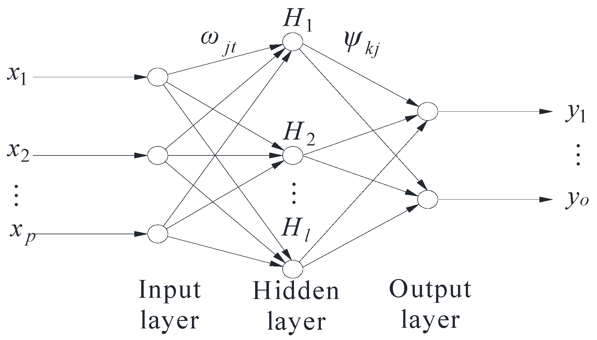
In this study, the transfer function for hidden layer neurons of the BPNN was selected as the S-type tangent function, while the transfer function for output layer neurons was chosen as the S-type logarithmic function. The Levenberg–Marquardt algorithm was employed for BPNN training and learning. The primary parameter settings for the genetic algorithm and BPNN are detailed in

Table 3. Main parameter settings of the genetic algorithm.

Number of Populations	50
Maximum number of generations	400
The number of binary digits of the variable	20
Generation gap	0.95
Probability of crossover	0.7
Probability of mutation	0.01

and

Table 4. Main parameter settings of the BPNN.

Maximum Training Times	1000
Momentum factor	0.9
Learning rate	0.1
Training goal	0.005

, respectively.

3.2. Cooling Load Prediction in the Early Cooling Stage

Using SPSS to process and analyze the sample data got the results of normal distribution detection of building cold load and its influencing factors at the early cooling stage, as shown in

Table 5. Normal distribution test results for the test data in the early cooing stage.

Indicators	Building Cooling Load and Its Influencing Factors
	Q	To	RHo	Io	Vo	Ti	RHi	Q(t − 1)
Average value	72.766 kW	29.013 °C	39.697%	476.889 W/m2	1.060 m/s	26.675 °C	43.249%	73.980 kW
Standard deviation	15.523 kW	4.123 °C	18.196%	238.526 W/m2	0.871 m/s	0.755 °C	12.712%	16.471 kW
Test statistic	0.147	0.041	0.156	0.061	0.124	0.051	0.098	0.146
Asymptotic significance	0.000	0.089	0.000	0.001	0.000	0.011	0.000	0.000

Note: Q(t − 1) represents the sequence of cooling loads at the previous moment (time interval of 0.5 h).

. The results of correlation analysis between building cold load and its influencing factors at the early cooling stage are shown in

Table 6. Correlation analysis between building cooling load and its influencing factors in the early cooling stage.

Indicator	Factors Affecting Building Cooling Loads
	To	RHo	Io	Vo	Ti	RHi	Q(t − 1)
Correlation coefficient	0.119 *	0.171 **	0.144 **	−0.129 **	0.221 **	0.180 **	0.956 **
Significance	0.014	0.000	0.003	0.008	0.000	0.000	0.000

Note: ** is used to indicate that two variables are significantly correlated at the 0.01 level. * is used to indicate that two variables are significantly correlated at the 0.05 level.

.

As shown in Table 5, only the asymptotic significance index of outdoor temperature was greater than 0.05 in the early cooling stage. It meant that only outdoor temperature obeyed the normal distribution.

As shown in Table 6, only the significance index of outdoor temperature was greater than 0.01, meaning that all parameters were significantly correlated with the building cooling load, except for outdoor temperature. This was because outdoor temperature was relatively low, which had a limited impact on the cooling load of the building in the early cooling stage. Therefore, outdoor relative humidity, solar radiation intensity, outdoor wind speed, indoor temperature, indoor relative humidity, and building cooling load at the previous moment were selected as the input variables of the prediction models in this cooling stage.

To evaluate the performance of the AIA prediction models improved by the sample similarity method, this study built eight contrast models. A comprehensive overview of different prediction models employed in the early cooling stage is provided in

Table 7. Detailed information on different prediction models in the early cooling stage.

Name	Main Input Variables	Detailed Description
M1	HRo; Io; Vo; Ti; RHi; Q(t − 1)	BPNN
M2	HRo; Io; Vo; Ti; RHi; Q(t − 1)	Similar samples screening +BPNN
M3	HRo; Io; Vo; Ti; RHi; Q(t − 1)	GABPNN
M4	HRo; Io; Vo; Ti; RHi; Q(t − 1)	Similar samples screening +GABPNN
M5	HRo; Io; Vo; Ti; RHi; Q(t − 1)	SVR neural network
M6	HRo; Io; Vo; Ti; RHi; Q(t − 1)	Similar samples screening +SVR neural network
M7	HRo; Io; Vo; Ti; RHi; Q(t − 1)	ELM neural network
M8	HRo; Io; Vo; Ti; RHi; Q(t − 1)	Similar samples screening +ELM neural network

.

The weight values for outdoor relative humidity, solar radiation intensity, outdoor wind speed, indoor temperature, indoor humidity and building cooling load at the previous moment were 0.1737, 0.1629, 0.1475, 0.1724, 0.1690, and 0.1745, respectively, calculated by the entropy weighting method. This study only selected historical samples with a comprehensive similarity coefficient greater than 0.6 as the similarity sample set.

The prediction results of different models in the early cooling stage are shown in Figure 11, Figure 12, Figure 13, Figure 14, Figure 15, Figure 16, Figure 17 and Figure 18. The APE distribution intervals of different prediction models are shown in Figure 19.

As shown in Figure 11, Figure 12, Figure 13, Figure 14, Figure 15, Figure 16, Figure 17, Figure 18 and Figure 19, the tendencies between the predicted and actual values of M1 to M8 were consistent. The APE of M1, M2, M3, M4, M5, M6, M7, and M8 was mainly distributed between 6.0 and 13.3%, 2.6 and 10.8%, 1.6 and 6.5%, 2.1 and 6.5%, 1.4 and 6.3%, 1.2 and 5.4%, 1.1 and 6.5%, and 1.7 and 7.5%, respectively. The prediction error of each model only exceeded 30% at certain moments. This was because the main operating mode of the soil source heat pump system in the early cooling stage was that the low-temperature water in the outdoor buried pipe heat exchanger was directly supplied to the indoor floor radiation coil system. However, sometimes the operating staff switched the cooling mode. Low-temperature water was directly supplied to the indoor fan coil. The instantaneous heat transfer capacity of the fan coil was greater than that of the floor radiation coil. It caused an instantaneous increase of the building cooling load (this study assumed that the measured instantaneous cooling load of the heat pump system reflected the building’s cooling load). When the terminal was switched to floor radiation cooling mode, it also caused an instantaneous decrease of the building cooling load. In addition, there was an overall higher prediction error on 20 June. It could be attributed to the elevated outdoor temperature on that date, leading to a larger building cooling load. However, the cooling load in the training samples was lower than the actual cooling load measured on 20 June. Consequently, the AIA faced challenges in training and learning effectively, resulting in a higher prediction error on that date.

The training and prediction errors of different models at the early cooling stage are shown in

Table 8. Evaluation of the prediction effect of different prediction models in the early cooling stage.

Model	Training Error			Prediction Error
	MAPE (%)	R2	RMSE (kW)	MAPE (%)	R2	RMSE (kW)
M1	3.7	0.892	4.092	11.5	0.535	14.611
M2	3.5	0.895	3.937	8.8	0.658	12.536
M3	2.6	0.917	3.593	7.2	0.632	12.992
M4	2.9	0.915	3.531	8.3	0.528	14.717
M5	2.2	0.908	3.777	5.4	0.811	9.319
M6	2.5	0.903	3.763	5.7	0.782	10.007
M7	2.8	0.903	3.889	6.4	0.742	10.881
M8	3.0	0.897	3.885	5.7	0.820	9.101

.

Table 8 provides insights into the cooling load predictions at the early cooling stage for M1 to M8. The training errors of M1 to M8 were relatively consistent. However, their prediction errors varied significantly. When the prediction models used the original data as the training samples, M5 yielded the best prediction accuracy, while the prediction accuracy of M1 was the worst. When the original data were pre-treated based on sample similarity, MAPE, R², and RMSE of M2 decreased from 11.5 to 8.8% (with a decrease of 23.5%), increased from 0.535 to 0.658 (with an increase of 23.0%), and decreased from 14.611 to 12.536 kW (with a decrease of 14.2%), respectively, compared to those of M1. It proves that the prediction accuracy of M2 had been greatly improved. Conversely, the MAPE, R², and RMSE of M4 increased from 7.2 to 8.3% (with an increase of 15.3%), decreased from 0.632 to 0.528 (with a decrease of 16.5%), and increased from 12.992 to 14.717 kW (with an increase 13.3%), respectively, compared to those of M3. It means that the prediction accuracy of the improved M4 had been decreased. The MAPE, R², and RMSE of M6 increased from 5.4 to 5.7% (with an increase of 5.6%), decreased from 0.811 to 0.782 (with a decrease of 3.6%), and increased from 9.319 to 10.007 kW (with an increase of 7.4%), respectively, compared to those of M5. The results of M6 were similar with those of M4, i.e., the prediction accuracy of M6 was decreased. M8 showed a substantial improvement, with its MAPE, R², and RMSE decreasing from 6.4 to 5.7% (with a decrease of 10.9%), increasing from 0.742 to 0.820 (with an increase of 10.5%), and decreasing from 10.881 to 9.101 kW (with a decrease of 16.4%), respectively, compared to those of M7.

3.3. Cooling Load Prediction in the Middle Cooling Stage

The outcomes of the normal distribution evaluation for the building’s cooling load and its impacting factors during the middle cooling stage are meticulously detailed in

Table 9. Normal distribution test results for the test data in the middle cooling stage.

Indicators	Building Cooling Load and Its Influencing Factors
	Q	To	RHo	Io	Vo	Ti	RHi	Q(t − 1)
Average value	169.105 kW	31.644 °C	62.727%	360.958 W/m2	0.690 m/s	25.078 °C	68.716%	168.599 kW
Standard deviation	53.664 kW	3.354 °C	15.966%	202.608 W/m2	0.543 m/s	0.380 °C	5.948%	53.055 kW
Test statistic	0.245	0.025	0.080	0.046	0.135	0.067	0.105	0.243
Asymptotic significance	0.000	0.200	0.000	0.003	0.000	0.000	0.000	0.000

Note: Q(t − 1) represents the sequence of cooling loads at the previous moment (time interval of 0.5 h).

. The results of the correlation analysis between the building’s cooling load and the pertinent factors for this cooling period are comprehensively expounded in

Table 10. Results of the correlation analysis between building cooling load and its influencing factors in the middle cooling stage.

Indicator	Factors Affecting Building Cooling Loads
	To	RHo	Io	Vo	Ti	RHi	Q(t − 1)
Correlation coefficient	0.427 **	−0.008	0.189 **	0.137 **	0.185 **	0.250 **	0.966 **
Significance	0.000	0.841	0.000	0.001	0.000	0.000	0.000

Note: ** is used to indicate that two variables are significantly correlated at the 0.01 level.

.

As shown in Table 9, only the asymptotic significance index of outdoor temperature was greater than 0.05 in the middle cooling stage. The asymptotic significance indexes of the rest of the influencing factors were 0. It means that only outdoor temperature obeyed the normal distribution, and the rest of the parameters did not obey the normal distribution.

As shown in Table 10, only the significance index of outdoor relative humidity was greater than 0.01, meaning that all parameters were significantly correlated with the building cooling load, except for outdoor relative humidity. It could be attributed to the limited dehumidification capacity of the soil source heat pump system. Changes of outdoor air relative humidity had a limited impact on the cooling load in the middle cooling stage. Therefore, outdoor temperature, solar radiation intensity, outdoor wind speed, indoor temperature, indoor relative humidity, and building cooling load at the previous moment were selected as the input variables of the prediction models in the middle cooling stage.

To evaluate the performance of the improved prediction model based on sample similarity, we built distinct control models for the middle cooling stage. Detailed specifications of the prediction models are provided in

Table 11. Detailed information on different prediction models for the middle cooling stage.

Name	Main Input Variables	Detailed Description
M1	To; Io; Vo; Ti; RHi; Q(t − 1)	BPNN
M2	To; Io; Vo; Ti; RHi; Q(t − 1)	Similar sample screening + BPNN
M3	To; Io; Vo; Ti; RHi; Q(t − 1)	GABPNN
M4	To; Io; Vo; Ti; RHi; Q(t − 1)	Similar sample screening + GABPNN
M5	To; Io; Vo; Ti; RHi; Q(t − 1)	SVR neural network
M6	To; Io; Vo; Ti; RHi; Q(t − 1)	Similar sample screening + SVR neural network
M7	To; Io; Vo; Ti; RHi; Q(t − 1)	ELM neural network
M8	To; Io; Vo; Ti; RHi; Q(t − 1)	Similar sample screening + ELM neural network

.

The weight values for the input parameters, including outdoor temperature, solar radiation intensity, outdoor wind speed, indoor temperature and relative humidity, and building cooling load at the previous moment were 0.1767, 0.1741, 0.1544, 0.1753, 0.1685, and 0.1510, respectively, calculated by the entropy weighting method. This study only selected historical samples with a comprehensive similarity coefficient greater than 0.6 as the similarity sample set.

The prediction results generated by various prediction models during the middle cooling stage are illustrated in Figure 20, Figure 21, Figure 22, Figure 23, Figure 24, Figure 25, Figure 26 and Figure 27. The APE distribution intervals of different prediction models are presented in Figure 28.

As shown in Figure 20, Figure 21, Figure 22, Figure 23, Figure 24, Figure 25, Figure 26, Figure 27 and Figure 28, when prediction of the cooling load during the middle cooling stage was conducted, a general consistency in the trend between predicted and actual values of M1 to M8 was observed. Specifically, the APE of M1 was primarily distributed within the range of 3.9 to 14.9%, while that of M2 was distributed within the range of 1.9 to 6.8%. The APE of M3 was primarily distributed within the interval of 0.7 to 2.5%, and for M4, the APE was distributed from 0.7 to 2.9%. The APE of M5 primarily ranged from 0.6 to 2.3%. The APE of M6 was mainly located between 0.6 and 2.1%. The APE of M7 was mainly distributed within the range of 0.9 to 3.5%. The APE of M8 was primarily located between 0.5 and 2.6%. The prediction error of each model only exceeded 30% at certain moments. This was because the main operating mode of the soil source heat pump system in this cooling stage was that heat pump A and B were combined for cooling. Sometimes the operating staff switched the working status of heat pumps A and B. The process of switching between heat pumps A and B required a certain amount of time to ensure system stability, which contributed to increasing prediction errors.

Table 12. Evaluation of the prediction effect of different prediction models in the middle cooling stage.

Model	Training Error			Prediction Error
	MAPE (%)	R2	RMSE (kW)	MAPE (%)	R2	RMSE (kW)
M1	7.6	0.889	15.641	10.5	0.850	25.580
M2	4.8	0.911	11.819	5.7	0.893	21.588
M3	2.7	0.963	9.020	2.8	0.903	20.574
M4	2.8	0.962	8.964	2.9	0.905	20.289
M5	2.2	0.967	8.508	2.6	0.905	20.370
M6	2.4	0.964	8.708	2.5	0.906	20.208
M7	2.7	0.964	8.961	3.3	0.904	20.467
M8	2.6	0.948	8.647	2.7	0.906	20.247

presents the training and prediction errors of different models in the middle cooling stage.

As shown in Table 12, when the original data were used as the training samples for the prediction models, the best prediction accuracy was obtained by M5, while the prediction accuracy of M1 was the worst. When the original data were pretreated using the sample similarity method, the MAPE, R², and RMSE of M2 decreased from 10.5 to 5.7% (with a reduction of 45.7%), increased from 0.850 to 0.893 (with an increase of 5.1%), and decreased from 25.580 to 21.588 kW (with a reduction of 15.6%), respectively, compared to that of M1. It means that the prediction accuracy of M2 had been greatly improved. R² and RMSE of M4 were improved compared to those of M3, while the MAPE got worse. The MAPE, R², and RMSE of M6 decreased from 2.6 to 2.5% (with a reduction of 3.8%), increased from 0.905 to 0.906 (with an increase of 0.1%), and decreased from 20.370 to 20.208 kW (with a reduction of 0.8%), respectively. It means that the prediction accuracy of M5 was slightly improved. MAPE, R², and RMSE of M8 decreased from 3.3 to 2.7% (with a reduction of 18.2%), increased from 0.904 to 0.906 (with an increase of 0.2%), and decreased from 20.467 to 20.247 kW (with a reduction of 1.1%), respectively, compared to those of M7. It proved that the prediction accuracy of M8 had been greatly improved.

In summary, the method of pretreating training samples based on sample similarity was highly effective in improving the prediction accuracy of BPNN and ELM models. However, this did not apply to GABPNN and SVR models. This was because the latter two neural networks inherently possess global optimization functions. The GABPNN utilizes the genetic algorithm to screen training samples, retaining the optimal individuals for network training. The SVR model ensures predictive accuracy through cross-validation for global validation. Excluding a part of the training samples makes it challenging to achieve global optimization in the training and learning of these two prediction models.

4. Conclusions and Future Works

In order to improve the accuracy of the conventional building cooling load prediction model based on an AIA, this paper proposes a training data selection method based on the similarity method. An office building located in Tianjin was selected as a case study. The main conclusions of this study are as follows:

(1) The impacts of outdoor temperature on the cooling load were different in the early and middle cooling stages. Due to the low outdoor temperature in the early cooling stage, its impact on building cooling load was not significant.

(2) When the original data were used as the training samples for conventional AIA prediction models, the best prediction accuracy was obtained by the SVR model, while the worst prediction accuracy was obtained by the BPNN model.

(3) For the developed BPNN model, the MAPE of decreased from 11.5 to 8.8%, R² increased from 0.535 to 0.658, and RMSE decreased from 14.611 to 12.536 kW in the early cooling stage. The MAPE of the developed BPNN model decreased from 10.5 to 5.7%, R² increased from 0.850 to 0.893, and RMSE decreased from 25.580 to 21.588 kW in the middle cooling stage. This demonstrated that the similarity sample screening method was suitable for the BPNN model.

(4) For the developed ELM model, the MAPE of the developed ELM model decreased from 6.4 to 5.7%, R² increased from 0.742 to 0.820, and RMSE decreased from 10.881 to 9.101 kW in the early cooling stage. The MAPE of the developed ELM model decreased from 3.3 to 2.7%, R² increased from 0.904 to 0.906, and RMSE decreased from 20.467 to 20.247 kW in the middle cooling stage. This demonstrated that the similarity sample screening method was suitable for the ELM model.

(5) The similarity sample screening method was not suitable for the GABPNN and SVR models, which inherently possess global optimization functions.

It is essential to acknowledge that this study is subject to limitations stemming from testing constraints, such as time and conditions. Economic and practical considerations of the developed AIA method were not considered either. The training sample data were received only from an office building in the summer, which resulted in a limited number of historical samples. Future research should be conducted to further validate the building load prediction accuracy (including heating load) of different AIA models improved by the similarity sample screening method for different types of buildings.

References

1. IEA. Energy Technology Perspective 2017; Catalysing Energy Technology Transformations: Paris, France, 2017. [Google Scholar]
2. Casals, X.G. Analysis of building energy regulation and certification in Europe: Their role, limitations and differences. Energy Build. 2006, 38, 381–392. [Google Scholar] [CrossRef]
3. Liu, Z.; Liu, Y.; He, B.; Xu, W.; Jin, G.; Zhang, X. Application and suitability analysis of the key technologies in nearly zero energy buildings in China. Renew. Sustain. Energy Rev. 2019, 101, 329–345. [Google Scholar] [CrossRef]
4. Al-Shargabi, A.A.; Almhafdy, A.; Ibrahim, D.M.; Alghieth, M.; Chiclana, F. Buildings’ energy consumption prediction models based on buildings’ characteristics: Research trends, taxonomy, and performance measures. J. Build. Eng. 2022, 54, 104577. [Google Scholar] [CrossRef]
5. Yuan, T.; Ding, Y.; Zhang, Q.; Zhu, N.; Yang, K.; He, Q. Thermodynamic and economic analysis for ground-source heat pump system coupled with borehole free cooling. Energy Build. 2017, 155, 185–197. [Google Scholar] [CrossRef]
6. Solano, J.C.; Caamaño-Martín, E.; Olivieri, L.; Almeida-Galárraga, D. HVAC systems and thermal comfort in buildings climate control: An experimental case study. Energy Rep. 2021, 7, 269–277. [Google Scholar] [CrossRef]
7. Wang, Y.; Li, Z.; Liu, J.; Zhao, Y.; Sun, S. A novel combined model for heat load prediction in district heating systems. Appl. Therm. Eng. 2023, 227, 120372. [Google Scholar] [CrossRef]
8. Yun, K.; Luck, R.; Mago, P.J.; Cho, H. Building hourly thermal load prediction using an indexed ARX model. Energy Build. 2012, 54, 225–233. [Google Scholar] [CrossRef]
9. Kwok, S.S.K.; Lee, E.W.M. A study of the importance of occupancy to building cooling load in prediction by intelligent approach. Energy Convers. Manag. 2011, 52, 2555–2564. [Google Scholar] [CrossRef]
10. Al-Shammari, E.T.; Keivani, A.; Shamshirband, S.; Mostafaeipour, A.; Yee, P.L.; Petković, D.; Ch, S. Prediction of heat load in district heating systems by support vector machine with firefly searching algorithm. Energy 2016, 95, 266–273. [Google Scholar] [CrossRef]
11. Sajjadi, S.; Shamshirband, S.; Alizamir, M.; Yee, P.L.; Mansor, Z.; Manaf, A.Z.; Altameem, T.A.; Mostafaeipour, A. Extreme learning machine for prediction of heat load in district heating systems. Energy Build. 2016, 122, 222–227. [Google Scholar] [CrossRef]
12. Leung, M.C.; Tse, N.C.F.; Lai, L.L.; Chow, T.T. The use of occupancy space electrical power demand in building cooling load prediction. Energy Build. 2012, 55, 151–163. [Google Scholar] [CrossRef]
13. Ilbeigi, M.; Ghomeishi, M.; Dehghanbanadaki, M. Prediction and optimization of energy consumption in an office building using artificial neural network and a genetic algorithm. Sustain. Cities Soc. 2020, 61, 102325. [Google Scholar] [CrossRef]
14. Fan, C.; Xiao, F.; Zhao, Y. A short-term building cooling load prediction method using deep learning algorithms. Appl. Energy 2017, 195, 222–233. [Google Scholar] [CrossRef]
15. Duanmu, L.; Wang, Z.; Zhai, Z.J.; Li, X. A simplified method to predict hourly building cooling load for urban energy planning. Energy Build. 2013, 58, 281–291. [Google Scholar] [CrossRef]
16. Yao, Y.; Lian, Z.; Liu, S.; Hou, Z. Hourly cooling load prediction by a combined forecasting model based on analytic hierarchy process. Int. J. Therm. Sci. 2004, 43, 1107–1118. [Google Scholar] [CrossRef]
17. Ding, Y.; Zhang, Q.; Yuan, T. Research on short-term and ultra-short-term cooling load prediction models for office buildings. Energy Build. 2017, 154, 254–267. [Google Scholar] [CrossRef]
18. Ren, C.; An, N.; Wang, J.; Li, L.; Hu, B.; Shang, D. Optimal parameters selection for BP neural network based on particle swarm optimization: A case study of wind speed forecasting. Knowl.-Based Syst. 2014, 56, 226–239. [Google Scholar] [CrossRef]
19. Zhang, Y.; Gao, X.; Katayama, S. Weld appearance prediction with BP neural network improved by genetic algorithm during disk laser welding. J. Manuf. Syst. 2015, 34, 53–59. [Google Scholar] [CrossRef]
20. Wang, H.; Jin, T.; Wang, H.; Su, D. Application of IEHO–BP neural network in forecasting building cooling and heating load. Energy Rep. 2022, 8, 455–465. [Google Scholar] [CrossRef]
21. Qian, L.; Zhao, J.; Ma, Y. Option Pricing Based on GA-BP neural network. Procedia Comput. Sci. 2022, 199, 1340–1354. [Google Scholar] [CrossRef]
22. Domashova, J.V.; Emtseva, S.S.; Fail, V.S.; Gridin, A.S. Selecting an optimal architecture of neural network using genetic algorithm. Procedia Comput. Sci. 2021, 190, 263–273. [Google Scholar] [CrossRef]
23. Oreski, S.; Oreski, G. Genetic algorithm-based heuristic for feature selection in credit risk assessment. Expert Syst. Appl. 2014, 41, 2052–2064. [Google Scholar] [CrossRef]
24. Sreenivasan, K.S.; Kumar, S.S.; Katiravan, J. Genetic algorithm based optimization of friction welding process parameters on AA7075-SiC composite. Eng. Sci. Technol. Int. J. 2019, 22, 1136–1148. [Google Scholar] [CrossRef]
25. Cortes, C.; Vapnik, V. Support-vector networks. Mach. Learn. 1995, 20, 273–297. [Google Scholar] [CrossRef]
26. Vapnik, V.N. The Nature of Statistical Learning Theory; Springer: New York, NY, USA, 1999; pp. 181–217. [Google Scholar]
27. Huang, G.B.; Zhu, Q.Y.; Siew, C.K. Extreme learning machine: A new learning scheme of feedforward neural networks. In Proceedings of the International Joint Conference on Neural Networks, Hungary, Budapest, 25–29 July 2004; pp. 985–990. [Google Scholar]
28. Huang, G.; Zhu, Q.; Siew, C. Extreme learning machine: Theory and applications. Neurocomputing 2006, 70, 489–501. [Google Scholar] [CrossRef]
29. Wang, T.; Lee, H. Developing a fuzzy TOPSIS approach based on subjective weights and objective weights. Expert Syst. Appl. 2009, 36, 8980–8985. [Google Scholar] [CrossRef]
30. Shannon, C.E. A mathematical theory of communication. Bell Syst. Tech. J. 1948, 27, 379–423. [Google Scholar] [CrossRef]
31. Sahoo, M.; Sahoo, S.; Dhar, A.; Pradhan, B. Effectiveness evaluation of objective and subjective weighting methods for aquifer vulnerability assessment in urban context. J. Hydrol. 2016, 541, 1303–1315. [Google Scholar] [CrossRef]
32. Analytical Methods Committee. Uncertainty of measurement: Implications of its use in analytical science. Analyst 1995, 120, 2303–2308. [Google Scholar] [CrossRef]
33. Akbulut, U.; Utlu, Z.; Kincay, O. Exergoenvironmental and exergoeconomic analyses of a vertical type ground source heat pump integrated wall cooling system. Appl. Therm. Eng. 2016, 102, 904–921. [Google Scholar] [CrossRef]
34. Hepbasli, A.; Akdemir, O. Energy and exergy analysis of a ground source (geothermal) heat pump system. Energy Convers. Manag. 2004, 45, 737–753. [Google Scholar] [CrossRef]
35. Chen, X.; Yang, H.; Lu, L.; Wang, J.; Liu, W. Experimental studies on a ground coupled heat pump with solar thermal collectors for space heating. Energy 2011, 36, 5292–5300. [Google Scholar]
36. Dai, L.; Li, S.; DuanMu, L.; Li, X.; Shang, Y. Experimental performance analysis of a solar assisted ground source heat pump system under different heating operation modes. Appl. Therm. Eng. 2015, 75, 325–333. [Google Scholar] [CrossRef]
37. Joint Committee for Guides in Metrology. Evaluation of Measurement Data-Guide to the Expression of Uncertainty in Measurement, JCGM 100:2008 (GUM 1995 with Minor Corrections); Bureau International des Poids et Mesures: Paris, France, 2010; pp. 1–20. [Google Scholar]
38. Moffat, R.J. Describing the uncertainties in experimental results. Exp. Therm. Fluid Sci. 1988, 1, 3–17. [Google Scholar] [CrossRef]
39. Guo, Q.; Tian, Z.; Ding, Y.; Zhu, N. An improved office building cooling load prediction model based on multivariable linear regression. Energy Build. 2015, 107, 445–455. [Google Scholar]
Figure 1. Structure of a typical three-layer BPNN.
Processes 11 03389 g001
Figure 2. BPNN learning flowchart.
Processes 11 03389 g002
Figure 3. Learning process of a GABPNN.
Processes 11 03389 g003
Figure 4. Structure of an SVR learning machine.
Processes 11 03389 g004
Figure 5. Flowchart for the calculation of the comprehensive similarity coefficient.
Processes 11 03389 g005
Figure 6. Prediction flow of AIA based on sample similarity improvement.
Processes 11 03389 g006
Figure 7. Variation curves of outdoor temperature and relative humidity.
Processes 11 03389 g007
Figure 8. Variation curves of solar radiation intensity and outdoor wind speed.
Processes 11 03389 g008
Figure 9. Measured change curve of cooling capacity of the heat pump system.
Processes 11 03389 g009
Figure 10. Variation curves of indoor temperature and relative humidity during the test period.
Processes 11 03389 g010
Figure 11. Comparison of predicted M1 values with actual values in the early cooling stage.
Processes 11 03389 g011
Figure 12. Comparison of predicted M2 values with actual values in the early cooling stage.
Processes 11 03389 g012
Figure 13. Comparison of predicted M3 values with actual values in the early cooling stage.
Processes 11 03389 g013
Figure 14. Comparison of predicted M4 values with actual values in the early cooling stage.
Processes 11 03389 g014
Figure 15. Comparison of predicted M5 values with actual values in the early cooling stage.
Processes 11 03389 g015
Figure 16. Comparison of predicted M6 values with actual values in the early cooling stage.
Processes 11 03389 g016
Figure 17. Comparison of predicted M7 values with actual values in the early cooling stage.
Processes 11 03389 g017
Figure 18. Comparison of predicted M8 values with actual values in the early cooling stage.
Processes 11 03389 g018
Figure 19. Distribution interval of APE of different prediction models in the early cooling stage.
Processes 11 03389 g019
Figure 20. Comparison of predicted M1 values with actual values in the middle cooling stage.
Processes 11 03389 g020
Figure 21. Comparison of predicted M2 values with actual values in the middle cooling stage.
Processes 11 03389 g021
Figure 22. Comparison of predicted M3 values with actual values in the middle cooling stage.
Processes 11 03389 g022
Figure 23. Comparison of predicted M4 values with actual values in the middle cooling stage.
Processes 11 03389 g023
Figure 24. Comparison of predicted M5 values with actual values in the middle cooling stage.
Processes 11 03389 g024
Figure 25. Comparison of predicted M6 values with actual values in the middle cooling stage.
Processes 11 03389 g025
Figure 26. Comparison of predicted M7 values with actual values in the middle cooling stage.
Processes 11 03389 g026
Figure 27. Comparison of predicted M8 values with actual values in the middle cooling stage.
Processes 11 03389 g027
Figure 28. Distribution interval of APE of different prediction models in the middle cooling stage.
Processes 11 03389 g028