Abstract
Response surface methodology (RSM) is one of the most effective design of experiments (DoE) methods for analyzing and optimizing experiments with limited data. However, the performance of RSM is highly dependent on the quality of the experimental data (e.g., measurement error and bias). In this work, we introduce a coefficient clipping technique based on prior knowledge to address this problem in RSM. To maintain the simplicity of RSM, the representative prior knowledge of monotonically increasing/decreasing and convex/concave relationships is considered as constraints. The proposed method uses the same experimental data as typical RSM, but can more accurately analyze the relationship between the independent variable and the output response. The performance of the proposed method is verified via various case studies, including the experiment of antibiotic adsorption in wastewater.
1. Introduction
The importance of achieving environmental sustainability and transitioning from fossil fuels to sustainable energy sources (e.g., renewable energy and hydrogen) has been increasingly emphasized due to industrial pollution and climate change [1,2,3,4,5]. Many research efforts have been devoted to the development of new technologies and materials [6,7,8,9,10,11,12,13]. In particular, technologies for environmental preservation and carbon neutrality face the need for rapid development and industrial validation due to various agreements and policy constraints (e.g., the Paris Agreement, net-zero scenarios [14]). However, traditional approaches that rely on extensive trial-and-error experimentation for process and material development have imposed significant time and cost constraints on rapid technology advancement. To address these challenges, many researchers are focusing on the design of experiments (DoE).
DoE is a powerful tool used in many fields of research to systematically design and conduct experiments [15,16,17]. It involves carefully selecting and controlling the variables of interest, manipulating their levels, and observing the output responses. DoE allows researchers to efficiently gather information and draw meaningful conclusions from limited experimental data. DoE has several advantages over traditional one-factor-at-a-time (OFAT) experiments [18]. First, it provides a better understanding of the system because multiple factors and their interactions can be studied simultaneously. This multi-factor approach allows researchers to uncover complex relationships and identify important factors that may have been missed in OFAT studies. Another advantage of DoE is its ability to optimize experimental resources. By strategically designing experimental conditions, DoE minimizes the number of experiments required while maximizing the information obtained. This efficiency allows researchers to save time, reduce costs, and explore a larger experimental space. Numerous studies have used DoE to address a variety of research questions and challenges. For instance, DoE has been used to optimize process parameters, improve product quality, and reduce manufacturing variability [19,20,21,22]. In pharmaceutical research, DoE has facilitated the development of drug formulations, optimized drug delivery systems, and identified critical process parameters [23,24]. Furthermore, in environmental research, DoE has supported treatment process optimization, source assessment, and environmental impact analysis [25,26]. The applications of DoE are not limited to specific disciplines; it is widely used in fields such as chemistry, engineering, agriculture, and the social sciences [27,28,29,30].
Response surface methodology (RSM) [31] is a statistical and mathematical technique commonly used in DoE. RSM aims to optimize and understand the relationship between the response variable of interest and the independent variables that influence it. The primary goal of RSM is to develop an empirical model that describes the behavior of the response variable within the experimental domain. This model is typically represented by a second-order polynomial that relates the response variable to the independent variables. RSM uses a series of designed experiments (Box–Behnken design; BBD, central composite design; CCD, Latin hypercube design; LHD) to collect data from different combinations of factor levels. These experiments are strategically designed to explore the factor space efficiently, maximizing the information gained while reducing the number of experiments required. Once the experimental data are collected, regression analysis is used to estimate model parameters. The estimated model can then be used to predict response variables under different conditions, understand the relationship between factors and responses, and identify optimal conditions. Because the method is intuitive and requires minimal experimentation, it is widely used to optimize experiments in various fields, including chemical, mechanical, biological, environmental, and pharmaceutical areas [32,33,34,35,36,37,38].
However, the accuracy and availability of limited and biased experimental data can significantly affect the quality of the estimated model, resulting in a model that behaves differently to the actual system. Previous research on improving the performance of RSMs has proposed methodologies for designing and conducting additional experiments to address these issues. However, these methods require additional experiments, which inevitably incur time and monetary costs. The present study introduces a new approach for improving the performance of response surface methodology (RSM) while using the same amount of data as previous methods. The proposed method incorporates a coefficient clipping technique that imposes constraints on the estimation of model coefficients by utilizing prior knowledge derived from physical and chemical properties or preliminary experiments. By integrating this prior knowledge, the proposed method improves the estimation performance of the RSM model. Two simple scenarios are considered: when the independent variable has a monotonic relationship with the output response and when it has a convex or concave relationship. Constraints from these scenarios ensure that the quadratic form of the RSM model satisfies specific properties within the range of the independent variables. The effectiveness of the proposed method is demonstrated through case studies, including the optimization of antibiotic adsorption experiments, where it outperforms existing methods.
2. Materials and Methods
Response surface methodology (RSM) is used in conjunction with experimental designs such as Box–Behnken design (BBD) and central composite design (CCD) to analyze and optimize complex interactions present in experiments by approximating them with a simple model. The most commonly used mathematical form is the second-order polynomial [31], which can be expressed as follows:
Here, and denote the independent variables and the output response, respectively. represents the model coefficients, and k is the number of independent variables. In Equation (1), each term on the right-hand side represents the bias (), the independent effect of the variable (), the correlation between the variables (), and the curvature effect of the variable (), in that order. Although it is a simple second-order polynomial, it effectively explains the behavior of experiments with limited measurement data. However, the second-order model may not always provide accurate analysis results due to uncontrollable measurement errors and highly complex relationships between independent variables and output responses.
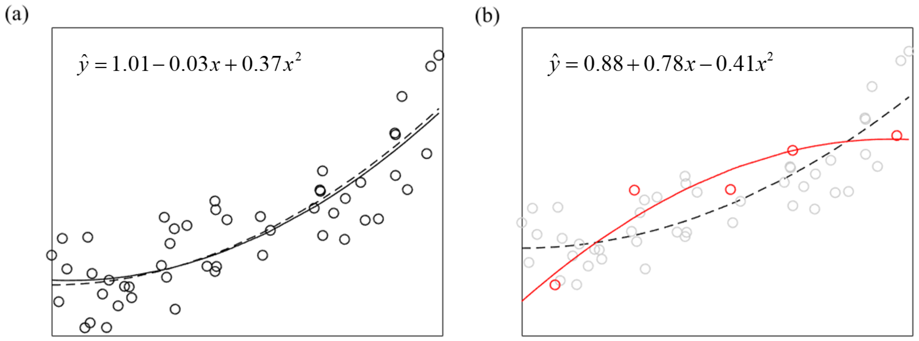
Biased and inadequate experimental data can significantly affect the accuracy and availability of estimated models, potentially resulting in models that describe behavior different from the actual system. The results of a model regression using an arbitrary second-order model of with measurement errors are shown in Figure 1. As shown in Figure 1, experimental data often contain unavoidable measurement errors. Figure 1a shows that, with a larger number of repeated measurements, it is possible to estimate a more accurate model with minimal impact from measurement errors. In contrast, when the data are limited and biased by measurement errors, the estimated model may behave differently (represented by the solid line in Figure 1b) to the actual behavior (represented by the dashed line in Figure 1b). Collecting more data can improve the estimation performance of RSM models by reducing the impact of measurement error. However, this approach contradicts the purpose of using DoE. To overcome this, this study proposes a new approach that utilizes prior knowledge to improve model performance while using the same amount of data as in previous methods.
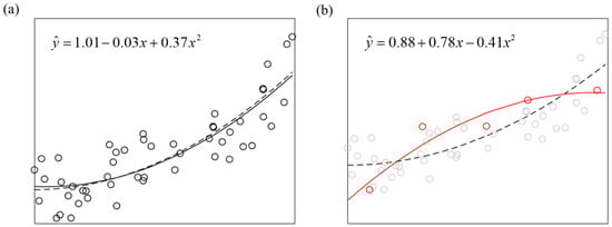
Figure 1.
Representative example showing the second-order polynomial regression (circle: measured data, solid line: regressed model, and dashed line: true model); (a) well-estimated model and (b) wrongly estimated model (red remarked data are only considered).
The proposed method uses the coefficient clipping approach, which applies constraints to the coefficient estimation of the model using prior knowledge from physical and chemical properties or preliminary experiments. To maintain the simplicity and accessibility of the second-order polynomial RSM model, the proposed method is designed for two circumstances where information is generally accessible and expressed as constraints.
Prior knowledge about the experiment is represented by derivatives of Equation (1) and is considered as a constraint on the model coefficient estimation problem. The study considers two commonly observed tendencies in the relationship between independent variables and output responses: monotonic and convex/concave relationships. In the case of a monotonic relationship, the derivative value for the output response is positive for a monotonically increasing relationship with the independent variable, while it is negative for a monotonically decreasing relationship. The convex or concave relationship between the independent variables and the output response is observed when the output response reaches its maximum or minimum value within the range of the independent variables. In this case, the output response reaches its maximum or minimum value at a specific point of the independent variable that satisfies Equation (6). Within the range of the independent variables, the following properties must be satisfied because the model for RSM is quadratic. The constraints for both cases can be represented as follows:
Monotonic relationship
For a monotonic increasing relationship:
For a monotonic decreasing relationship:
Convex and concave relationship
This equation can be rewritten as:
where subscript and are lower and upper bounds. Then, Equation (6) can be represented as the following linear constraints.
By clipping the associated coefficient, it is possible to improve the estimation performance of the RSM model.
3. Result and Discussion
Simulation and experimental studies are performed to verify the proposed methods. To solve the constraint regression problem of both methods, MATLAB fmincon function is used.
3.1. Case 1: One-Variable Experiment with a Factorial Design
The first example shows the performance of the proposed method by performing a simulation using an arbitrary function with one variable (, represented earlier in Figure 1) as a fictitious experiment. The quadratic function was used as the true relationship between the independent variable (X) and the output response (Y) with X ranging from 0 to 1, and three to seven equally spaced levels of the factorial design. The output response is generated by simulation. Here, the output response is interrupted by measurement error. The magnitude of measurement error is assumed as 5%, 10%, and 20%, respectively. The measurement errors were simulated using uniformly distributed random numbers between 0 and 1. The study performed 10,000 separate RSMs and calculated the average of their mean square error (MSE) to compare the performance of the proposed method with the previous approaches. In this example, it was assumed that the researcher has prior knowledge that the output response has a convex and monotonically increasing behavior with respect to the independent variable. Based on this, the RSM model and constraints used in this example were as follows:
s.t.
Table 1 compares the percentage of incorrectly estimated models and the MSE values for each scenario between the previous and proposed methods. In this example, wrong behavior was assumed to be any model that did not satisfy the prior knowledge of the convex relationship between the independent variable and the output response. As shown in Table 1, the previous method was more likely to estimate models that did not follow the true behavior, especially when the number of measurements was small and the measurement error was significant. When the measurement error was 20%, which is common in some applications such as biological and wastewater experiments, the previous method estimated models with concave behavior (i.e., opposite to the original convex behavior) for about 25–30% of the repeated simulation. In contrast, the proposed method incorporated additional constraints and was able to estimate the true behavior even under measurement errors, with significantly lower MSE values overall.

Table 1.
Performance of the proposed coefficient clipping method in Case 1.
3.2. Case 2: Two-Variable RSM Using Vehicle Miles per Gallon (MPG) Data
In this case study, the proposed method was validated using a data set on vehicle characteristics and fuel economy, which is widely used as an example of a regression problem. It was obtained from Quinlan’s paper [39]. The data set has diverse variables related to fuel economy. Among the variables in the entire data set, the weight () and horsepower () of the vehicle were set as the independent variables and MPG as the output response (Y) in this study. The RSM model used was:
In the relationship between vehicle characteristics and fuel economy, it was known that the weight of a vehicle has a monotonically decreasing relationship with fuel economy, so the proposed method additionally used the following constraint:
The relationships between MPG and the independent variables of previous and proposed methods were given by Equations (9) and (10), respectively.
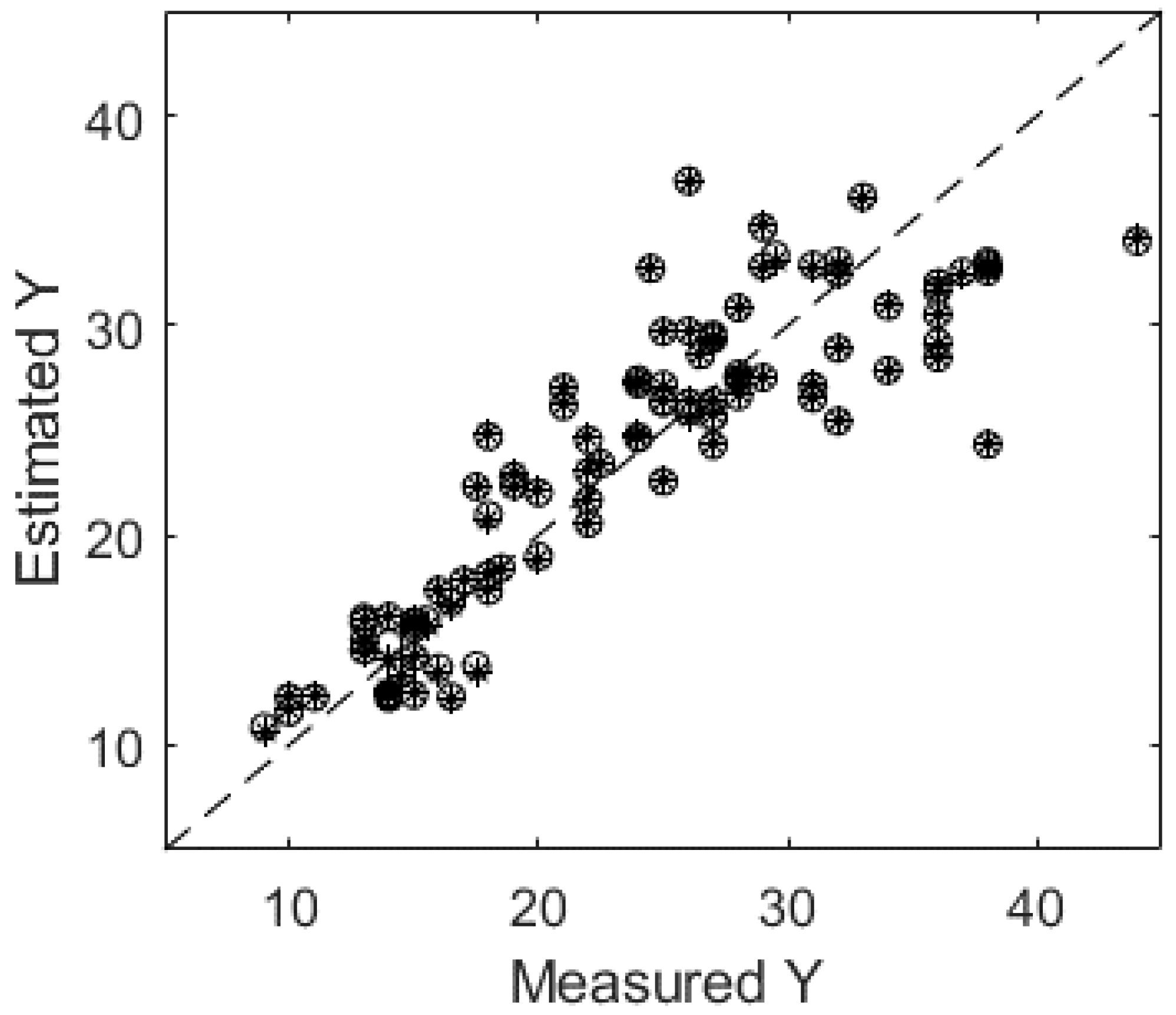
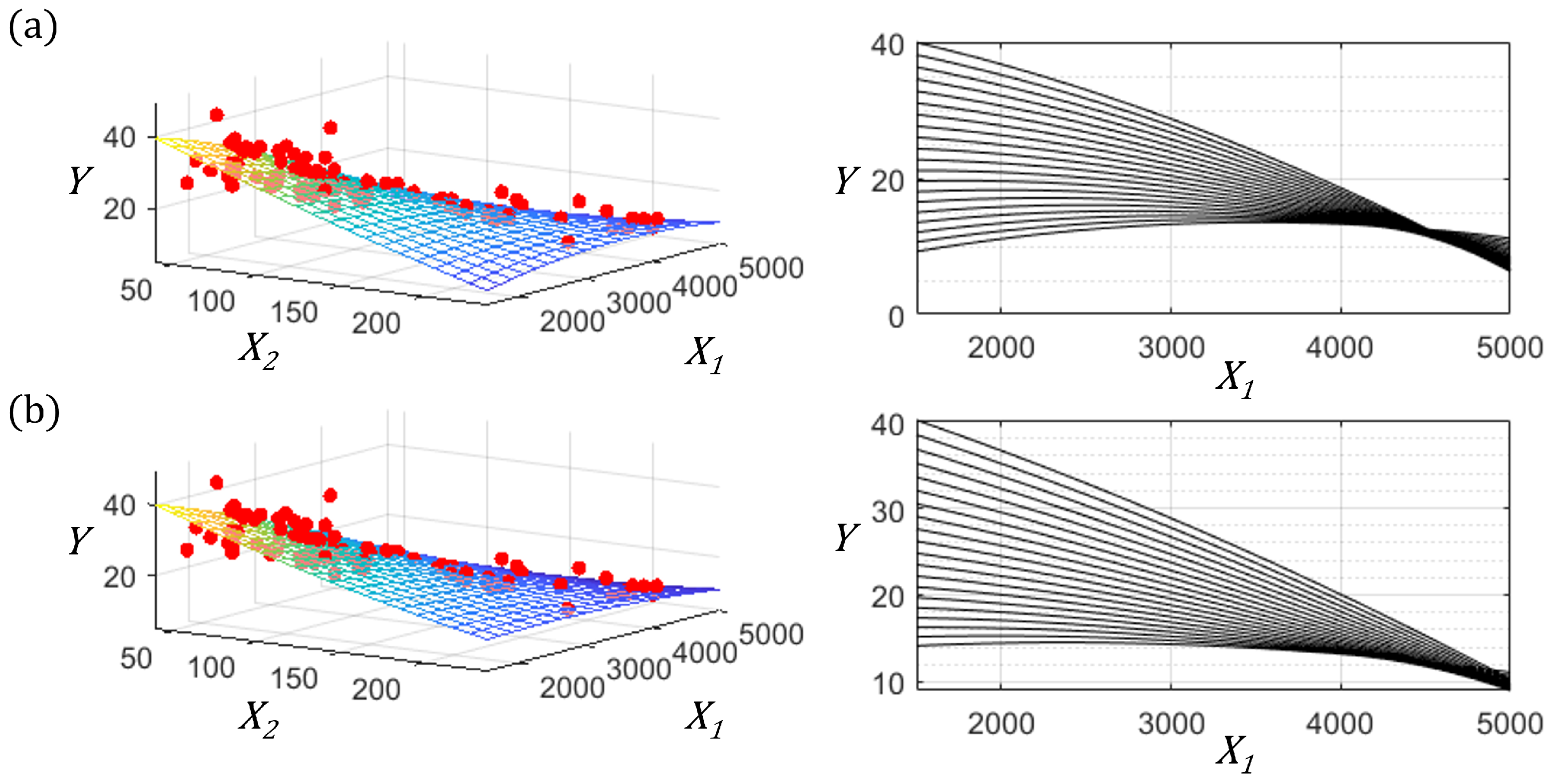
In contrast to Case 1, the data points of independent variables are unevenly distributed across the bins. The fuel economy data have a relatively unbalanced data set with relatively little data in the light weight–high horsepower and heavy weight–low horsepower regions. As shown in Figure 2, the MPG fitting results of the previous and proposed methods show similar performance with little difference. In Figure 3, the left graph is a 3D plot showing the relationship between the estimated model (mesh) and the data used for estimation (red circle). In this figure, it can be confirmed that both methods describe the relationship between vehicle information (: weight and : horsepower) and MPG similarly, but when checking the MPG estimation result for vehicle weight on the right side of the plot, the existing method tends to estimate the result value different from the actual trend, which is that the MPG increases rather than decreases with the weight of the vehicle. On the other hand, the proposed method explains the existing relationship between weight and MPG well. Although the model fitting results of the proposed method and the previous method could be similar depending on the data used, the proposed method shows the possibility of estimating RSM models for further applications (e.g., optimization) even with a relatively unbalanced distribution of the data used in the regression.
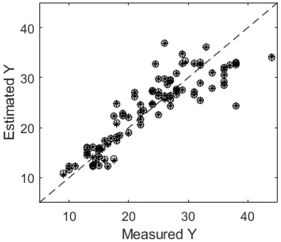
Figure 2.
Comparative result of output response prediction performance (star mark: from the previous method, and circle: from the proposed method).
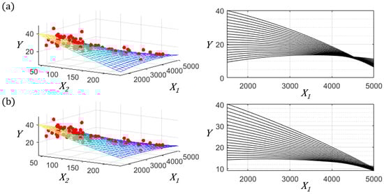
Figure 3.
Comparative results of output response with respect to independent variables; (a) the previous method and (b) the proposed method. (red circle: obtained data and meshed line: got response surface).
3.3. Case 3: Searching Optimal Experimental Conditions for Antibiotics Adsorption Using Thermal Treated Activated Carbon
In Case 3, the study conducted the wastewater treatment experiment. The proposed method is applied to this experiment to optimize the removal of tetracycline (TC) from aqueous solutions by simultaneously determining the properties of the adsorbent and the operating conditions. This experiment considers the treatment of powdered activated carbon (PAC) and adsorption experiment conditions as a significant independent variable.
First, select the heat treatment temperature as the independent variable. Exposing PAC to high temperatures can cause physical and chemical changes in PAC that can lead to the formation of new surface functional groups and changes in pore structure, which can improve the performance of the PAC. In general, careful control of heat treatment conditions, such as temperature, can tailor the properties of activated carbon to optimize its performance as an adsorbent for specific pollutants.
It is widely known that experimental conditions in adsorption experiments, such as pH and ionic strength, are highly associated with adsorption efficiency and selectivity. These parameters affect the electrostatic interactions between the antibiotic molecules and the adsorbent surfaces, as well as the distribution and stability of the antibiotic solution. Thus, pH and ionic strength in the adsorption experiment are also selected as independent variables. Consequently, three independent variables are considered, including heat treatment temperature, pH, and ionic strength.
For this experiment, coconut-shell-based PAC was purchased from Samchully Activated Carbon Co, Ltd. (Seoul, Republic of Korea). The 38–72 PAC size was separated by sieving and then treated with 0.05 M hydrochloric acid solution to remove soluble salts and other impurities (e.g., metals) that could affect the adsorption properties. The acid-treated PAC was washed with ultrapure water and dried at 150 degrees Celsius for 12 h. PAC was thermally treated under argon gas in the temperature range of 500 to 900 degrees Celsius to improve its adsorption properties. Potassium nitrate (KNO, 99.0% by weight) was used to manipulate the ionic strength, and sodium hydroxide (NaOH, 97% by weight) and hydrochloric acid (HCl, 37% by weight) were used to control the pH. All chemicals, including tetracycline hydrochloride (CHNO-HCl; TC-HCl), were purchased from Merck KGaA (Darmstadt, Germany) and were guaranteed to be of analytical grade and used as received.
A TC stock solution of 1000 mg/L was prepared by dissolving TC-HCl in ultrapure water. Batch equilibrium adsorption experiments were performed at room temperature in 40 mL conical tubes. Heat-treated PAC (from 500 to 900 degrees Celsius) at 0.02 g each was dispersed in ultrapure water, and KNO was dissolved to achieve the desired ionic strength. The pH was adjusted using aqueous HCl and NaOH solutions at 0.1 N. Each prepared sample had a total volume of 40 mL. The specific conditions, including PAC heat treatment temperature, KNO concentration, and pH, for each sample are summarized in Table 2. The prepared samples were shaken in a water bath shaker (DS-250SW, Daewon Science, Inc., Cheongju, Republic of Korea) at 150 rpm for 4 h at 396.15 K, and then the samples were filtered through a 0.45 polyvinylidene fluoride (PVDF) filter. The amount of TC adsorbed per PAC (Y, mgTC/gPAC) was calculated using the following formula:
Table 2.
Experimental range and levels of independent variables.
Here, , , and represent the initial tetracycline concentration, the tetracycline concentration of the i-th sample after adsorption, and the weight of the adsorbent used, respectively. In this study, all data were collected in triplicate, and averages were reported.
In Case 3, RSM was used to optimize the removal of TC from an aqueous solution. First, an inscribed type of central composite design (CCD) was used to obtain sufficient information from the experiment with a minimum number of experiments. The coded values and ranges of the experimental variables are listed in Table 2. To describe the output response in relation to the independent variables, a quadratic model formula was used as follows:
where is the predicted amount of TC absorbed, and , , and are the thermal treatment temperature, pH, and ionic strength, respectively. The response surface model of Equation (14) was fitted using both the previous and proposed methods. Optimization was then performed using the amount of TC absorbed as the objective function, reflecting the adsorption process’s efficiency. The optimal conditions were determined by maximizing the objective function while ensuring that the constraints on the decision variables were met using the fmincon function in MATLAB. The experimental results obtained from the iterative experiments are summarized in Table 3.
Table 3.
Experimental conditions and results using an inscribed type of central composite design.
In this case, it was preliminarily known that the relationship between PAC heat treatment temperature () and adsorbed TC per PAC is concave, and the ionic strength () monotonically decreases the adsorption performance. Therefore, the proposed method additionally considered the following constraints.
An empirical relationship between the tetracycline adsorption amount () and the decision variables is described by the previous method of Equation (18) and the proposed method of Equation (19) as follows:
Previous method
Proposed method
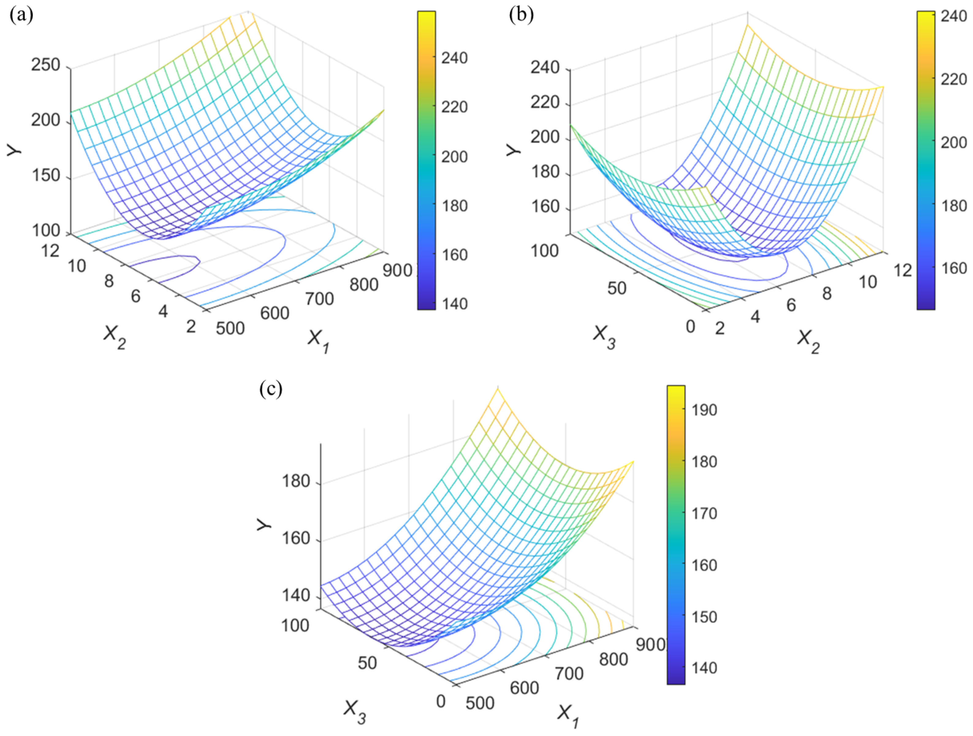
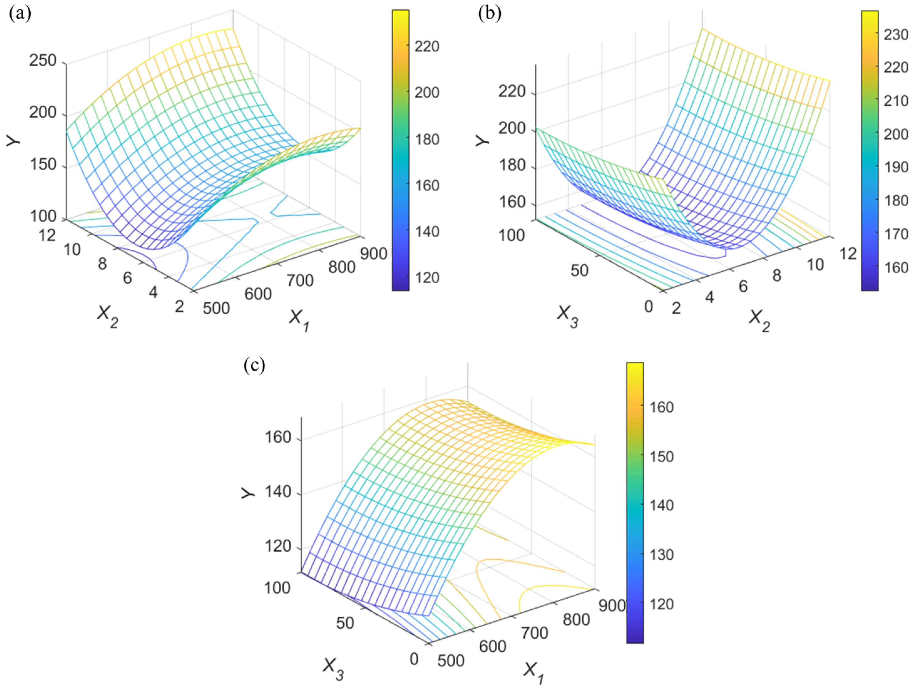
Figure 4 and Figure 5 represent the results plotted for the previous and proposed methods, respectively. Overall, they show similar trends, but it can be observed that the tendency of the thermal treatment temperature of the activated carbon is opposite. As previously reported in the literature, the thermal treatment of activated carbon tends to increase the adsorption capacity of antibiotics with an increasing temperature. However, it decreases when the thermal treatment temperature becomes too high. This is commonly attributed to pore contraction or carbon loss at high temperatures, resulting in a decrease in active sites and surface area. However, as shown in Figure 4, which was obtained using the previous method, the model represents the behavior of TC adsorption in PAC with respect to thermal treatment in a monotonically increasing form, which is believed to be due to modeling errors caused by experimental measurement uncertainties. On the other hand, the proposed method, as shown in Figure 5, captures the model that shows the same trend as previously reported studies and preliminary experiments. By solving the problem of TC adsorption optimization using the respective models, the optimal conditions and predicted adsorption capacities are as follows:
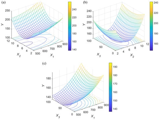
Figure 4.
Three−dimensional surface and contour plot of the previous method illustrating interaction between (a) heat treatment temperature, pH, and TC adsorption, (b) pH, ionic strength, and antibiotic adsorption, and (c) heat treatment temperature, ionic strength, and TC adsorption.
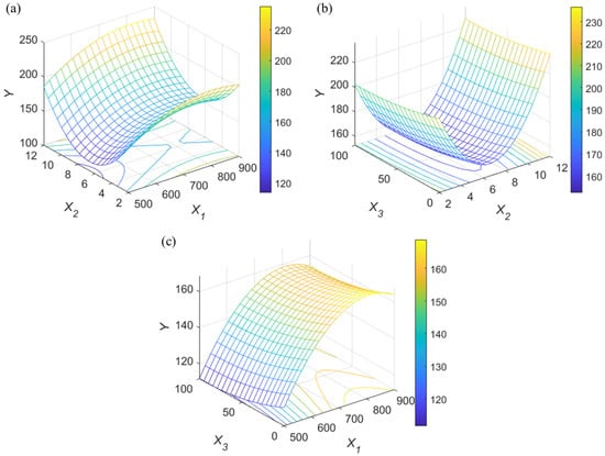
Figure 5.
Three−dimensional surface and contour plot of the proposed method illustrating interaction between (a) heat treatment temperature, pH, and TC adsorption, (b) pH, ionic strength, and antibiotic adsorption, and (c) heat treatment temperature, ionic strength, and TC adsorption.
Previous method
C, , mM, and mgTC/gPAC
Proposed method
C, , mM, and mgTC/gPAC
The methods predicted the optimum TC adsorption of 269.1 and 243.5 mgTC/gPAC at different of 900 and 816 degrees Celsius, respectively. The optimal heat treatment temperature of the proposed method was adjusted to 800 C since the heat treatment temperature difference of 16 C was not significant. The obtained optimum experiments were performed, and both methods experimentally obtained TC adsorption results of 228.2 mgTC/gPAC (optimum in the typical RSM method) and 247.5 mgTC/gPAC (optimum in the proposed method), respectively. The conventional method showed a significant difference (17.9% overestimated) between the adsorption amount predicted by the optimization and the actual results, which resulted in lower adsorption results than data obtained from CCD. This shows that the existing method needs to analyze the actual behavior better when the measurement data contain errors. On the other hand, the proposed method shows that the estimated optimization value is similar to the actual experiment (1.6% underestimated) and yields better adsorption results. This confirms that the proposed method can use constraints based on prior knowledge to estimate a response surface model that can better represent the experiment using the same experimental data and has good predictive performance when used to optimize the experiment.
4. Conclusions
DoE is widely used to estimate relationships between experimental variables with limited information and to optimize experiments using this information. These methods make use of limited experimental data, which often contain measurement errors. The quality of model estimation can be affected by the availability and accuracy of the data, especially when the data are limited and biased, resulting in an estimation of models that represent different behavior to the actual behavior.
To overcome these problems, the present study proposes a new approach for improving the predictive performance of response surface methodology (RSM) models while maintaining the amount of data used by previous RSM methods. In this study, a second-order polynomial model, which can be easily estimated using the least squares method, is set as the RSM model. The proposed method introduces a coefficient clipping approach to add constraints to the estimation of variables based on prior knowledge obtained from physical and chemical properties or previous experiments. By utilizing this prior knowledge, the proposed method can improve the estimation performance of the model while using the same data as before. The proposed method considers two situations: when the independent variable has a monotonic relationship with the output response and when the independent variable has a convex or concave relationship with the output response. These constraints ensure that the considered RSM model with a quadratic form satisfies certain properties within the range of independent variables. The performance of the proposed method is validated through various case studies. The proposed method is applied to the optimization of actual antibiotic adsorption experiments and is found to outperform the existing methods. The optimal value found by the proposed method has a higher prediction accuracy (1.6% error) than that of the existing method, and it can be confirmed that the adsorption amount is excellent (247.5 mgTC/gPAC). The proposed method can effectively describe the behavior of the system and find the optimal independent variables while maintaining the method’s simplicity and minimal number of required experiments, which is expected to be widely used in various fields, such as the optimization of experiments related to the synthesis and production of various materials, as well as the design of processes and finding of operating conditions. In addition, the method is highly applicable because it can be directly applied to studies that have already utilized RSM using the same data.
The proposed method showed the ability to adequately represent the relationship between independent variables and output responses using limited experimental data, which can be used for dynamics analysis and optimization of experiments. However, the RSM method based on second-order polynomials has a structurally symmetric behavior near the optimum point. Since the relationship between some independent variables and the output response may be convergent or stiffly varying around the optimum, the RSM method must be improved to apply a diverse experimental system.
Author Contributions
Conceptualization, K.H.R.; Methodology, K.H.R.; Software, J.K.; Validation, J.K. and D.-G.K.; Investigation, D.-G.K.; Data curation, D.-G.K.; Writing—original draft, J.K. and K.H.R.; Supervision, K.H.R.; Funding acquisition, K.H.R. All authors have read and agreed to the published version of the manuscript.
Funding
This work was supported by the Ministry of Education of the Republic of Korea and the National Research Foundation of Republic of Korea (RS-2023-00252445).
Data Availability Statement
The data presented in this study are available upon request from the corresponding author. However, data from the Quinlan study are available in a publicly accessible repository: (https://archive.ics.uci.edu/dataset/9/auto+mpg).
Conflicts of Interest
The authors declare no conflict of interest.
References
- Tian, J.; Yu, L.; Xue, R.; Zhuang, S.; Shan, Y. Global low-carbon energy transition in the post-COVID-19 era. Appl. Energy 2022, 307, 118205. [Google Scholar] [CrossRef]
- Kovač, A.; Paranos, M.; Marciuš, D. Hydrogen in energy transition: A review. Int. J. Hydrogen Energy 2021, 46, 10016–10035. [Google Scholar] [CrossRef]
- Kamyab, H.; Klemeš, J.J.; Van Fan, Y.; Lee, C.T. Transition to sustainable energy system for smart cities and industries. Energy 2020, 207, 118104. [Google Scholar] [CrossRef]
- Wang, S.; Sun, L.; Iqbal, S. Green financing role on renewable energy dependence and energy transition in E7 economies. Renew. Energy 2022, 200, 1561–1572. [Google Scholar] [CrossRef]
- Muntasir, M.; Zahoor, A.; Shabbir, A.M.; Haider, M.; Rehman, A.; Vishal, D. Reinvigorating the role of clean energy transition for achieving a low-carbon economy: Evidence from Bangladesh. Environ. Sci. Pollut. Res. 2021, 28, 67689–67710. [Google Scholar]
- Zagho, M.M.; Hassan, M.K.; Khraisheh, M.; Al-Maadeed, M.A.A.; Nazarenko, S. A review on recent advances in CO2 separation using zeolite and zeolite-like materials as adsorbents and fillers in mixed matrix membranes (MMMs). Chem. Eng. J. Adv. 2021, 6, 100091. [Google Scholar] [CrossRef]
- Al-Mamoori, A.; Krishnamurthy, A.; Rownaghi, A.A.; Rezaei, F. Carbon capture and utilization update. Energy Technol. 2017, 5, 834–849. [Google Scholar] [CrossRef]
- Lee, J.; Lee, W.; Ryu, K.H.; Park, J.; Lee, H.; Lee, J.H.; Park, K.T. Catholyte-free electroreduction of CO2 for sustainable production of CO: Concept, process development, techno-economic analysis, and CO2 reduction assessment. Green Chem. 2021, 23, 2397–2410. [Google Scholar] [CrossRef]
- Gür, T.M. Review of electrical energy storage technologies, materials and systems: Challenges and prospects for large-scale grid storage. Energy Environ. Sci. 2018, 11, 2696–2767. [Google Scholar] [CrossRef]
- Wilcox, J.; Psarras, P.C.; Liguori, S. Assessment of reasonable opportunities for direct air capture. Environ. Res. Lett. 2017, 12, 065001. [Google Scholar] [CrossRef]
- Dieterich, V.; Buttler, A.; Hanel, A.; Spliethoff, H.; Fendt, S. Power-to-liquid via synthesis of methanol, DME or Fischer–Tropsch-fuels: A review. Energy Environ. Sci. 2020, 13, 3207–3252. [Google Scholar] [CrossRef]
- Lee, W.J.; Li, C.; Prajitno, H.; Yoo, J.; Patel, J.; Yang, Y.; Lim, S. Recent trend in thermal catalytic low temperature CO2 methanation: A critical review. Catal. Today 2021, 368, 2–19. [Google Scholar] [CrossRef]
- Olabi, A.; Onumaegbu, C.; Wilberforce, T.; Ramadan, M.; Abdelkareem, M.A.; Al-Alami, A.H. Critical review of energy storage systems. Energy 2021, 214, 118987. [Google Scholar] [CrossRef]
- IEA. World Energy Outlook 2022; IEA: Paris, France, 2022. [Google Scholar]
- Fisher, R.A. Design of experiments. Br. Med. J. 1936, 1, 554. [Google Scholar] [CrossRef]
- Durakovic, B. Design of experiments application, concepts, examples: State of the art. Period. Eng. Nat. Sci. 2017, 5, 421–439. [Google Scholar] [CrossRef]
- Kim, B.; Ryu, K.H.; Heo, S. Mean squared error criterion for model-based design of experiments with subset selection. Comput. Chem. Eng. 2022, 159, 107667. [Google Scholar] [CrossRef]
- Frey, D.D.; Engelhardt, F.; Greitzer, E.M. A role for “one-factor-at-a-time” experimentation in parameter design. Res. Eng. Des. 2003, 14, 65–74. [Google Scholar] [CrossRef]
- Karacan, F.; Ozden, U.; Karacan, S. Optimization of manufacturing conditions for activated carbon from Turkish lignite by chemical activation using response surface methodology. Appl. Therm. Eng. 2007, 27, 1212–1218. [Google Scholar] [CrossRef]
- Saari, N.; Lamaming, J.; Hashim, R.; Sulaiman, O.; Sato, M.; Arai, T.; Kosugi, A.; Nadhari, W.N.A.W. Optimization of binderless compressed veneer panel manufacturing process from oil palm trunk using response surface methodology. J. Clean. Prod. 2020, 265, 121757. [Google Scholar] [CrossRef]
- Geng, H.; Xiong, J.; Huang, D.; Lin, X.; Li, J. A prediction model of layer geometrical size in wire and arc additive manufacture using response surface methodology. Int. J. Adv. Manuf. Technol. 2017, 93, 175–186. [Google Scholar] [CrossRef]
- Jiang, N.; Zhao, Y.; Qiu, C.; Shang, K.; Lu, N.; Li, J.; Wu, Y.; Zhang, Y. Enhanced catalytic performance of CoOx-CeO2 for synergetic degradation of toluene in multistage sliding plasma system through response surface methodology (RSM). Appl. Catal. B Environ. 2019, 259, 118061. [Google Scholar] [CrossRef]
- Shah, S.N.H.; Asghar, S.; Choudhry, M.A.; Akash, M.S.H.; Rehman, N.u.; Baksh, S. Formulation and evaluation of natural gum-based sustained release matrix tablets of flurbiprofen using response surface methodology. Drug Dev. Ind. Pharm. 2009, 35, 1470–1478. [Google Scholar] [CrossRef]
- Bhattacharya, S. Central composite design for response surface methodology and its application in pharmacy. In Response Surface Methodology in Engineering Science; IntechOpen: London, UK, 2021. [Google Scholar]
- Gengec, E.; Kobya, M.; Demirbas, E.; Akyol, A.; Oktor, K. Optimization of baker’s yeast wastewater using response surface methodology by electrocoagulation. Desalination 2012, 286, 200–209. [Google Scholar] [CrossRef]
- Salah Al-Shati, A.; Alabboodi, K.O.; Shamkhi, H.A.; Abd, Z.N.; Emeen, S.I.M. The Treatment of Hospital Wastewater Using Electrocoagulation Process—Analysis by Response Surface Methodology. J. Ecol. Eng. 2023, 24, 260–276. [Google Scholar] [CrossRef]
- Zhdanova, L.; Lucas, T. Justice beliefs, personal well-being and harsh social attitudes: Initial demonstration of a polynomial regression and response surface methodology. Curr. Psychol. 2016, 35, 615–624. [Google Scholar] [CrossRef]
- Humberg, S.; Nestler, S.; Back, M.D. Response surface analysis in personality and social psychology: Checklist and clarifications for the case of congruence hypotheses. Soc. Psychol. Personal. Sci. 2019, 10, 409–419. [Google Scholar] [CrossRef]
- Askari, M.; Abbaspour-Gilandeh, Y.; Taghinezhad, E.; El Shal, A.M.; Hegazy, R.; Okasha, M. Applying the response surface methodology (RSM) approach to predict the tractive performance of an agricultural tractor during semi-deep tillage. Agriculture 2021, 11, 1043. [Google Scholar] [CrossRef]
- Yolmeh, M.; Jafari, S.M. Applications of response surface methodology in the food industry processes. Food Bioprocess Technol. 2017, 10, 413–433. [Google Scholar] [CrossRef]
- Myers, R.H.; Montgomery, D.C.; Anderson-Cook, C.M. Response Surface Methodology: Process and Product Optimization Using Designed Experiments; John Wiley & Sons: Hoboken, NJ, USA, 2016. [Google Scholar]
- Hamzaoui, A.H.; Jamoussi, B.; M’nif, A. Lithium recovery from highly concentrated solutions: Response surface methodology (RSM) process parameters optimization. Hydrometallurgy 2008, 90, 1–7. [Google Scholar] [CrossRef]
- Wong, Y.; Tan, Y.; Taufiq-Yap, Y.; Ramli, I. An optimization study for transesterification of palm oil using response surface methodology (RSM). Sains Malays. 2015, 44, 281–290. [Google Scholar] [CrossRef]
- Aktaş, N. Optimization of biopolymerization rate by response surface methodology (RSM). Enzym. Microb. Technol. 2005, 37, 441–447. [Google Scholar] [CrossRef]
- Šumić, Z.; Vakula, A.; Tepić, A.; Čakarević, J.; Vitas, J.; Pavlić, B. Modeling and optimization of red currants vacuum drying process by response surface methodology (RSM). Food Chem. 2016, 203, 465–475. [Google Scholar] [CrossRef] [PubMed]
- Pereira, L.M.S.; Milan, T.M.; Tapia-Blácido, D.R. Using Response Surface Methodology (RSM) to optimize 2G bioethanol production: A review. Biomass Bioenergy 2021, 151, 106166. [Google Scholar] [CrossRef]
- Mahapatra, A.P.K.; Saraswat, R.; Botre, M.; Paul, B.; Prasad, N. Application of response surface methodology (RSM) in statistical optimization and pharmaceutical characterization of a patient compliance effervescent tablet formulation of an antiepileptic drug levetiracetam. Future J. Pharm. Sci. 2020, 6, 82. [Google Scholar] [CrossRef]
- Bashir, M.J.; Amr, S.A.; Aziz, S.Q.; Aun, N.C.; Sethupathi, S. Wastewater treatment processes optimization using response surface methodology (RSM) compared with conventional methods: Review and comparative study. Middle-East J. Sci. Res. 2015, 23, 244–252. [Google Scholar]
- Quinlan, J.R. Combining instance-based and model-based learning. In Proceedings of the Tenth International Conference on Machine Learning, Amherst, MA, USA, 27–29 July 1993; pp. 236–243. [Google Scholar]
Disclaimer/Publisher’s Note: The statements, opinions and data contained in all publications are solely those of the individual author(s) and contributor(s) and not of MDPI and/or the editor(s). MDPI and/or the editor(s) disclaim responsibility for any injury to people or property resulting from any ideas, methods, instructions or products referred to in the content. |
© 2023 by the authors. Licensee MDPI, Basel, Switzerland. This article is an open access article distributed under the terms and conditions of the Creative Commons Attribution (CC BY) license (https://creativecommons.org/licenses/by/4.0/).