CFD Modelling and Numerical Simulation of the Windage Characteristics of a High-Speed Gearbox Based on Negative Pressure Regulation

Abstract

Windage power loss plays a leading role in the total power loss of high-speed gears, which seriously affects the transmission efficiency of gear systems and leads to high energy consumption. This paper proposes a negative pressure regulation method to reduce windage power loss. Based on the computational fluid dynamics theory, the flow field distribution and windage power loss in the gearbox under different negative pressure conditions are studied, and the effect of the negative pressure environment and speed on the windage power loss is obtained. In order to further save calculation costs, an optimization algorithm of the BP neural network based on a genetic algorithm is proposed to effectively predict the windage power loss. The results show that the high-speed airflow near the tooth’s surface will produce a large pressure moment, which is the main cause of wind resistance loss. The windage power loss increases with the increase in the negative pressure or speed of the gearbox, but the effect of speed is more obvious. The prediction results of the optimization algorithm are in good agreement with the finite element simulation data and the open literature, which can predict the best parameters for reducing windage power loss.

1. Introduction

The power loss of gear pairs comprises not only the friction loss when the tooth surface is engaged, but also the windage loss [1]. When the linear speed of the gear is too large, the turbulent flow field distribution in the gear box is complicated, which will produce a large windage moment. A windage moment includes a pressure moment and a viscous moment, of which the pressure moment accounts for the largest proportion [1,2,3,4,5] and can account for more than 90% of the total moment. The power loss caused by the windage moment plays an important role in the total power loss of high-speed gears [6,7,8], and both the windage moment and windage power loss increase exponentially with the increase in the gear speed [9,10,11]; that is, the windage loss of gears cannot be ignored under high-speed conditions. In order to improve the transmission efficiency of high-speed gearboxes, it is necessary to carry out research on the windage loss of high-speed gear systems and explore the corresponding measures to reduce this windage loss.

In recent years, a numerical simulation model based on computational fluid dynamics (CFD) has been used to analyze the windage loss characteristics of high-speed gears. However, these studies mainly reduce the windage power loss by using a shroud or baffle around a gear. In order to understand the aerodynamic mechanism of gear windage loss, Aktas [12], Rapley [13,14], and Arisawa [15] studied the windage loss of different gears with the help of CFD software, and found that adding a gear shroud can reduce the windage power loss of gears. The CFD results are not only comparable with the open literature, but are also in good agreement with the experimental results. He [16] established a CFD simulation model for the windage loss of a high-speed gearbox, studied the influence of smooth and grooved shrouds on windage loss, and concluded that the grooved shroud produced 10% lower windage loss than the smooth shroud. Hill et al. [17] and Li [18] studied the effect of various standard shroud structures on windage power loss; they found that both axial and radial gear shrouds can effectively reduce windage power loss. Al-Shibl [19] employed the CFD method to conduct two-dimensional simulation analysis on the windage power loss of a single spur gear, and studied the influence of gear shrouds and tooth-tip geometry on the windage power loss. It was concluded that the shroud clearance would affect the windage power loss, and the modification of tooth-tip geometry could reduce the windage power loss by about 6%. Zhao [20] and Zhang [21] analyzed the influence of shroud clearance on gears’ windage power loss based on computational fluid dynamics, and concluded that reducing the shroud clearance can effectively reduce the windage power loss. The arrangement of the shroud or baffle on the gears can reduce windage loss; however, because gear shrouds are not fully sealed, they can create a vortex around the unsealed area and limit the reduction in the windage loss. On the other hand, the arrangement of the shroud is not conducive to disassembly, but also brings extra weight to the aircraft, affecting the power–weight ratio. As a result, the effectiveness of the gear shroud in reducing windage power loss is limited.

To date, numerous studies have been conducted on negative pressure conditions that can reduce air resistance, but they mainly focus on super-high-speed transportation. Yang [22] studied the aerodynamic performance of the vacuum pipeline vehicle system, and found that the aerodynamic resistance of the vehicle was further reduced in the near-vacuum environment, and that the vehicle speed could be increased to 860 km/h. Gillani [23], Zhang [24], Chen [25] employed CFD simulation software to study the aerodynamic characteristics of a train in the vacuum tube under a negative pressure environment, and found that negative pressure has a significant impact on the reduction in train resistance. The air resistance of the train decreases as the tube pressure is reduced. Oh et al. [26] analyzed the aerodynamic drag of the Hyperloop system under negative pressure and found that stronger turbulence would be generated under higher pressures, resulting in a rapid increase in air resistance. It can be seen from the above research that negative pressure conditions are an effective means of reducing air resistance, but there is no research on the windage loss of high-speed gears under negative pressure condition.

The existing research shows that the results of CFD analysis are close to the experimental results of gear windage loss, which indicates that CFD is an effective tool for analyzing the windage characteristics of high-speed gears. On the other hand, a vacuum or a negative pressure environment can fundamentally reduce wind resistance loss. The negative pressure equipment is set outside the gearbox without affecting its internal structure, which is conducive to the disassembly and maintenance of the gearbox. Based on the above consideration, this paper focuses on the characteristics of the distribution of the internal flow field of the gearbox under a negative pressure environment; using FLUENT software, it explores the effect of different negative pressures and gearbox speeds on the windage power loss of the gear. The windage power loss of gears under different negative pressure environments and different rotating speeds is further predicted, and the predicted ordinary pressure data are in good agreement with the open literature. The research presented in this paper reveals the key problems of the efficiency improvement technology of high-speed gear transmission based on negative pressure regulation. Therefore, our findings are conducive to establishing the core technology and database of the wind resistance regulation of high-speed gear transmission systems, and can guide the development and progress of industry technology.

2. Simulation and Computational Models

2.1. Turbulence Model

The research object of this paper is the air in the gearbox. First, it is necessary to determine the turbulence model used in the fluid domain. Assuming that the airflow in the gearbox is incompressible and does not consider the influence of temperature, the air in the gearbox will obey the laws of the conservation of mass and energy [4,9,27,28]. These conservation laws are the basis of fluid flow analysis. Its mass conservation equation and energy conservation equation can be expressed as:

$$\frac{\partial \rho }{\partial t}+\nabla ·\left(\rho \mathit{V}\right)=0$$

(1)

$$\frac{\partial \mathit{V}}{\partial t}+(\mathit{V}·\nabla )\mathit{V}=f-\frac{1}{\rho }\nabla p+\frac{\mu }{\rho }{\nabla }^2\mathit{V}$$

(2)

where ρ is the fluid density, V is the velocity vector, p is the pressure, f is the external force acting on unit volume fluid, and the constant μ is the dynamic viscosity.

When the fluid flows in the gearbox, there will be laminar flow and turbulent flow, which are generally characterized by the Reynolds number Re. The critical Reynolds number Re is usually 2300 in engineering applications. When Re < 2300, the fluid flow is laminar; meanwhile, when Re > 2300, it is turbulent. The calculation formula for the Reynolds number of the flow field is [4,21]:

$$\mathrm{Re}=\frac{\rho vd}{\mu }$$

(3)

where ρ is the fluid density, v is the average fluid velocity, d is the pipe diameter, and μ is the dynamic viscosity.

The linear speed of the gear pitch circle in this study is as high as 150m/s, and the surrounding air also follows the high-speed flow under the influence of such a large rotating speed. According to the relevant papers, the Reynolds number of the gearbox at high speeds can reach more than 10⁵ [3], which means that the gearbox is characterized by turbulent flow at this time. Therefore, the two-equation SST k-ω model, suitable for high Reynolds numbers, is selected in this study; this model can more accurately predict the resistance and separation effects of teeth on airflow. The turbulent kinetic energy k of this model and its dissipation rate ω satisfy the following transport equation [2,4,21,26,29]:

$$\frac{\partial \rho }{\partial t}(\rho k)+\frac{\partial }{\partial x_i}(\rho k{u}_i)=\frac{\partial }{\partial x_j}\left[(\mu +\frac{{\mu }_t}{{\sigma }_k})\frac{\partial k}{\partial x_j}\right]+{\tau }_{\mathrm{ij}}\frac{\partial u_i}{\partial x_j}-{\beta }^{\ast }\rho k\omega$$

(4)

$$\frac{\partial \rho }{\partial t}(\rho \omega )+\frac{\partial }{\partial x_i}(\rho \omega u_i)=\frac{\partial }{\partial x_j}\left[(\mu +\frac{{\mu }_t}{{\sigma }_{\omega }})\frac{\partial k}{\partial x_j}\right]+\alpha \frac{\omega }{k}{\tau }_{ij}\frac{\partial u_i}{\partial x_j}-\rho \beta {\omega }^2+2(1-F_1)\rho \frac{1}{\omega {\sigma }_{\omega 2}}\frac{\partial k}{\partial x_j}\frac{\partial \omega }{\partial x_j}$$

(5)

where α, β, and β* are constants, ρ is the fluid density, τ_ij is the Reynolds stress equivalent, u is the mean velocity, μ_t are turbulence viscosity coefficients, and σ_k and σ_ω are the turbulent Prandtl numbers of k and ω, respectively.

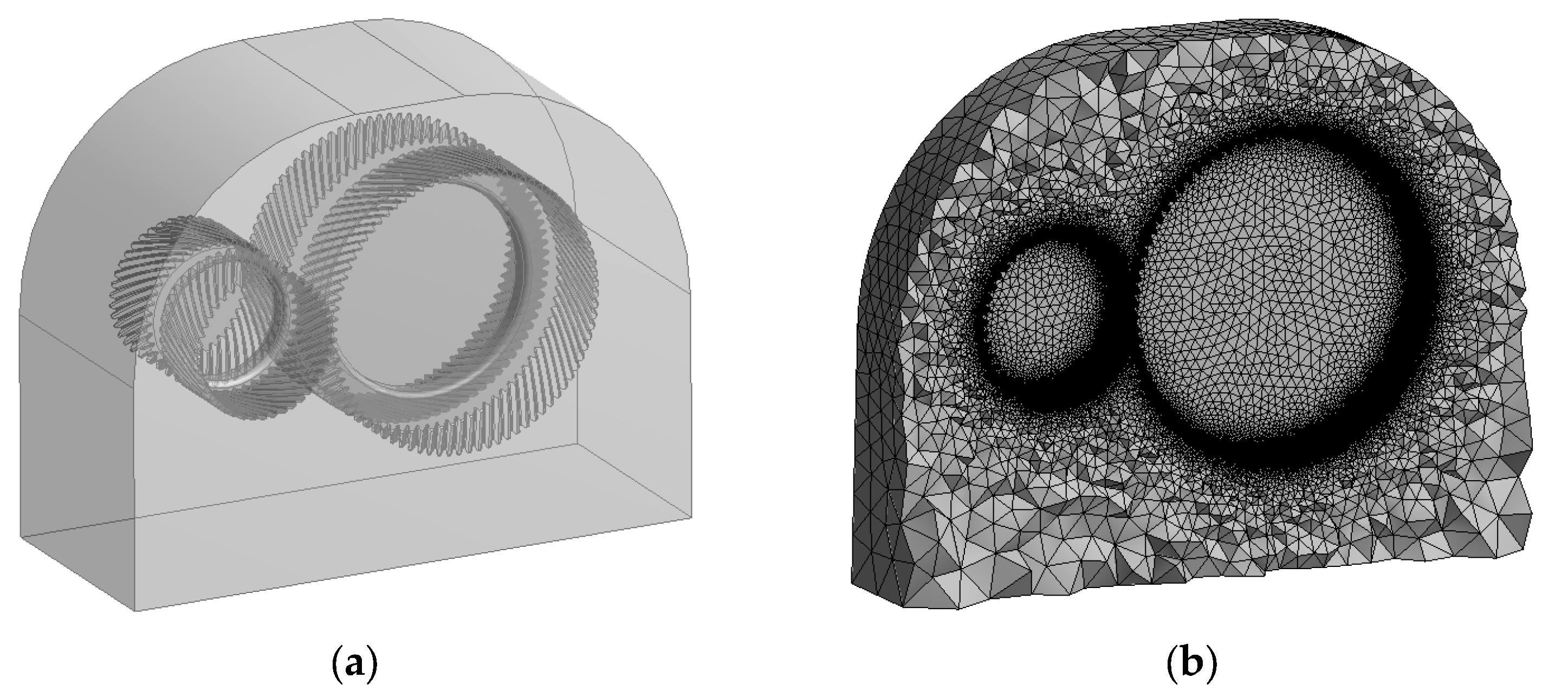
2.2. The CFD Model and the Simulation Settings

After the turbulence model is determined, the simulation analysis model of the high-speed gear transmission system needs to be established. The analysis object is a herringbone gear pair, which adopts a double-gear layout. The basic parameters of the gear are shown in

Table 1. Basic parameters of the gear.

Parameter	Value
Modulus m (mm)	10
Single tooth width B (mm)	260
Pressure angle α (◦)	20
Number of driving gear teeth n1	42
Number of driven gear teeth n2	83
Rated linear speed of the pitch circle v0 (m/s)	150

.

This paper studies the windage characteristics of the gearbox, so it is necessary to analyze the air fluid domain inside the gearbox. The air fluid area in the gearbox is separated, and its three-dimensional model is shown in Figure 1a. Unstructured meshes are used to divide the fluid domain. The meshes are all tetrahedral, with 7,777,897 meshes and 1,471,319 mesh nodes. The mesh division is shown in Figure 1b.

In order to simulate the real movement of the fluid in the gearbox, it is necessary to find a simulation method to simulate the movement of the components. Common simulation methods for moving components are Single Reference Frame, Multiple Reference Frame, Mixing Plane Model, Sliding Mesh Model and Dynamic Mesh. In this study, the Dynamic Mesh model is used. Dynamic Mesh simulates the movement of components by defining the boundary or the movement of mesh nodes, which is the closest simulation technology to the real physical scene.

In the Dynamic Mesh model, the gear is defined as a rotating wall, and the inner wall of the gearbox is defined as a closed wall without slip. Because the meshing clearance of the gear pair is very small, it is easy to report errors of negative volume when using the Dynamic Mesh technology to reconstruct the mesh, so it is necessary to adjust the gear. Common adjustment methods include the two-way tooth cutting method, the modification method, and the separation method, as shown in Figure 2. This paper adopts the separation method to adjust the gear.

When the gear rotates at high speeds, the mesh is distorted, so we need to select smoothing and remeshing in the Dynamic Mesh setting. Smoothing has three methods: spring, diffusion, and linearly elastic solids. In this paper, diffusion is selected. Diffusion is based on solving a diffusion equation to obtain the mesh node displacement:

$$\nabla ·\left(\gamma \nabla u_0\right)=0$$

(6)

where u₀ is the motion speed of the mesh node, and γ is the diffusion coefficient.

Remeshing is used to re-divide unqualified meshes, and needs to be checked by the local face. Then, it is also necessary to set the minimum length scale, maximum length scale, maximum cell skewness and maximum face skewness according to the quality of the mesh.

The rotation of gears in the Dynamic Mesh is usually achieved by writing a profile or user-defined function (UDF) to specify the angular velocity. The profile is simpler than UDF in format, as shown below:

((gear 3 point)

(time t1 t2 t3)

(omega ω₀ ω₀ ω₀))

where, t1, t2, and t3 are three times, and ω₀ is the corresponding angular velocity.

The fluid pressure cannot be directly set in the fluid simulation software. In order to make the pressure inside the gear box a negative pressure, the negative pressure can be realized by changing the air density by referring to the air state equation. The relationship between air pressure and density meets the state equation, which is:

$$p=\rho RT$$

(7)

where p is the pressure, ρ is the fluid density, R is the air constant, and T is the thermodynamic temperature.

In this study, T is set at 300 K, so 0.5 atmospheric pressure can be represented by the state when the air density is 0.588 kg/m³.

The mesh partitioning results are imported into CFD software, and the simulation parameters can be set by referring to

Table 2. The CFD software parameter settings.

Setting	Choice
Solver	Pressure-based
Time	Transient
Viscous model	SST k-ω
Inlet boundary	Velocity-inlet
Outlet boundary	Pressure-outlet
Dynamic mesh	Smoothing and Remeshing
Solution methods	Pressure velocity coupling: SIMPLE Gradient: green-Gauss node based Pressure: PRESTO Momentum: first-order upwind Volume fraction: geo-reconstruct Spatial discretization: first-order upwind
Run calculation	Time step: 2 × 10−6 S Number of time steps: 1250

. A time-step report of the moment of the two gears is set up to record the windage moment of the driving wheel and driven wheel at each time step in the calculation process.

2.3. Windage Moment and Windage Power Loss

The windage moment of the gear consists of a pressure moment and a viscous moment:

$$T_M=T_P+T_V$$

(8)

where T_M is the total windage moment, T_P is the pressure moment, and T_V is the viscous moment.

When the gear rotates at a high speed in the gearbox, the direction of air rotation in the fluid domain is opposite to the direction of gear rotation. At this time, a high-pressure zone is generated on the windward tooth surface of a single tooth due to the air gathering here, while a low-pressure zone is generated on the leeward tooth surface due to the air being taken away, as shown in Figure 3. A vortex also forms in each tooth slot, and the vortex intensifies the flow of air from the leeward tooth surface to the windward tooth surface of the next tooth, to a certain extent. It can be seen from hydromechanics that a local high pressure and a local low pressure produce a pressure difference on the tooth surface and a pressure moment opposite to the rotation direction of the gear [9], which hinders the gear rotation and causes a certain power loss.

Air has a certain viscosity. When air molecules move freely, they suffer a viscous friction force, which is usually called air viscosity or the aerodynamic viscosity coefficient. However, gears rotate in air, so will be hindered by the air viscosity when rotating at high speeds. The viscous moment on the gear is proportional to the contact area, so the viscous moment is generally concentrated on the end face of the gear. The viscous moment on the tooth’s surface is smaller, and the pressure moment is greater on the tooth’s surface.

The windage power loss can be obtained by finite element software simulation or by empirical formula estimation. However, the empirical formula is obtained under standard atmospheric pressure, and cannot directly determine the windage loss under negative pressures in the same way that finite element analysis can.

The windage moment can be obtained through finite element simulation analysis, and then the power loss caused by wind resistance can be obtained according to the conversion formula of power and moment. The conversion formula of power and moment is:

$$P=\frac{T_{0}n}{9550}$$

(9)

where T₀ is the moment, P is the power, and n is the rotational speed.

2.4. Windage Power Loss Prediction

A large number of meshes is used in the fluid simulation analysis, and significant amounts of computer memory and long calculation times are required when using Dynamic Meshes and turbulence models to solve it; this means that the calculation time cost of windage power loss simulation is high. Based on the consideration of time, the existing simulation data and some advanced algorithms are used to predict the windage power loss, which not only saves time costs, but also quickly finds the corresponding windage power loss under different gear speeds and negative pressures. Therefore, a BP neural network optimization algorithm based on a genetic algorithm is selected to predict the windage power loss.

The BP neural network was proposed by Rumelhard and McClelland in 1986 [30]. In terms of structure, it is a typical multilayer feedforward neural network, with one input layer, several hidden layers (either one layer or multiple layers), and one output layer. Layer-to-layer connection is adopted, and there is no interconnection between neurons in the same layer. It has been theoretically proven that a three-layer network with a hidden layer can approximate any nonlinear function. The neurons in the hidden layer mostly use the S-type transfer function, and the neurons in the output layer mostly use the linear transfer function. Figure 4 shows a typical BP neural network structure. The network has a hidden layer. The number of neurons in the input layer is m, the number of neurons in the hidden layer is l, and the number of neurons in the output layer is n. The hidden layer uses an S-type transfer function tan sig, and the transfer function of the output layer is purelin. IW and LW are weights, and b is the bias. The BP neural network uses the back-propagation algorithm to optimize the output. Its basic premise is to learn a certain number of samples; that is, the input of the samples is sent to each neuron of the network input layer. After the calculation of the hidden layer and the output layer, each neuron of the output layer outputs the corresponding predictive value. If the error between the predicted value and the expected output does not meet the accuracy requirements, the error is back-propagated from the output layer to adjust the weight and threshold, so that the error between the network output and the expected output is gradually reduced until the accuracy requirements are met.

Because of the different initial weights and biases, the output results of the BP neural network are different each time. For example, the difference between the predicted results and the actual results once is 4%, and the next time it may reach 10%, which shows a certain instability. In order to solve this instability, the weight and bias of BP neural network are optimized using a genetic algorithm to obtain an optimal weight and bias. The genetic algorithm is an evolutionary algorithm. Its basic principle is to imitate the evolutionary law of “natural selection, survival of the fittest” found in the biological world. The genetic algorithm encodes the problem parameters into chromosomes, and then uses iterative methods for selection, crossover, mutation, and other operations to exchange the information of chromosomes in the population; finally, it generates chromosomes that meet the optimization goal. The BP neural network optimization algorithm based on the genetic algorithm combines the advantages of the genetic algorithm and the neural network; therefore, it can more accurately predict the wind resistance power loss.

3. Results and Analysis

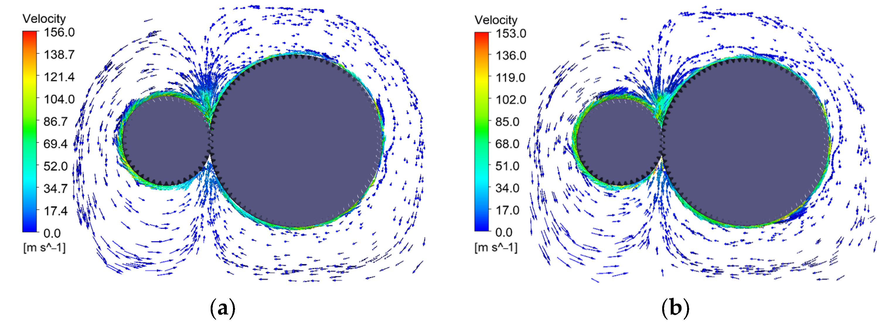
3.1. Flow Field Characteristics and Windage Power Loss under Negative Pressure

When the pressure is 0.5 atm and the speed is 150 m/s, the simulation results are analyzed. In order to better understand the flow state of the fluid inside the gearbox and the mechanism of gear windage power loss, three planes are taken from the fluid domain of the gearbox for analysis. The analysis planes are XY, XZ, and YZ, as shown in Figure 5, where the XY plane is at the center of the gear, the XZ plane is in the gear mesh area, and the YZ plane is in the middle of a single gear.

The YZ plane reflects the overall flow state of the air inside the gearbox, and its pressure cloud diagram is shown in Figure 6. The figure shows that the pressure at the inlet side of the meshing area is positive, and the pressure at the outlet side of the meshing area is negative. At this time, the air at the inlet side of the meshing area converges here due to the rotation of the gear, resulting in a gradual increase in the pressure here; the maximum is 1.2 × 10⁴ Pa. The gear at the outlet side of the meshing area is disengaged, which makes the space volume larger, thus generating negative pressure; the minimum is −4.6 × 10⁴ Pa. Taking the gear pitch point as the origin of the Z coordinate, the change curve of pressure with the Z coordinate can be obtained, as shown in Figure 7. It can be seen that the pressure changes significantly near the meshing area, indicating that the flow field in the meshing area is violent.

Figure 8 shows the velocity distribution cloud diagram of the fluid in the high-speed gearbox on the YZ plane. The figure shows that the closer the gear surface is, the higher the fluid flow velocity will be, indicating that the gear surface is the key area for windage power loss. It can be seen from observing the speed that the speed near the gear pitch point can exceed the gear rotation speed, and the maximum speed is 219.6 m/s. The rapid change in pressure causes a change in the fluid flow velocity, so there will be obvious velocity-decreasing areas at the inlet side and outlet side of the meshing area, and the velocity-decreasing area at the outlet side is larger than that at the inlet side.

The velocity vector diagram of the YZ plane flow field is shown in Figure 9, and its maximum velocity vector is 154.9 m/s. It can be seen from Figure 9 that the speed direction of the fluid near the tooth surface is consistent with the direction of the gear rotation, while the speed direction of the fluid away from the tooth surface is opposite to the direction of the gear rotation. This flow change can be explained by the pressure cloud diagram in Figure 6: the air in the fluid domain flows from the high-pressure area at the inlet side of the meshing area to the low-pressure area at the outlet side, forming a flow opposite to the rotation direction of the gear. The airflow direction near the tooth surface is not consistent with that observed far away from the tooth surface, which leads to a vortex near the interface of the two kinds of airflow, and this vortex will cause a certain fluid eddy loss.

The XZ and XY planes reflect the flow of fluid in the meshing area and tooth surface. Figure 10 shows the pressure cloud map of gearbox fluid in the XZ and XY planes. The figure shows that the pressure changes obviously near the gear meshing area, indicating that the fluid flow in these areas is intense. In Figure 10a, the pressure at the inlet side of the meshing area decreases outward from the meshing center along the direction of the gear helix angle; for example, the pressure at the left of the inlet side of the meshing area decreases along the upper left, as shown by the arrow in Figure 10a. The pressure change in the outlet side of the meshing area is not obvious as that on the inlet side, but it can also be seen that the pressure changes along the direction of the gear helix angle. In Figure 10b, there is a large negative pressure at the middle meshing clearance of the gear, while the pressure change in other places is not obvious. Small orange high-pressure areas can be found on both walls along the axial direction of the meshing.

The fluid velocity distribution in the XZ and XY planes is shown in Figure 11. It can be seen that the fluid velocity near the gear is very high, and the fast-flowing air is the main reason for the windage loss. Figure 11a shows the velocity of fluid in the XZ plane. The figure shows that the velocity change near the meshing area is most obvious, and the velocity decreases outward from the meshing center. In Figure 11b, the air speed near the gear tooth surface is high, while the speed in other areas is relatively low.

The velocity vector distribution in the XZ plane is shown in Figure 12a. Four clear vortices can be seen near the gear mesh, which cause fluid eddy current loss. The direction of vortex rotation can be explained by the pressure distribution seen in Figure 10a: the pressure on the left side of the inlet side of the meshing area decreases along the upper left side, so the direction of vortex rotation on the left side is clockwise. Similarly, the right side rotates counterclockwise. The pressure on the left side of the outlet side of the meshing area also decreases along the upper left side, but the negative pressure generates suction, so the fluid rotates counterclockwise; similarly, the right side rotates clockwise. The pressure at the middle groove of the XZ plane is lower than that around it, causing the fluid to flow to the middle groove of the gear. In this way, the intersection of the upper and lower airflow at the outlet side of the meshing area generates a local high pressure, forcing the intersection airflow to flow to the left and right sides, which further strengthens the strength of the two vortices below the gear, so there are more velocity vector lines at the outlet side of the meshing area.

The velocity vector distribution in the XY plane is shown in Figure 12b. A vortex with the same rotation direction as that in the XZ plane can be seen above the driven gear and below the driving gear. Figure 10b shows that there is a small high-pressure area on both sides of the meshing position, and the pressure on the upper and lower parts of the meshing position side is low, which causes the velocity vector on the side of the two gears in Figure 12b to flow away from the meshing position.

Comparing the pressure distribution of the XZ plane under negative pressure with that observed under ordinary pressures, we obtain Figure 13. This figure shows that the pressure distribution at 0.5 atm is similar to that at ordinary pressures. However, the pressure value changed significantly. The maximum pressure decreased from 2.0 × 10⁴ Pa to 1.3 × 10⁴ Pa, a decrease of 35%, and the minimum pressure also decreased by 50.4%. The comparison of velocity vector distribution in the YZ plane is shown in Figure 14. It can be seen that the flow direction of air is the same under negative pressure and ordinary pressure, but the maximum velocity value is reduced by 2%. Therefore, from the finite element simulation results, the negative pressure environment can be seen to have a relatively small impact on the distribution of the characteristics of the air-flow field in the gearbox, but it has a greater impact on the numerical value.

The total moment received by the driven wheel at 0.5 atm is taken as an example. At the beginning of rotation, a large windage moment (about 1700 N·m) is generated, and then the moment rapidly declines and gradually becomes stable, as shown in Figure 15. In this paper, the stabilized moment is taken as the analysis data.

Referring to the relevant papers [4], it can be seen that windage moment values of the driving wheel and the driven wheel of the gear are different, and the proportion of pressure moment and viscous moment is also different. The windage moment data under negative pressures can be obtained by taking the simulation data results of the last time step, as shown in

Table 3. Windage moment distribution of the gear at 0.5 atm.

	Pressure Moment of Driven Gear (N·m)	Viscous Moment of Driven Gear (N·m)	Pressure Moment of Driving Gear (N·m)	Viscous Moment of Driving Gear (N·m)
Value	−216.42	−16.50	70.82	3.47

.

Table 3 shows that the windage moment of the gear under negative pressure is mainly the pressure moment, indicating that the windage moment is mainly generated by the tooth surface rather than the gear end-face. The proportion of the two kinds of moment to the total moment is drawn, as shown in Figure 16. The viscous moment accounts for more in the driven wheel, up to 7.08%, and less in the driving wheel.

Comparing the moment at 0.5 atm with that at ordinary pressure,

Table 4. Comparison of windage moment distribution.

	Pressure Moment of Driven Gear (N·m)	Viscous Moment of Driven Gear(N·m)	Pressure Moment of Driving Gear(N·m)	Viscous Moment of Driving Gear (N·m)	Total Moment (N·m)
1 atm	−437.51	−28.41	140.07	6.06	612.05
0.5 atm	−216.42	−16.50	70.82	3.47	307.21

can be obtained. The table shows that the total windage moment under negative pressure is 49.8% less than that under ordinary pressure. Comparing the proportion of the two kinds of moments to the total moment with that at ordinary pressure, Figure 17 can be obtained. Figure 17 shows that the pressure moment always accounts for more than 92% of the total moment, and the proportion of the pressure moment under negative pressure decreases compared with that at ordinary pressure, while the proportion of viscous moment increases.

Figure 15 shows that the windage moment tends to be gentle after the flow field is stabilized, but there are still slight moment fluctuations. In order to obtain more reliable values, the average value of the moment in the last 50 time steps is taken as the gear moment obtained by fluid simulation. After average treatment, the windage moment of the driven wheel is 231.81 N·m and that of the driving wheel is 74.53 N·m at 0.5 atm, so the windage power loss of the driven wheel is 74.0 kW and that of the driving wheel is 47.0 kW. At this time, the total windage power loss of the gear is 121.0 kW.

In order to understand the influence of negative pressure on windage power loss, the windage power loss under negative pressure is compared with that under ordinary pressure, as shown in

Table 5. Comparison of windage power loss.

	Driven Gear Moment (N·m)	Driving Gear Moment (N·m)	Driven Gear Windage Loss (kW)	Driving Gear Windage Loss (kW)	Total Windage Loss (kW)
1 atm	−462.56	147.55	147.6	93.1	240.7
0.5 atm	−231.81	74.53	74.0	47.0	121.0

. Table 5 shows that the total power lost by gear rotation at 0.5 atmospheric pressure is 49.7% less than that at ordinary pressure. Therefore, it can be seen that the windage power loss under negative pressure is lower; that is, reducing the pressure in the gear box can effectively reduce the windage power loss caused by the windage moment.

3.2. Effect of Different Parameters on Windage Power Loss

When the speed is high, each tooth surface will produce a large windage moment and hinder the rotation of the gear, resulting in windage power loss, which reduces the transmission efficiency of the gearbox. In order to improve the transmission efficiency of high-speed gearbox and reduce the windage power loss, it is necessary to analyze the effect of gear speed on the windage power loss of the gearbox. In addition to the gear speed, it can be seen from the previous analysis that different pressures in the gearbox also affect the size of the windage moment. It is also necessary to study the windage power loss of the gearbox under different negative pressure environments. This paper analyzes the windage power loss at different speeds under the same pressure and at different negative pressures under the same speed.

First, when the pressure in the gearbox is constant, the effect of different gear speeds on the windage power loss can be analyzed. The average value of the windage moment at 0.9 atmospheric pressure and different speeds was obtained, and then the corresponding windage power loss was obtained through the conversion formula of moment and power.

Table 6. Windage power loss at 0.9 atm.

Speed (m/s)	Windage Power Loss (kW)
120	110.14
130	141.39
140	176.22
150	216.92
160	264.23
170	317.04

and Figure 18 were obtained after sorting. Figure 18 shows that, when the speed increases by 10 units at 0.9 atmospheric pressure, the windage power loss increases accordingly more. The windage power loss increases exponentially with the increase in the gear linear speed, which is consistent with the data in the relevant papers [31,32,33,34]. Therefore, on the basis of ensuring the transmission efficiency, the speed of the gear should not be too high, as this can easily produce greater windage power loss [27].

By further analyzing the windage power loss data at 0.3 atmospheric pressure and comparing the obtained data with those at 0.9 atmospheric pressure, Figure 19 can be obtained. Figure 19 shows that the windage power loss increases exponentially with the increase in speed at 0.3 atmospheric pressure, but the windage power loss growth rate at 0.3 atm is lower than that at 0.9 atm, and the windage loss at 0.3 atm is smaller than that at 0.9 atm under the same speed.

Then, we further studied the effect of gearbox pressure on windage power loss when the speed of gear is constant. The pressure in the gearbox is equidistant from 0.2 to 1 atmosphere, and the simulation analysis is conducted at a speed of 120 m/s.

Table 7. Windage power loss at 120 m/s.

Pressure (atm)	Windage Power Loss (kW)
0.2	24.9
0.3	38.9
0.4	49.1
0.5	63.0
0.6	74.3
0.7	85.4
0.8	98.0
0.9	110.1
1	122.2

was obtained by sorting out the gathered data. Table 7 shows that the windage power loss varies linearly with the increase in gearbox pressure, indicating that the smaller the pressure is, the smaller the windage power loss of the gear is.

When 150 m/s and 170 m/s are added, the variation rule of windage power loss with gearbox pressure can be seen in Figure 20. Figure 20 shows that the windage power loss varies linearly with the increase in gearbox pressure at three different speeds, but the slopes of the three curves are different. The higher the speed, the greater the slope of the curve. It can be seen from the figure that the greater the speed and pressure, the greater the windage power loss caused by air. Therefore, on the basis of manufacturing costs, lower pressures should be selected to effectively reduce the windage power loss of the gearbox and improve the transmission efficiency of the gear transmission system.

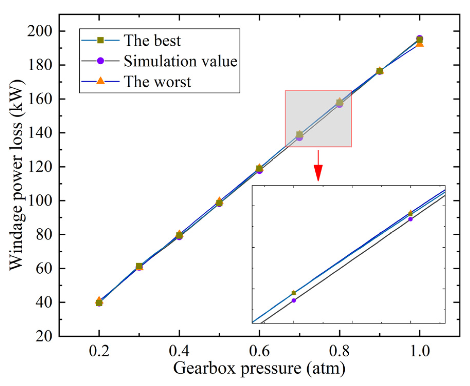
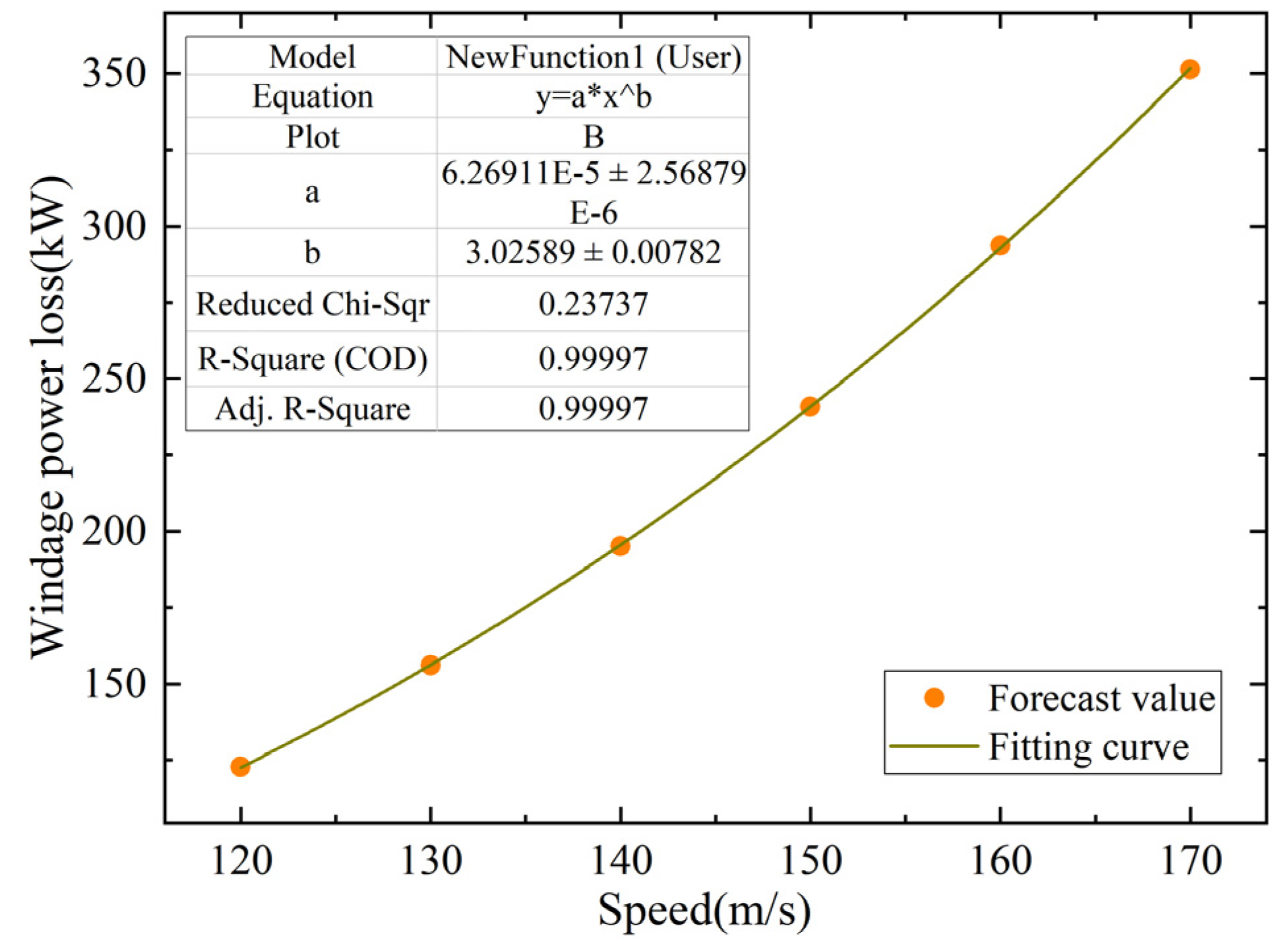
3.3. Windage Power Loss Prediction

We took the data of windage loss changes with gearbox pressure at 120 m/s, 150 m/s and 170 m/s, and the data of windage loss changes with speed at 0.3 atm. The four groups of original data were used to predict the change rule of windage power loss with gearbox pressure when the speed is 140 m/s. Meanwhile, numerical simulation is carried out for the model with the speed of 140m/s, and its numerical simulation data is obtained. The error of the prediction data and simulation data were compared to assess the reliability of prediction data. In order to ensure the reliability of data, BP neural network based on genetic algorithm is used to predict for five times, and the best data and the worst data are compared with the numerical simulation data obtained using the finite element method. The prediction results are shown in

Table 8. Predicted windage power loss at 140 m/s.

Pressure (atm)	Simulation Value (kW)	The Worst of Five Times	The Best of Five Times
0.2	39.64	43.90 (10.7%)	39.08 (1.4%)
0.3	60.62	60.58 (0.06%)	60.63 (0.02%)
0.4	78.79	73.04 (7.3%)	79.13 (0.4%)
0.5	98.28	88.29 (10.2%)	98.91 (0.6%)
0.6	117.84	107.14 (9.1%)	120.03 (1.9%)
0.7	137.19	131.04 (4.5%)	141.31 (3.0%)
0.8	156.71	151.50 (3.3%)	162.28 (3.6%)
0.9	176.22	167.74 (4.8%)	182.82 (3.8%)
1	195.53	185.56 (5.1%)	202.76 (3.7%)

below. The data in the third and fourth columns are the predicted values, and the percentage in the brackets is the error between the predicted values and the simulated values. Table 8 shows that, on the basis of four sets of original data, the maximum prediction error of the worst group is 10.7%, the maximum prediction error of the best group is 3.8%, and the maximum data difference is within 10 kW. Data comparison (Figure 21) shows that there is an obvious error between the worst group and the simulation value, and the best group is close to the simulation value.

Then, the windage power loss data were added at different speeds at 0.9 atmospheric pressure. At this time, there are five groups of original data. After sorting out the windage power loss prediction results at different pressures at 140 m/s, we obtain

Table 9. Predicted windage power loss at 140 m/s (increase in a group of data).

Pressure (atm)	Simulation Value (kW)	The Worst of Five Times	The Best of Five Times
0.2	39.64	40.80 (2.9%)	39.57 (0.2%)
0.3	60.62	60.48 (0.2%)	61.38 (1.3%)
0.4	78.79	80.11 (1.7%)	79.28 (0.6%)
0.5	98.28	99.63 (1.4%)	98.48 (0.2%)
0.6	117.84	119.25 (1.2%)	118.94 (1.0%)
0.7	137.19	138.99 (1.3%)	138.94 (1.3%)
0.8	156.71	158.34 (1.0%)	157.88 (0.7%)
0.9	176.22	176.39 (0.1%)	176.24 (0.02%)
1	195.53	192.29 (1.7%)	195.02 (0.3%)

. The table shows that the maximum prediction error of the worst group is 2.9%, and the maximum prediction error of the best group is 1.3%. The error is much smaller, and the maximum difference is also reduced from 10 kW to within 4 kW. By observing the comparison between the predicted data and the simulated data in Figure 22, it is found that both the best group and the worst group are very close to the simulated value, indicating the high accuracy of the prediction. Therefore, within a certain allowable range of error, the predicted data can be considered to be reasonable and can be used to estimate the simulation value.

Using the above model with five groups of original data to predict the windage power loss at different speeds under ordinary pressure (1 atm),

Table 10. Predicted windage loss under ordinary pressure.

Speed (m/s)	Predicted Windage Loss (kW)
120	122.8
130	156.1
140	195.1
150	240.9
160	293.6
170	351.4

can be obtained. By curve fitting the data in Table 10, the relationship between windage power loss P and speed v₀ can be obtained; that is, P = 6.26911 × 10⁻⁵ × v₀^3.02589, as shown in Figure 23. It can be seen that P has a linear relationship with v₀^3.02589, which is in good agreement with the data in the open literature [3,9,10,11,15,32,33,34], verifying the accuracy of the prediction model.

4. Conclusions

This paper studies the windage characteristics of a high-speed gearbox based on negative pressure regulation. First, for the double herringbone gear transmission system, based on the CFD theory, a simulation analysis model of high-speed gear windage characteristics under ordinary pressure and negative pressure is established. Then, the flow field characteristics and windage power loss of a high-speed gear pair under negative pressure are analyzed in detail, and are then compared with the ordinary pressure. On this basis, the effects of different gear speed and different gearbox pressures on the windage loss is further explored. Finally, the windage power loss of high-speed gears is predicted numerically by using neural networks. Based on the research and analysis in this paper, the following conclusions can be drawn:

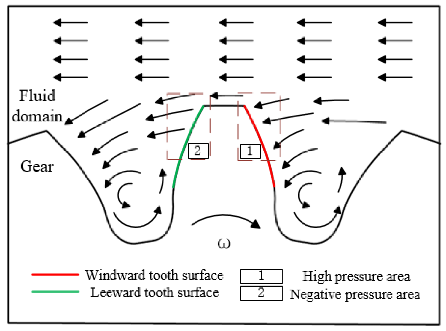
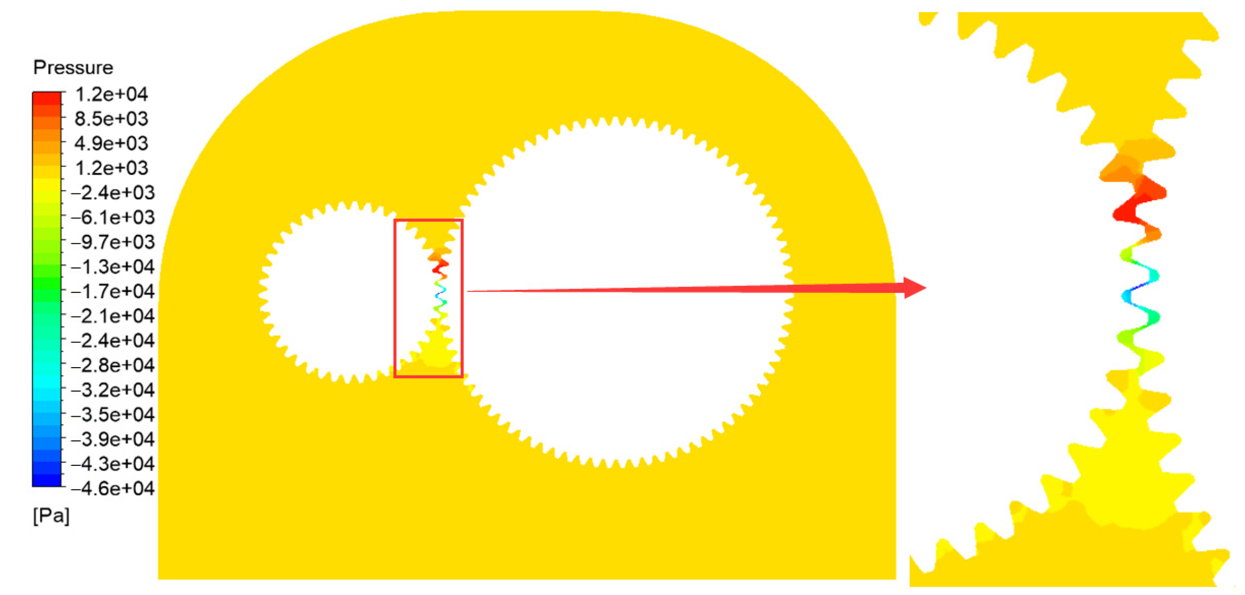
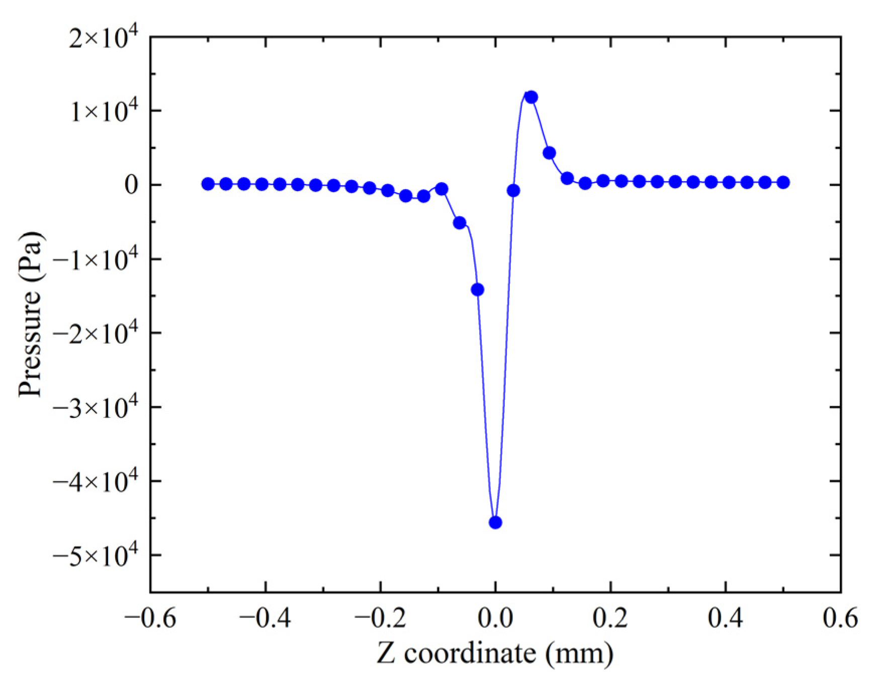
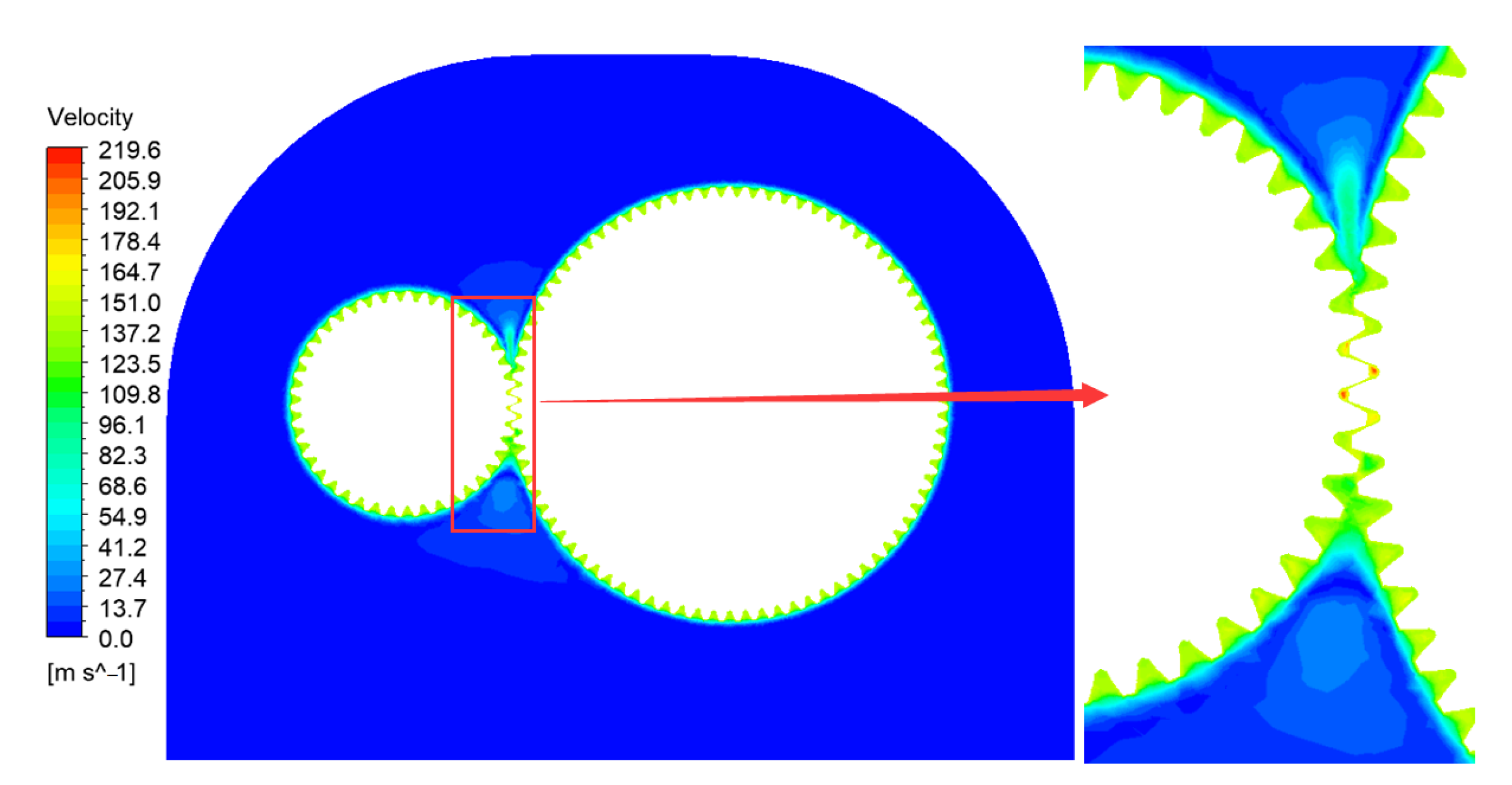
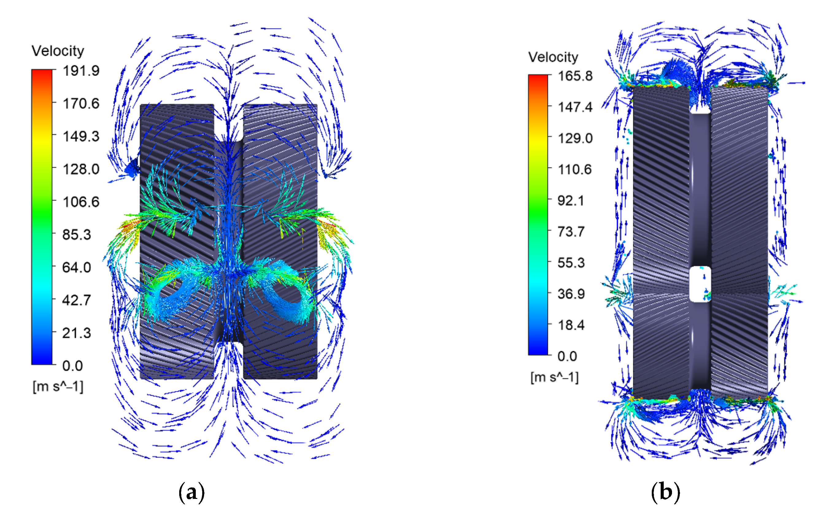
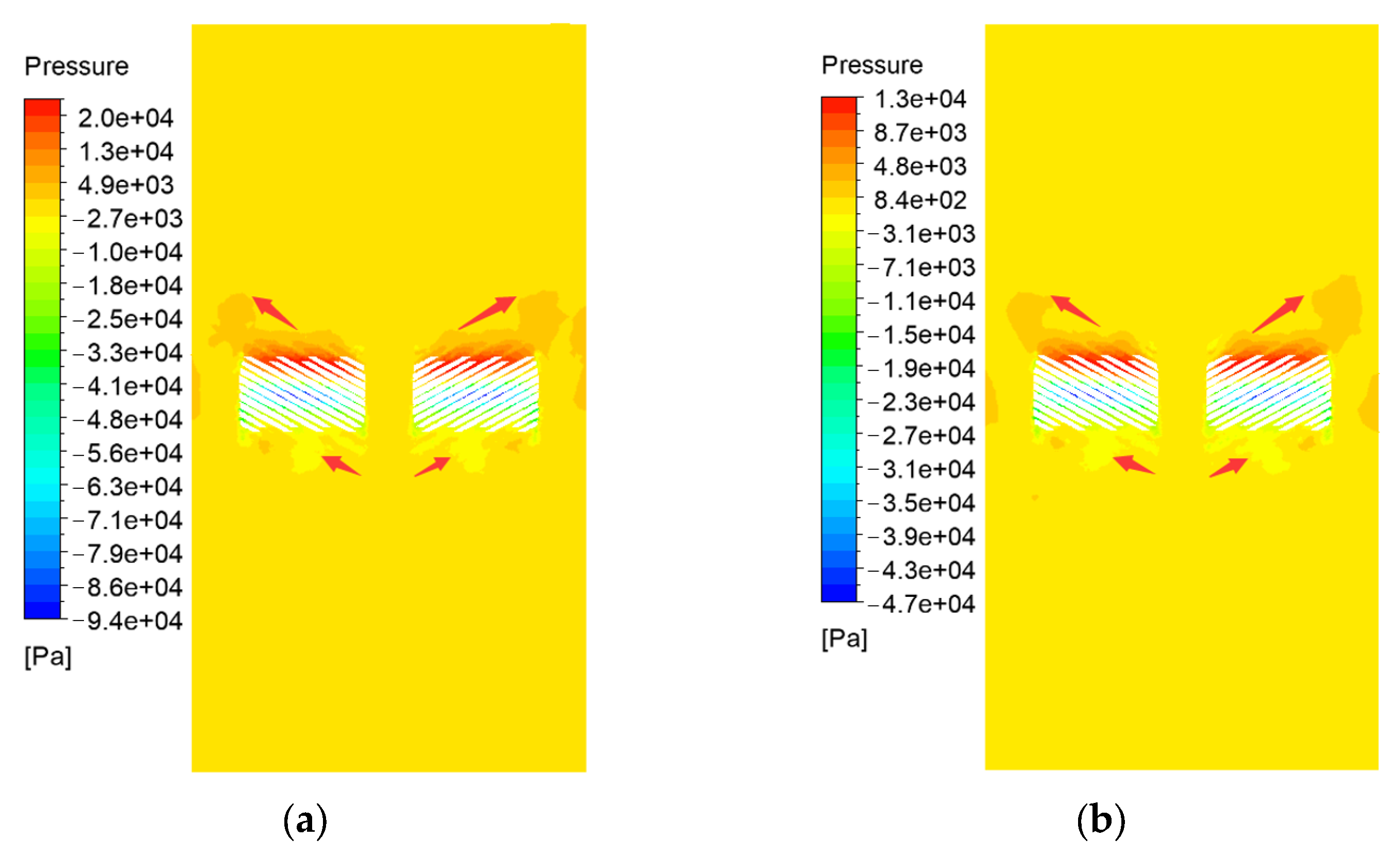
• The airflow in the meshing area of the gearbox is violent, which easily generates vortices. The air flowing at high speeds near the tooth surface produces a large pressure moment, which is the main reason for the windage loss. Under negative pressures, the airflow direction near the gear tooth surface is opposite to that observed far away from the tooth surface, which provides strong evidence for the generation of vortices in the gearbox.
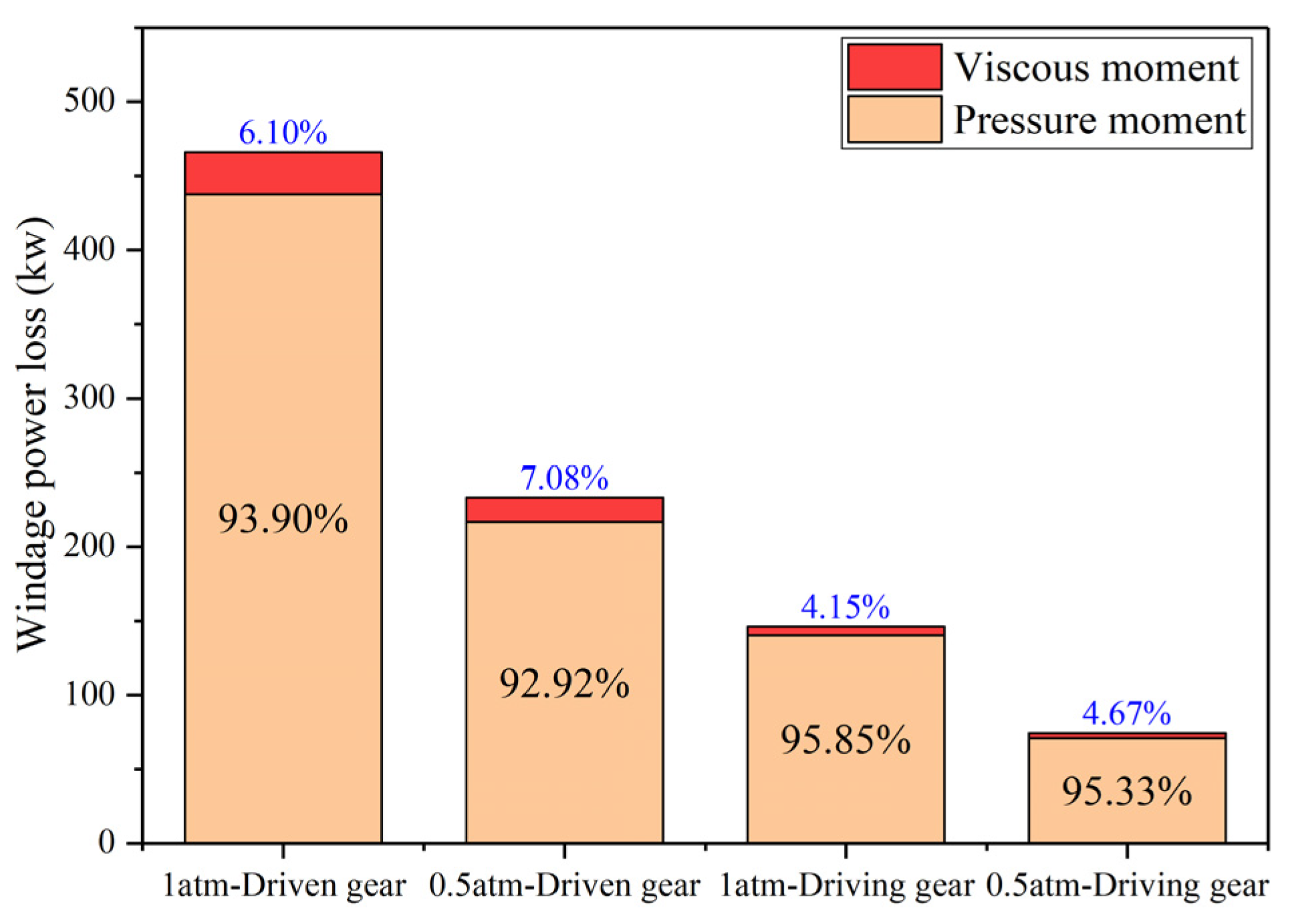
• The flow field characteristics of the high-speed gearbox at 0.5 atm are basically the same as those at ordinary pressures, but the windage moment at 0.5 atm is reduced by 49.8% and the windage loss is reduced by 49.7% compared with the values obtained at ordinary pressures.
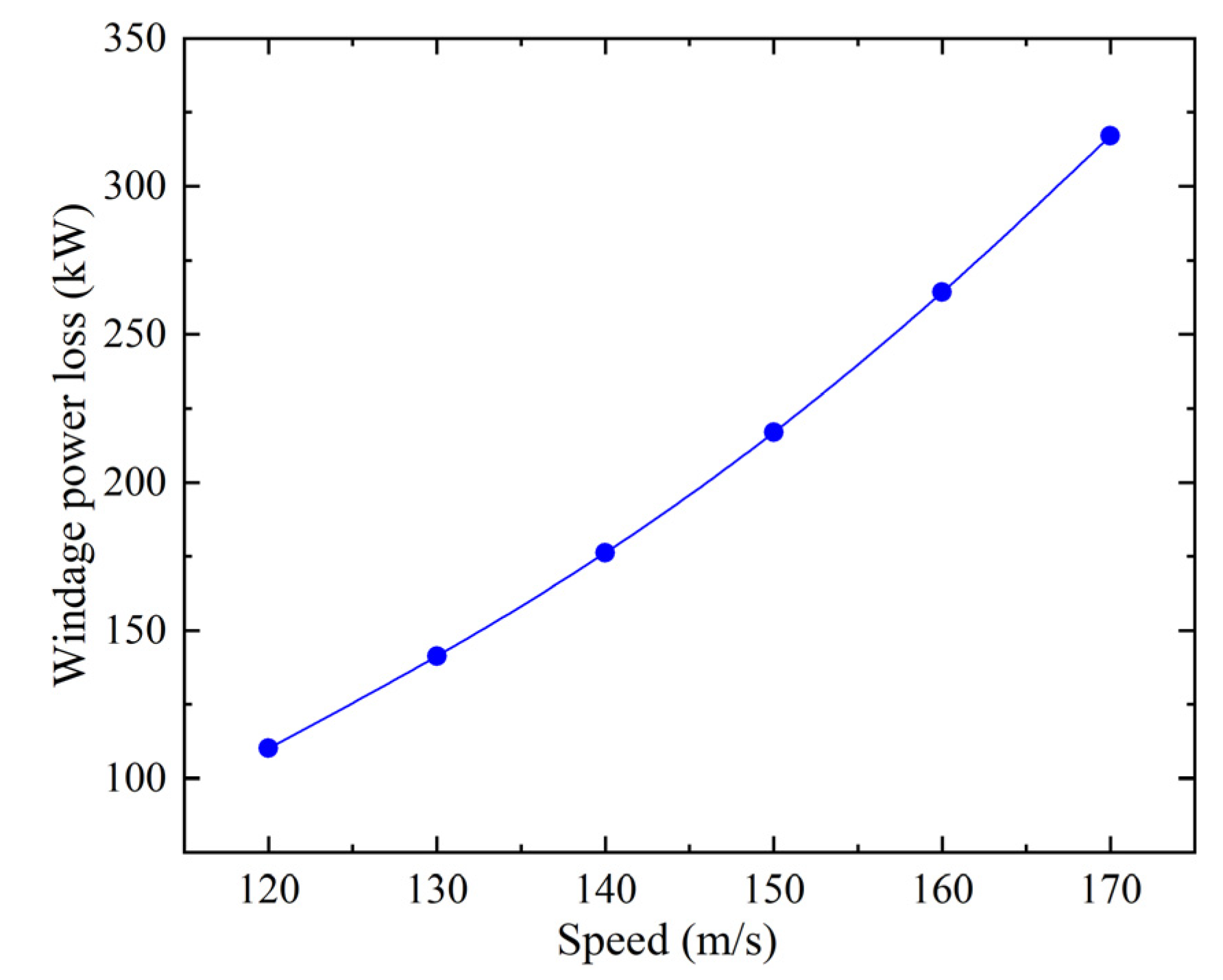
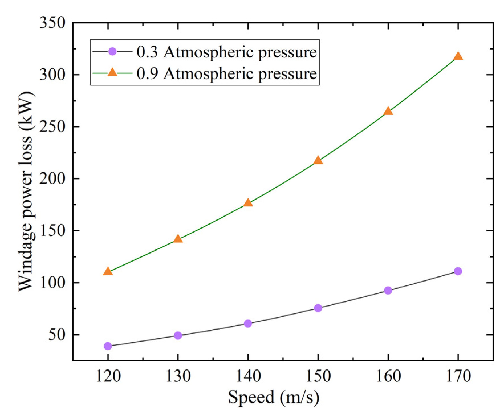
• The windage power loss increases linearly with the increase in gearbox pressure and exponentially with the increase in speed. Therefore, the windage power loss is minimum at lower gearbox pressures and gear speeds.
• The prediction results of the BP neural network optimization algorithm based on the genetic algorithm are in good agreement with the finite element simulation data and the open literature, showing that it has high prediction accuracy and can effectively save simulation analysis time.

Although this study shows that a negative pressure environment can reduce the windage power loss, there is still a lack of research on gear oil-spraying lubrication under negative pressures, as well as a lack of certain experimental verification. In the future, experiments involving high-speed gearboxes under negative pressure will be carried out to verify the consistency of the experimental results and simulation data, so as to break through the transmission efficiency improvement technology of high-speed gearbox based on negative pressure regulation.

References

1. Zhu, X.; Dai, Y.; Ma, F. CFD modelling and numerical simulation on windage power loss of aeronautic high-speed spiral bevel gears. Simul. Model. Pract. Theory 2020, 103, 102080. [Google Scholar] [CrossRef]
2. Dai, Y.; Ma, F.; Zhu, X.; Jia, J. Numerical simulation investigation on the windage power loss of a high-speed face gear drive. Energies 2019, 12, 2093. [Google Scholar] [CrossRef] [Green Version]
3. Fondelli, T.; Andreini, A.; Facchini, B. Numerical investigation on windage losses of high-speed gears in enclosed configuration. AIAA J. 2018, 56, 1910–1921. [Google Scholar] [CrossRef]
4. Zhang, Y.; Hou, X.; Zhang, H.; Zhao, J. Numerical simulation on windage power loss of high-speed spur gear with baffles. Machines 2022, 10, 416. [Google Scholar] [CrossRef]
5. Concli, F.; Gorla, C. Analysis of the power losses in geared transmissions–measurements and CFD calculations based on open source codes. In Proceedings of the Open Source CFD International Conference 2013, Hamburg, Germany, 24–25 October 2013. [Google Scholar]
6. Zhu, X.; Dai, Y.; Ma, F. Development of a quasi-analytical model to predict the windage power losses of a spiral bevel gear. Tribol. Int. 2020, 146, 106258. [Google Scholar] [CrossRef]
7. Massini, D.; Fondelli, T.; Andreini, A.; Facchini, B.; Tarchi, L.; Leonardi, F. Experimental and numerical investigation on windage power losses in high speed gears. In Proceedings of the ASME Turbo Expo 2017, Charlotte, NC, USA, 26–30 June 2017. [Google Scholar]
8. Handschuh, R.R.; Kilmain, C.J. Efficiency of High-Speed Helical Gear Trains; Technical Report NASA/TM-2003-212222; ARL-TR-2968; Cleveland OH Glenn Research Center: Cleveland, OH, USA, 2003. [Google Scholar]
9. Li, L.; Wang, S.; Zou, H.; Cao, P. Windage loss characteristics of aviation spiral bevel gear and windage reduction mechanism of shroud. Machines 2022, 10, 390. [Google Scholar] [CrossRef]
10. Bianchini, C.; Da Soghe, R.; Errico, J.D.; Tarchi, L. Computational analysis of windage losses in an epicyclic gear train. In Proceedings of the ASME Turbo Expo 2017, Charlotte, NC, USA, 26–30 June 2017. [Google Scholar]
11. Diab, Y.; Ville, F.; Velex, P.; Changenet, C. Windage losses in high speed gears—Preliminary experimental and theoretical results. J. Mech. Des. 2004, 126, 903–908. [Google Scholar] [CrossRef]
12. Aktas, M.K.; Yavuz, M.A.; Ersan, A.K. Computational fluid dynamics simulations of windage loss in a spur gear. In Proceedings of the ASME Turbo Expo 2018, Oslo, Norway, 11–15 June 2018. [Google Scholar]
13. Rapley, S.; Eastwick, C.; Simmons, K. The application of CFD to model windage power loss from a spiral bevel gear. In Proceedings of the ASME Turbo Expo 2007, Montreal, QC, Canada, 14–17 May 2007. [Google Scholar]
14. Rapley, S.; Eastwick, C.; Simmons, K. Effect of variations in shroud geometry on single phase flow over a shrouded single spiral gear. In Proceedings of the ASME Turbo Expo 2008, Berlin, Germany, 9–13 June 2008. [Google Scholar]
15. Arisawa, H.; Nishimura, M.; Imai, H.; Goi, T. CFD simulation for reduction of oil churning loss and windage loss on aeroengine transmission gears. In Proceedings of the ASME Turbo Expo 2009, Orlando, FL, USA, 8–12 June 2009. [Google Scholar]
16. He, A.; Deng, R.; Xiong, Y. CFD study on the windage power loss of high speed gear. In Proceedings of the 2018 5th International Conference on Advanced Materials, Mechanics and Structural Engineering, Seoul, Republic of Korea, 19–21 October 2018. [Google Scholar]
17. Hill, M.J.; Kunz, R.F.; Medvitz, R.B.; Handschuh, R.F.; Long, L.N.; Noack, R.W.; Morris, P.J. CFD analysis of gear windage losses: Validation and parametric aerodynamic studies. J. Fluid. Eng. 2011, 133, 031103. [Google Scholar] [CrossRef] [Green Version]
18. Li, S.; Li, L. Computational investigation of baffle influence on windage loss in helical geared transmissions. Tribol. Int. 2021, 156, 106852. [Google Scholar] [CrossRef]
19. Al-Shibl, K.; Simmons, K.; Eastwick, C. Modelling windage power loss from an enclosed spur gear. Proc. Inst. Mech. Eng. Part A J. Power Energy 2007, 221, 331–341. [Google Scholar] [CrossRef] [Green Version]
20. Zhao, N.; Jia, Q.J. Research on windage power loss of spur gear base on CFD. Appl. Mech. Mater. 2012, 184, 450–455. [Google Scholar] [CrossRef]
21. Zhang, Y.; Li, L.; Zhao, Z. Optimal design of computational fluid dynamics: Numerical calculation and simulation analysis of windage power losses in the aviation. Processes 2021, 9, 1999. [Google Scholar] [CrossRef]
22. Yang, Y.; Zhang, H.; Hong, Z. Research on optimal design method for drag reduction of vacuum pipeline vehicle body. Int. J. Comput. Fluid. D 2019, 33, 77–86. [Google Scholar] [CrossRef]
23. Gillani, S.; Panikulam, V.; Sadasivan, S.; Yaoping, Z. CFD analysis of aerodynamic drag effects on vacuum tube trains. J. Appl. Fluid Mech. 2019, 12, 303–309. [Google Scholar] [CrossRef]
24. Zhang, Y. Numerical simulation and analysis of aerodynamic drag on a subsonic train in evacuated tube transportation. J. Mod. Transp. 2012, 20, 44–48. [Google Scholar] [CrossRef] [Green Version]
25. Chen, X.; Zhao, L.; Ma, J.; Liu, Y. Aerodynamic simulation of evacuated tube maglev trains with different streamlined designs. J. Mod. Transp. 2012, 20, 115–120. [Google Scholar] [CrossRef] [Green Version]
26. Oh, J.-S.; Kang, T.; Ham, S.; Lee, K.-S.; Jang, Y.-J.; Ryou, H.-S.; Ryu, J. Numerical analysis of aerodynamic characteristics of hyperloop system. Energies 2019, 12, 518. [Google Scholar] [CrossRef] [Green Version]
27. Zhu, X.; Dai, Y.; Ma, F. On the estimation of the windage power losses of spiral bevel gears: An analytical model and CFD investigation. Simul. Model. Pract. Theory 2021, 110, 102334. [Google Scholar] [CrossRef]
28. Li, J.; Qian, X.; Liu, C. Comparative study of different moving mesh strategies for investigating oil flow inside a gearbox. Int. J. Numer Method H 2022, 32, 3504–3525. [Google Scholar] [CrossRef]
29. Menter, F. Zonal two equation k-w turbulence models for aerodynamic flows. In Proceedings of the 23rd Fluid Dynamics, Plasmadynamics, and Lasers Conference, Orlando, FL, USA, 6–9 July 1993. [Google Scholar]
30. Wang, P.; Zhu, L.; Zhu, Q.; Ji, X.; Wang, H.; Tian, G.; Yao, E. An application of back propagation neural network for the steel stress detection based on barkhausen noise theory. Ndt E Int. 2013, 55, 9–14. [Google Scholar] [CrossRef]
31. Gorla, C.; Concli, F.; Stahl, K.; Hhn, B.; Michaelis, K.; Schulthei, H.; Stemplinger, J. Hydraulic losses of a gearbox: CFD analysis and experiments. Tribol. Int. 2013, 66, 337–344. [Google Scholar] [CrossRef]
32. Dudley, D.W. Dudley’s Gear Handbook: The Design, Manufacture, and Application of Gears; McGraw Hill Higher Education: Irvine, CA, USA, 1962; pp. 14–21. [Google Scholar]
33. Eastwick, C.N.; Johnson, G. Gear windage: A review. J. Mech. Design. 2008, 130, 034001. [Google Scholar] [CrossRef]
34. Handschuh, R.F.; Kilmain, C.J. Preliminary comparison of experimental and analytical efficiency results of high-speed helical gear trains. In Proceedings of the ASME 2003 International Design Engineering Technical Conferences and Computers and Information in Engineering Conference, Chicago, IL, USA, 2–6 September 2003. [Google Scholar]
Figure 1. Fluid domain setting: (a) three-dimensional model; (b) mesh division.
Processes 11 00804 g001
Figure 2. Adjustment methods: (a) ywo-way tooth cutting method; (b) modification method; (c) separation method.
Processes 11 00804 g002
Figure 3. Demonstration diagram of pressure moment formation.
Processes 11 00804 g003
Figure 4. BP neural network structure diagram.
Processes 11 00804 g004
Figure 5. The plane division diagram.
Processes 11 00804 g005
Figure 6. YZ plane pressure cloud map.
Processes 11 00804 g006
Figure 7. Pressure variation with Z coordinate.
Processes 11 00804 g007
Figure 8. YZ plane velocity cloud map.
Processes 11 00804 g008
Figure 9. Velocity vector of the YZ plane.
Processes 11 00804 g009
Figure 10. Plane pressure cloud map: (a) XZ plane; (b) XY plane.
Processes 11 00804 g010
Figure 11. Plane speed cloud map: (a) XZ plane; (b) XY plane.
Processes 11 00804 g011
Figure 12. Plane velocity vector diagram: (a) XZ plane; (b) XY plane.
Processes 11 00804 g012
Figure 13. Comparison of the XZ plane pressure cloud map: (a) ordinary pressure; (b) 0.5 atm.
Processes 11 00804 g013
Figure 14. Comparison of the YZ plane velocity vector: (a) ordinary pressure; (b) 0.5 atm.
Processes 11 00804 g014
Figure 15. Moment versus time.
Processes 11 00804 g015
Figure 16. Percentage of two moments at 0.5 atm.
Processes 11 00804 g016
Figure 17. Comparison of percentage of windage loss.
Processes 11 00804 g017
Figure 18. Effect of speed on windage power loss at 0.9 atm.
Processes 11 00804 g018
Figure 19. Effect of speed on windage power loss at 0.3 and 0.9 atm.
Processes 11 00804 g019
Figure 20. Effect of pressure on windage power loss at 120 m/s, 150 m/s, and 170 m/s.
Processes 11 00804 g020
Figure 21. Data comparison diagram.
Processes 11 00804 g021
Figure 22. Data comparison diagram (increase in a group of data).
Processes 11 00804 g022
Figure 23. Prediction data fitting.
Processes 11 00804 g023