Article

S-Wave Velocity Forecasting Using Drill Cuttings and Deep Hybrid Neural Networks: A Case Study on a Tight Glutenite Reservoir in Mahu Sag, Junggar Basin

State Key Laboratory of Petroleum Resources and Prospecting, China University of Petroleum (Beijing), Beijing 102249, China
*
Author to whom correspondence should be addressed.
Processes 2023, 11(3), 835; https://doi.org/10.3390/pr11030835
Submission received: 16 February 2023 / Revised: 7 March 2023 / Accepted: 9 March 2023 / Published: 10 March 2023

Abstract

:
S-wave velocity (Vs) is a critical petrophysical parameter for reservoir characterization. It is desirable to predict Vs based on conventional logging data, but the logging cost is high. Therefore, a deep hybrid neural network coupling the convolutional neural network (CNN), Stacked gated recurrent unit (SGRU) is proposed to predict the Vs, where the inputs to the model are drill cutting features. In the proposed CNN-SGRU hybrid model, CNN is adopted to capture the spatial features from the input data, and SGRU is used to extract the temporal patterns of variation from both the forward and backward directions. To illustrate the prediction effect, the glutenite reservoir in the Baikouquan Formation of Mahu Sag, Junggar Basin is taken as an example. Mineral and pore information of drill cuttings, including siliciclastic content, clay content, quartz content, and void area ratio is chosen as the input data of the CNN-SGRU hybrid model. Three indices are used to quantitatively evaluate the prediction performance, including Mean absolute percentage error (MAPE), Root mean square error (RMSE), and Mean absolute error (MAE). The results show that the prediction accuracy of the proposed model is higher than that of the Xu-White model, CNN, and GRU. Furthermore, the results indicate that drill cuttings can replace logging data to predict Vs.

1. Introduction

As one of the most important petrophysical parameters, Vs is the cornerstone of the inversion of pre-stack seismic data, brittleness factor calculation, and stress analysis [1,2]. The high cost of direct testing of Vs has led to the lack of measured Vs data from wells in oil and gas field exploration and development, making reservoir mechanics parameter acquisition and reservoir evaluation impossible [3,4,5]. Therefore, the establishment of a cost-effective Vs forecasting method is of vital importance for oil and gas field development.
The empirical relational method and petrophysical modeling method are conventional methods to predict Vs. Based on laboratory measurement data or logging data, the empirical relational method fits a linear or simple nonlinear relationship between Vs and compressional wave velocity [6,7] (or parameters such as porosity [8] and clay content [9]). Although the empirical relationship method is simple and easy to estimate Vs, it can only be applied to specific reservoirs with low calculation accuracy. Based on the theory of wave propagation in the medium, the petrophysical modeling method constructs a mathematical relationship between the microscopic characteristics of rocks (material composition and structure) and elastic parameters. The Xu-White model [10] is a widely used representative of the petrophysical modeling method. which considers the effects of rock matrix, mud content, porosity, and pore shape at the same time. Also, some scholars [11,12,13,14] proposed several improved methods based on the Xu-White model so that they can be applied to areas other than sandy mudstone.
Derived from wave propagation theory, the petrophysical modeling method has a clear physical meaning and has become the mainstream Vs prediction method in the oil and gas exploration industry. However, the complex mineral morphology and pore structure of reservoir rocks are difficult to characterize, making the prediction results of the traditional petrophysical modeling method biased. With the rapid development of artificial intelligence and machine learning algorithms, intelligent techniques based on machine learning have been successfully applied to the petroleum industry. Various deep learning models such as Recurrent neural network (RNN), Convolutional neural network (CNN), Long short-term memory (LSTM) [15], Gated recurrent unit (GRU), Bidirectional LSTM (BiLSTM), and Bidirectional GRU (BiGRU) are developed for logging interpretation [16,17,18,19] and reservoir development [20,21,22]. Neural networks can deeply explore the connection between data to achieve accurate prediction, precisely providing a novel solution to establish the relationship between logging data and Vs. Scholars proposed many machine learning models [23,24,25,26] to predicate Vs with much higher prediction accuracy than traditional petrophysics methods. Furthermore, some researchers have proven that hybrid neural networks are beneficial to improving prediction accuracy compared to single neural networks, such as the BiLSTM-CNN hybrid model [27] and the RNN-LSTM hybrid model [28].
Although deep learning-based methods for Vs prediction have become a hot issue in academic research, it is still in its infancy, and there are many problems that are waiting to be solved. The existing problems are as follows:
  • Finding low-cost and easily accessible model input parameters to substitute logging data. Machine learning methods and optimization algorithms require conventional log data or seismic data as inputs, however, many wells are not logged in the field due to the high cost, and seismic data is even more scarce.
  • Considering the spatiotemporal relationship between data. Sedimentary rocks are formed from weathered clastic material and dissolved material through transportation, sedimentation, and diagenesis. Cores at different locations in the reservoir are temporally and spatially correlated.
Therefore, in this study, a hybrid neural network model with drill cutting features as input parameters is proposed. The mineral composition, content, and pore characteristics of drill cuttings are obtained with the help of the drilling cutting analysis technique (RoqSCAN [29,30]), and their influence degree on Vs was analyzed based on Pearson correlation analysis; the main control factors were preferably selected as model inputs. Then, a CNN-SGRU hybrid deep neural network prediction model is constructed by integrating the advantages of CNN and SGRU, which consider the spatiotemporal relationship between data. Finally, the reliability and accuracy of the proposed model are verified by comparing the prediction accuracy of the Xu-white model, CNN, GRU, and CNN-SGRU.

2. Methodology

2.1. Drill Cuttings Characteristic Parameters Acquisition

Drill cuttings are the true response to subsurface reservoir characteristics and are available in every well drilled. With the ongoing development of automated mineralogy analysis tools, such as RoqSCAN, there is now the ability to quickly analyze and characterize drill cuttings at the well site in real-time [31,32]. This study uses the RoqSCAN system to obtain the drill cuttings’ characteristic parameters. The high-precision scanning microscope system (SEM), energy-dispersive spectroscopy (EDS), and automated mineral analysis software are the features of RoqSCAN. Figure 1 is the drill cutting analysis workflow; the workflow consists of six steps:
  • (a) drill cuttings are collected by drilling the fluid vibration screen, and one sample (about 10 g) is taken every 2 m of drilling footage;
  • (b) the drill cuttings will be cleaned, dried, then, poured into a sample preparation mold with the consolidation agent;
  • (c) after the testing samples are solidified, they will be polished using different mesh sandpapers;
  • (d) polished samples are placed in a carbon plating machine to reduce the charge effect of charge accumulation;
  • (e) carbon-coated samples are placed in the test sample carrier;
  • (f) samples are automatically analyzed by RoqSCAN.
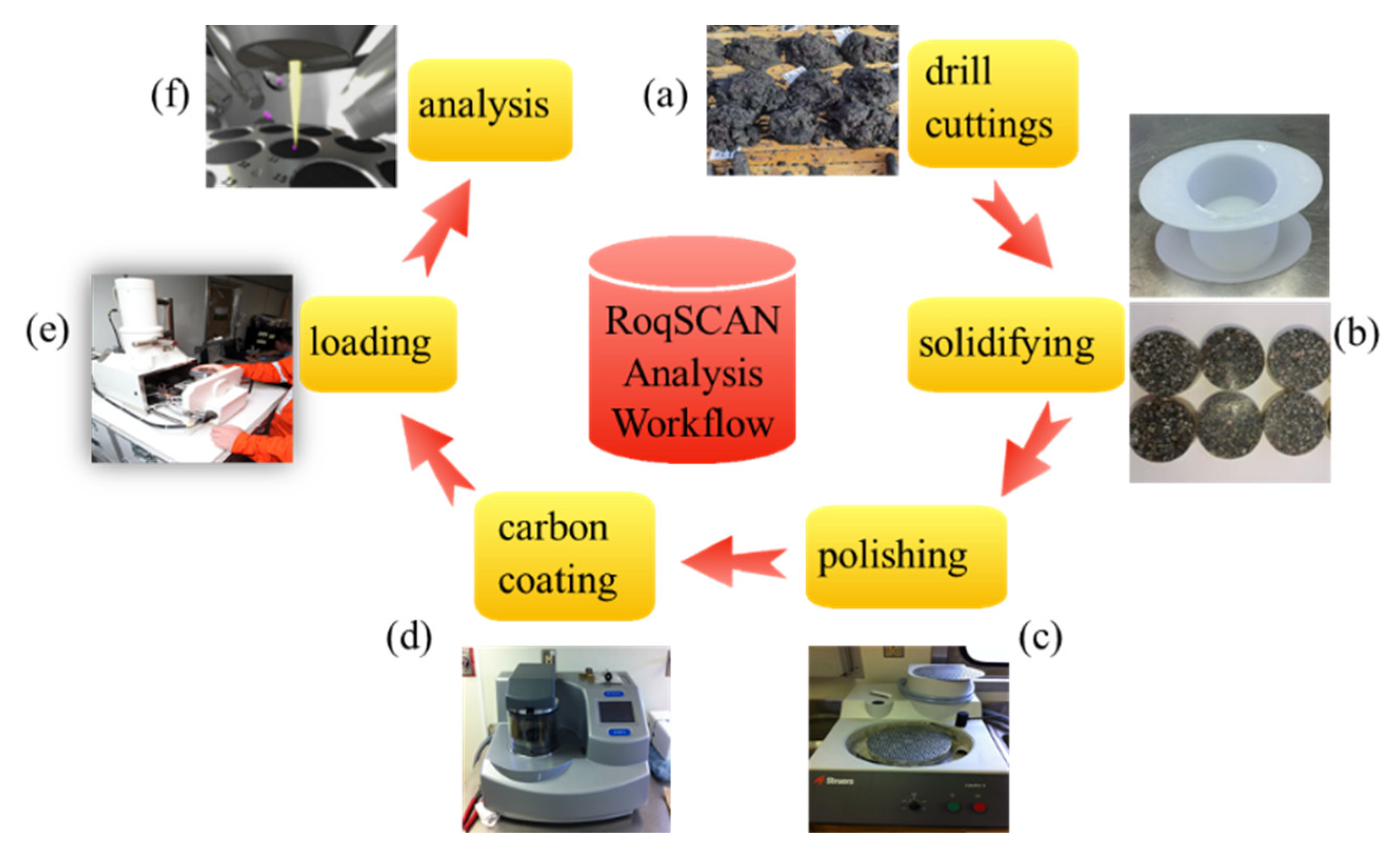
Figure 1. Workflow of drill cutting scanning.
Processes 11 00835 g001
Reservoir rocks are composed of minerals, pores, microfractures, and fluids [33,34,35], and many scholars have proven that mineral compositions and pore characteristics are the key factors affecting Vs [36,37,38]. Moreover, the S-wave does not propagate in the reservoir fluids [39]. Therefore, drill cuttings can be used to characterize all mineral and pore information of the reservoir; they can be used to predict Vs. There are fewer voices to question that drill cuttings reflect the mineral characteristics of the reservoir, and yet some scholars questioned that the small cutting size may not be representative of the formation rock pore system. In response to the question, Singer et al. [40] present experimental evidence to show that cuttings > 2 mm retain all porosity information. In summary, the mineral and pore information provided by drill cuttings can be used to predict Vs. With the help of the RoqSCAN technique, mineralogical information is able to achieve under EDS (Figure 2), and pore information can be obtained under SEM (Figure 3). The mineralogical information is characterized by mineral type and content, and pore information is characterized by the void area ratio and void aspect ratio. Void area ratio refers to the visible porosity of the rock under SEM (i.e., the percentage of the void area over the total area of the observed field of view), and void aspect ratio refers to the ratio between the minor and major axes of an ellipsoidal pore [10].

2.2. The Proposed CNN-SGRU Model

Machine learning algorithms have proven to be efficient and effective in predicting Vs from petrophysical logging data with their black-box nonlinear mapping ability [23]. In this work, we proposed a novel deep learning model for automatic Vs estimation using a Convolutional neural network (CNN) and Stacked gated recurrent unit (SGRU) combined neural network (CNN-SGRU). This hybrid model can deeply mine the inner correlations between drill cutting features and Vs for more robust and accurate predictions.

2.2.1. Convolutional Neural Network (CNN)

CNN implements feature extraction from input data by virtue of a local connection, weight sharing, and translation invariance, promoting its wide application in face recognition [41], sentiment analysis [42], and time series forecasting [43]. As shown in Figure 4, CNN generally comprises several iterations of convolution layers, a pooling layer, and a dense layer. Among them, convolution layers obtain abstract features from multidimensional data through the inner product of the input and convolution kernel. Playing the role of downsampling, the pooling layer is responsible for reducing the size of extracted feature maps by replacing the values within the sliding window with statistical values (e.g., average or max), so as to eliminate the effect of interference and noise and save computational resources. Located after the convolutional and pooling layers, the dense layer is a selectively added component, which is used to connect the obtained features with the target and thus output forecasts. Based on layers with diverse functions, CNN is capable of extracting features effectively while reducing the dimension of input data, which is beneficial to prediction performance and efficiency.

2.2.2. Stacked Gated Recurrent Unit (SGRU)

Well logging, Vs, and drill cuttings are typical sequential data that vary with depth, which can reflect the variances in formation and lithology. As a popular machine learning algorithm, the Recurrent neural network (RNN) is an expert in handling sequences because it can not only relate the output with input features but also associate the output of the current step with previous steps. In the past decades, RNN and its variants, such as Long short-term memory (LSTM) and Gated recurrent unit (GRU), have been successfully used in sequence processing and forecasting, such as speech recognition [44], machine translation [45], power forecasting [46], and traffic flow estimation [47]. By comparison, GRU introduces a gate mechanism to avoid the issue of gradient exploding and vanishing RNN, and further simplifies the gate structure of LSTM for greater efficiency, making itself stand out.
As the forecasting task becomes more complex and challenging, it is found that deep neural networks contribute to obtaining better performance. By stacking multiple layers of neural networks, deep neural networks can recombine the learned features from the previous layers and create high-level abstract features. One layer disposes of part of the task at hand and then passes the information to the next layer. Acting as a processing pipeline, deep neural networks can be exponentially more efficient at capturing representations combined with shallow models. Therefore, a Stacked gated recurrent unit (SGRU) is adopted as a basic component in this work to perform sequence forecasting.
In an SGRU neural network, multiple GRU hidden states are stacked on top of each other, which allows information to be learned at different scales and levels, as shown in Figure 5a. Figure 5b depicts the inner cell structure of the GRU cell. The cell state controls the information flow among different steps, expressed as:
h T = ( 1 z T ) h T - 1 + z T h ˜ T
where hT−1 and hT are the hidden states at steps T−1 and T, respectively. ZT denotes the update gate and h ˜ T is the candidate’s hidden state, which can be calculated by:
z T = σ ( w z [ h T - 1 , X T ] + b z )
h ˜ T = tanh ( w h [ h T - 1 · r T , X T ] + b h )
where σ is a sigmoid activation function and tanh is a tanh activation function. wz and bz are the weight and bias of the update gate. wh and bh are the weight and bias of the candidate’s hidden state. XT represents the input at step T. rT represents an important gate, namely the reset gate, which can be determined by:
r T = σ ( w r [ h T - 1 , X T ] + b r )
where wr and br are the weight and bias of the reset gate.
Based on the above calculation process, the input of the current step and the output of the previous steps interact with the cell state through the reset gate and upset gate. The forecast of the current step is the output, which will influence the output of the next steps.

2.2.3. CNN-SGRU Model

Based on CNN and SGRU, a novel CNN-SGRU deep learning model is built for Vs forecasting using drill cutting data, which combines the strengths of CNN and SGRU for better performance. Figure 6 shows the structure of the proposed CNN-SGRU model. The CNN component comprises two layers of one-dimensional CNN (1D CNN), Batch normalization, and Max pooling, which assists in capturing effective spatial representations from massive input data while accelerating feature extraction. Among them, 1D CNN layers are primarily responsible for abstract feature extraction. Batch normalization and Max pooling layers are added to save computational resources. Then the extracted features by CNN are passed to the SGRU component for further relationship mapping between rock microstructure and Vs. Three layers of GRU constitute the SGRU. The dropout layer is added to avoid overfitting problems in deep learning. Finally, the forecast is output through a dense layer.

2.3. Evaluation Indices

To quantitatively evaluate the prediction performance, three common indices are employed in this work, including Mean absolute percentage error (MAPE), Root mean square error (RMSE), and Mean absolute error (MAE). Bigger values of MAPE, RMSE, and MAE mean bigger prediction errors and lower accuracy.
  • (a) MAPE is utilized to show the proportion of prediction errors to true values, calculated by:
    MAPE = 1 M i = 1 M y i p y i t y i t × 100 %
    where y i p and y i t are the predicted and the true values of the ith sample, respectively. M denotes the number of samples.
  • (b) RMSE is used to compute the standard deviation between predictions and actual values, as below:
    RMSE = i = 1 M ( y i t y i p ) 2 M
  • (c) MAE represents the average difference between the forecasts and actual values, which is calculated by:
    MAE = 1 M i = 1 M y i t y i p

2.4. Overall Workflow

Figure 7 describes the overall workflow of the S-wave prediction process. A total of five steps are listed in detail.
  • Step 1: Data preparation. First, mineralogical and pore information are acquired using RoqSCAN, then the Pearson correlation [48] is used to analyze the main control factors affecting Vs, and finally, the main control factors are used as model input parameters.
  • Step 2: Data preprocessing. To prepare adequate data for model training, obtained data have to be preprocessed in advance, including Z-score normalization (Equation (8)) and input-output pair transformation. Z-score normalization facilitates the convergence of deep neural networks. A sliding window is utilized to transform input and output data into 3D input-2D output pairs. A more detailed transformation process can refer to [21].
    x ˜ = x x ¯ δ
    where x and x ˜ are the raw data and the normalized data, respectively. x ¯ and δ are the average and standard deviation of x, respectively.
  • Step 3: Data partition. The whole dataset is divided into the training set, validation set, and test set in the ratio of 70%, 15%, and 15% with sampling depth.
  • Step 4: Hyperparameter optimization. Optimal hyperparameters of the CNN-SGRU model are determined through the Bayesian optimization algorithm, such as the number of neurons, learning rate, and dropout ratio.
  • Step 5: Model training and forecasting. With drill cutting features as inputs, the CNN-SGRU model is well-trained for Vs forecasting based on the optimal hyperparameters.
Figure 7. Overall workflow of the Vs prediction.
Processes 11 00835 g007

3. Results

In this section, the proposed CNN-SGRU hybrid model is used for Vs prediction in a horizontal well, the whole prediction process is introduced in detail, and the prediction results are compared with the rock physics model (Xu-White model) and single neural networks (CNN and GRU).

3.1. Data Preparation and Preprocession

The study area is located on the west slope of the Mahu Depression in the Junggar Basin, China, where the Lower Triassic Baikouquan Formation is dominated by coarse clastic sediments and belongs to the fan delta-lake sedimentary system, and the main rock type is glutenite. The target well is a horizontal well (MaX) with a horizontal section of 945 m, and Vs logging is carried out in this well. The interval of drill cutting sampling was <2 m, and a total of 524 samples were taken. Mineral and pore information for each sample was obtained by Roqscan, and minerals were divided into four main categories: siliciclastics, clays, carbonates, and accessory minerals. Figure 8 shows the distribution of different types of minerals in the horizontal section of MaX, the minerals in drill cuttings are mainly siliciclastics and clays. In addition, siliciclastic compositions are mainly quartz and albite as shown in Figure 9. Figure 10 illustrates the void area ratio and void aspect ratio of drill cuttings, and there is a large fluctuation of the void area ratio with depth. By comparison, the aspect ratio is stable at about 0.1. As shown in Figure 11, Pearson correlation analysis shows the correlation between drill cutting characteristics parameters and the testing Vs, and comparatively, siliciclastics, clays, quartz, and void area ratio are strongly correlated with Vs. To reduce the complexity of the proposed model, prevent the influence of redundant features, and improve the calculation speed and accuracy, siliciclastic content, clay content, quartz content, and void area ratio are chosen as model inputs.
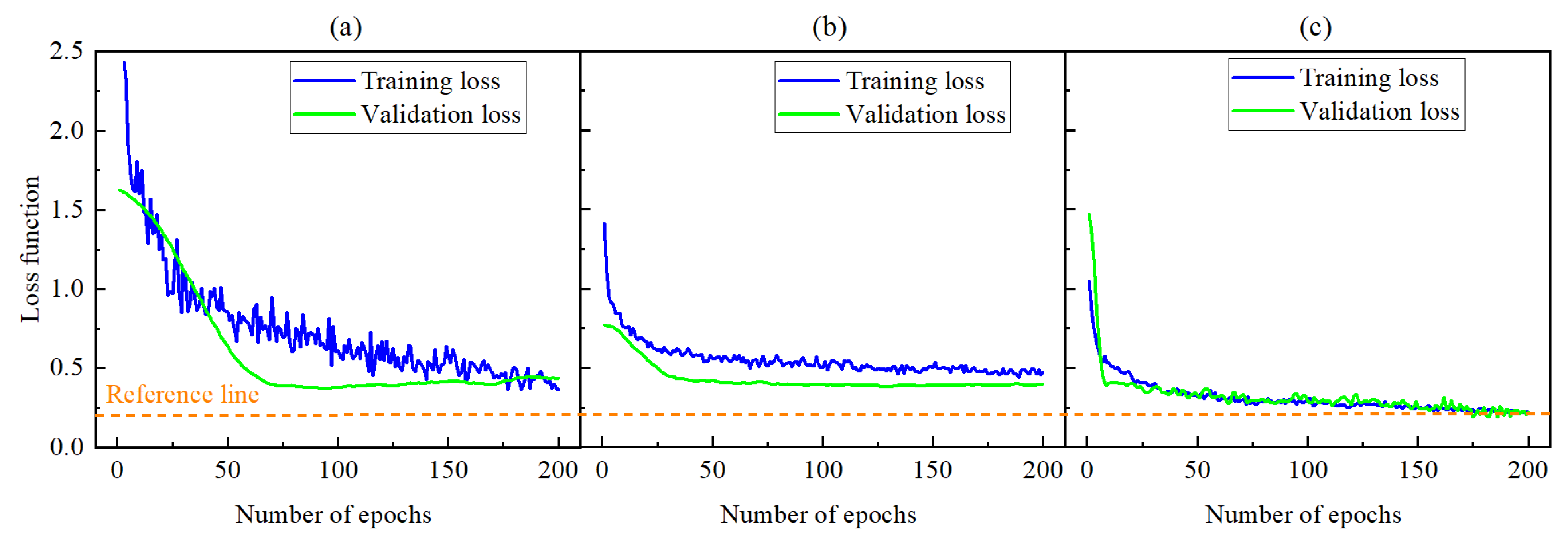
The collected input data cannot be fed directly into the proposed model and need to be processed. First, obtained data had to be preprocessed, including Z-score normalization and input-output pair transformation, and then the dataset was divided into the training set, validation set, and test set. Finally, hyperparameters were optimized by the Bayesian optimization algorithm. Table 1 shows the optimal values of hyperparameters used in the CNN-SGRU hybrid model and comparative models (CNN and GRU). All the models were coded in Python 3.7 under the Keras framework [49] and run on Intel ® Core™ 16 i7-4790 3.60 GHz CPU with 16 GB of memory. Training error curves of CNN, GRU, and CNN-SGRU models are shown in Figure 12. Figure 12 shows that the CNN-SGRU model obtains a more desirable training error curve, and the loss function error is minimal. MAPE, RMSE, and MAE were used as evaluation criteria.

3.2. Comparison of Prediction Accuracy Analysis

To verify the feasibility and accuracy of the proposed CNN-SGRU hybrid model, the Vs prediction results are compared with the Xu-White model, CNN, and GRU. The theories and methodologies of CNN and GRU are introduced in Section 2, and the Xu-White model in this study is an approximation model proposed by Keys and Xu [50] in 2002. Figure 13 is the workflow of the petrophysical model, the specific modeling process consists of two steps:
  • (a) calculating the modulus of the matrix of different minerals with the V-R-H model [51]. In Equations (9) and (10), the mineral modulus values refer to [52,53].
  • (b) Based on K-T theory [2], the modulus of dry rock can be calculated by Equations (11) and (12), and then Vs can be calculated by Equation (13).
K m = i = 1 N f i K i + i = 1 N f i K i 1 2
μ m = i = 1 N f i μ i + i = 1 N f i μ i 1 2
K ( ϕ ) = K m ( 1 ϕ ) p
μ ( ϕ ) = μ m ( 1 ϕ ) q
V s = μ / ρ
where K m and μ m are the matrix bulk modulus and shear modulus, respectively. f i , K i and μ i are volume content, bulk modulus and shear modulus of the i-th mineral component, respectively. N is the number of different mineral types. K ( ϕ ) and μ ( ϕ ) are bulk modulus and shear modulus of dry rock, respectively. ϕ is the porosity. P and q are the geometrical factors, respectively. ρ is dry rock density.
Figure 13. Schematic diagram of the rock physics model.
Processes 11 00835 g013
Figure 14 shows the Vs prediction results of the Xu-White model, CNN, GRU, and the proposed CNN-SGRU model. As shown in Figure 14a, overall, the predicted Vs curve of the Xu-White method is similar to the trend of the testing Vs curve, but the local matching degree is not good. The reason for this result is that the Xu-White model is mainly applicable to sandstone, while glutenite is a special sedimentary rock. The existence of gravel in glutenite enhances the heterogeneity of glutenite, which ultimately leads to some deviations in the prediction results. Compared with the GRU and CNN-SGRU, CNN learns better for the fluctuation of data curves and can better extract the dramatic fluctuations between data, as shown in Figure 14b–d. On the whole, the results of the CNN, GRU, and CNN-SGRU are acceptable for the training set. However, the result of GRU for the test set is an obvious error, which implies that the generalizability is not strong enough to predict the data that did not appear during training. In contrast, the proposed CNN-SGRU hybrid model has a good prediction for both the training set and test set, and it learns the inner variation mechanism, as shown in Figure 14d.
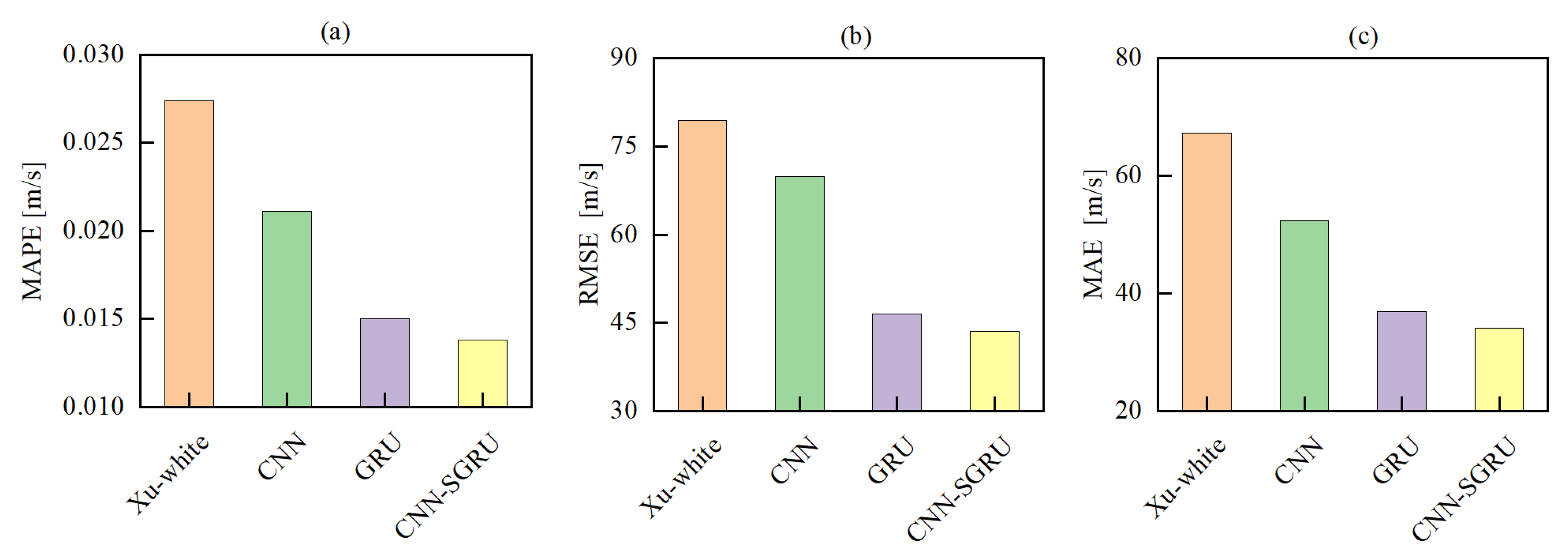
The prediction effect of the test set best reflects the performance of the model, so the test set needs to be further analyzed. Figure 15 shows the results of the evaluation indices of the four methods, Figure 16 is the relative error distribution of the four methods, and the values of the evaluation indices are shown in Table 2. Both statistical analysis results of Figure 15 and Figure 16 reveal that the proposed method exhibited the optimum performance. The MAPE, RMSE, and MAE of the CNN-SGRU model are 0.01381, 43.4676, and 34.04062, respectively. By comparison, the evaluation indices of the Xu-white model are 0.02739, 79.42729, and 67.25988, respectively. The predicted results demonstrate that the machine learning prediction method outperforms the rock physics modeling method. The evaluation indices of the CNN-SGRU are reduced by 34~37% and 6~8% compared to CNN and GRU, respectively. The CNN has the largest relative error interval, and the CNN-SGRU has the smallest, as shown in Figure 16. This means that CNN has lower prediction accuracy despite better learning curve fluctuations. Compared with CNN, the prediction error fluctuation interval of GRU is smaller, but the mean and median relative error of GRU is larger. The CNN-SGRU hybrid model retained not only the advantages of the CNN in complex feature extraction but also those of SGRU in time-series feature extraction, this is to say, hybrid neural networks can combine the advantage of single neural networks. The CNN-SGRU hybrid model has the smallest relative error interval, mean relative error, and intermediate relative error. In summary, the proposed method achieved the optimum Vs prediction based on the drill cutting data.

4. Discussion

The current study proposed a hybrid neural networks model (CNN-SGRU model) to predict Vs, and the input to the model is not the conventional log data but drill cutting features. The graphical correlation between target data and predicted outputs of the models is shown in Figure 14 for training and testing data, and Table 2 provides a comparison between all models used based on the statistical evaluation indices including Mean absolute percentage error (MAPE), Root mean square error (RMSE), and Mean absolute error (MAE). These results show a significant improvement in the CNN-SGRU hybrid model in comparison with the conventional rock physics model (Xu-White model), CNN, and GRU models. Although the hybrid model has obtained better prediction results, it still has some limitations to improve. Next, the prediction accuracy can be further improved in the following ways:
  • (a) Optimizing drill cutting sampling interval. The conventional log sampling interval is about 0.125 m, while the drill cutting sampling interval is 2 m, which is much larger than the log sampling interval, so it may lead to larger fluctuations and reduce the prediction accuracy.
  • (b) Finding new optimization algorithms. In the future, this method can be combined with the optimization algorithms to enhance the accuracy of the model, such as the Shrimp and Goby Association Search algorithm (SGA) [54], Grey Wolf Optimizer (GWO) algorithm [55], surrogate-assisted stochastic optimization inversion (SASOI) algorithm [56] and so on.
  • (c) Improving model generalization capabilities. The current study only focuses on glutenite reservoirs, and there is a need to analyze the effectiveness of the proposed model in other types of reservoirs.

5. Conclusions

In this work, a novel CNN-SGRU hybrid model for Vs forecasting is proposed, which can output more accurate, robust, and generalizable forecasts by fully leveraging the strengths of CNN and SGRU. The CNN module is responsible for extracting the spatial features from sequences and SGRU is employed to find the temporal features embedded in Vs variation. In this way, more important spatiotemporal features are highlighted, leading to a performance boost.
A studied well case was elaborated, and the results show that the prediction results of the CNN-SGRU model are the most consistent with the actual Vs values, and the CNN-SGRU model outperforms the conventional petrophysical model (Xu-White model), CNN and GRU models in terms of both forecasting accuracy and stability. The MAPE, RMSE, and MAE of the CNN-SGRU model are 0.01381, 43.4676, and 34.04062, respectively. The mean relative error of the Xu-white model, CNN, GRU, and CNN-SGRU is 2.43%, 0.30%, 0.54%, and 0.05%, respectively. Additionally, drill cuttings can reflect the mineral and pore information of the reservoir, therefore, Vs can be forecast well by drill cuttings as model inputs.

Author Contributions

Conceptualization, methodology, writing, F.X.; writing- reviewing and editing, resources, X.L.; writing- reviewing and editing and funding acquisition, S.Z. All authors have read and agreed to the published version of the manuscript.

Funding

This work was supported by the PetroChina Strategic Cooperation Science and Technology Project (Grant No. ZLZX2020-01-04).

Institutional Review Board Statement

Not applicable.

Informed Consent Statement

Not applicable.

Data Availability Statement

The raw data required to reproduce these findings cannot be shared at this time as they also form part of an ongoing study.

Conflicts of Interest

The authors declare no conflict of interest.

References

  1. Buland, A.; Omre, H. Bayesian linearized AVO inversion. Geophysics 2003, 68, 185–198. [Google Scholar] [CrossRef] [Green Version]
  2. Mavko, G.; Mukerji, T.; Dvorkin, J. The Rock Physics Handbook: Tools for Seismic Analysis of Porous Media; Cambridge University Press: Cambridge, UK, 2009. [Google Scholar]
  3. Wang Jun Cao, J.; Yuan, S. Shear wave velocity prediction based on adaptive particle swarm optimization optimized recurrent neural network. J. Pet. Sci. Eng. 2020, 194, 107466. [Google Scholar] [CrossRef]
  4. Gholami, R.; Moradzadeh, A.; Rasouli, V.; Hanachi, J. Shear wave velocity prediction using seismic attributes and well log data. Acta Geophys. 2014, 62, 818–848. [Google Scholar] [CrossRef] [Green Version]
  5. Sohail, G.M.; Hawkes, C.D. An evaluation of empirical and rock physics models to estimate shear wave velocity in a potential shale gas reservoir using wireline logs. J. Pet. Sci. Eng. 2020, 185, 106666. [Google Scholar] [CrossRef]
  6. Castagna, J.P. Relationships between compressional-wave and shear-wave velocities in clastic silicate rocks. Geophysics 1985, 50, 530–743. [Google Scholar] [CrossRef]
  7. Greenberg, M.L.; Castagna, J.P. Shear-Wave Velocity Estimation in Porous Rocks: Theoretical Formulation, Preliminary Verification and Applications1. Geophys. Prospect. 1992, 40, 195–209. [Google Scholar] [CrossRef]
  8. Wyllie, M.; Gregory, A.R.; Gardner, G. An experimental investigation of factors affecting elastic wave velocities in porous media. Geophysics 1958, 23, 459–493. [Google Scholar] [CrossRef]
  9. De-hua Han Nur, A.; Morgan, D. Effects of Porosity and Clay Content on Wave Velocities in Sandstones. Geophysics 1986, 51, 2093–2107. [Google Scholar]
  10. Xu, S.; White, R.E. A physical model for shear-wave velocity prediction. Geophys. Prospect. 1996, 44, 687–717. [Google Scholar] [CrossRef]
  11. Kumar, M. Pore shape effect on elastic properties of carbonate rocks. SEG Tech. Program Expand. Abstr. 2005, 24, 1949–4645. [Google Scholar]
  12. Azadpour, M. Rock physics model-based prediction of shear wave velocity utilizing machine learning technique for carbonate reservoir. J. Pet. Sci. Eng. 2020, 195, 107864. [Google Scholar] [CrossRef]
  13. Xu, S.; Payne, M.A. Modeling elastic properties in carbonate rocks. Lead. Edge 2009, 28, 1–128. [Google Scholar] [CrossRef]
  14. Zhang, B.; Jin, S.; Liu, C.; Guo, Z.; Liu, X. Prediction of shear wave velocity based on a statistical rock-physics model and Bayesian theory. J. Pet. Sci. Eng. 2020, 195, 107710. [Google Scholar] [CrossRef]
  15. Mendi, A.F. A Sentiment Analysis Method Based on a Blockchain-Supported Long Short-Term Memory Deep Network. Sensors 2022, 22, 4419. [Google Scholar] [CrossRef] [PubMed]
  16. Al-Anazi, A.F.; Gates, I.D. Support vector regression to predict porosity and permeability: Effect of sample size. Comput. Geosci. 2012, 39, 64–76. [Google Scholar] [CrossRef]
  17. Pan, S.; Zheng, Z.; Guo, Z.; Luo, H. An optimized XGBoost method for predicting reservoir porosity using petrophysical logs. J. Pet. Sci. Eng. 2022, 208, 109520. [Google Scholar] [CrossRef]
  18. Zhao, X.; Chen, X.; Qiao, H. Logging-data-driven permeability prediction in low-permeable sandstones based on machine learning with pattern visualization: A case study in Wenchang A Sag, Pearl River Mouth Basin. J. Pet. Sci. Eng. 2022, 214, 110517. [Google Scholar] [CrossRef]
  19. Gu, Y.; Zhang, D.; Bao, Z. Lithological classification via an improved extreme gradient boosting: A demonstration of the Chang 4+5 member, Ordos Basin, Northern China. J. Asian Earth Sci. 2021, 215, 104798. [Google Scholar] [CrossRef]
  20. Agbaji, A.L. An Empirical Analysis of Artificial Intelligence, Big Data and Analytics Applications in Exploration and Production Operations. In Proceedings of the International Petroleum Technology Conference, 2021, Virtual, 23 March–1 April 2021. [Google Scholar]
  21. Li, X.; Ma, X.; Xiao, F.; Xiao, C.; Wang, F.; Zhang, S. Time-series production forecasting method based on the integration of Bidirectional Gated Recurrent Unit (Bi-GRU) network and Sparrow Search Algorithm (SSA). J. Pet. Sci. Eng. 2022, 208, 109309. [Google Scholar] [CrossRef]
  22. Li, X.; Ma, X.; Xiao, F.; Xiao, C.; Wang, F.; Zhang, S. Multistep Ahead Multiphase Production Prediction of Fractured Wells Using Bidirectional Gated Recurrent Unit and Multitask Learning. SPE J. 2023, 28, 381–400. [Google Scholar] [CrossRef]
  23. Zhang, Q.Y. Improvement of petrophysical workflow for shear wave velocity prediction based on machine learning methods for complex carbonate reservoirs. J. Pet. Sci. Eng. 2020, 192, 107234. [Google Scholar] [CrossRef]
  24. Zhang, Y.; Zhang, C.; Ma, Q.; Zhang, X.; Zhou, H. Automatic prediction of shear wave velocity using convolutional neural networks for different reservoirs in Ordos Basin. J. Pet. Sci. Eng. 2021, 208, 109252. [Google Scholar] [CrossRef]
  25. Park, J.Y.; Sim, S.H.; Yoon, Y.G.; Oh, T.K. Prediction of Static Modulus and Compressive Strength of Concrete from Dynamic Modulus Associated with Wave Velocity and Resonance Frequency Using Machine Learning Techniques. Materials 2020, 13, 2886. [Google Scholar] [CrossRef] [PubMed]
  26. Li, X.; Ma, X.; Xiao, F.; Xiao, C.; Wang, F.; Zhang, S. Intelligence-Driven Prediction of Shear Wave Velocity Based on Gated Recurrent Unit Network. In Proceedings of the 56th U.S. Rock Mechanics/Geomechanics Symposium, Santa Fe, NM, USA, 26–29 June 2022. [Google Scholar]
  27. Wang, J.; Cao, J.; Yuan, S.; Zhou, X.; Zhou, P. Spatiotemporal Synergistic Ensemble Deep Learning Method and Its Application to S-Wave Velocity Prediction. IEEE Geosci. Remote Sens. Lett. 2021, 19, 8024705. [Google Scholar] [CrossRef]
  28. Wang, J.; Cao, J.; Zhao, S.; Qi, Q. S-wave velocity inversion and prediction using a deep hybrid neural network. Sci. China Earth Sci. 2022, 65, 18. [Google Scholar] [CrossRef]
  29. Xiao, F.; Zhang, S.; Li, X.; Ma, X. Perforation Location Optimization Considering Microscopic Structure for Multi-Cluster Fracturing Technology. In Proceedings of the 56th U.S. Rock Mechanics/Geomechanics Symposium, Santa Fe, NM, USA, 26–29 June 2022. [Google Scholar]
  30. Tom, A.; Vinh, L.C.; Graham, S.; Oliver, G. Portable Technology Puts Real-time Automated Mineralogy on the Well Site. In Proceedings of the SPE Unconventional Resources Conference and Exhibition-Asia Pacific, Brisbane, Australia, 11–13 November 2013. [Google Scholar]
  31. Khodaei, A.; Lee, H.; Banaei-Kashani, F.; Shahabi, C.; Ershaghi, I. A Mutual Information-Based Metric for Identification of Nonlinear Injector Producer Relationships in Waterfloods. In Proceedings of the SPE Western Regional Meeting 2009, San Jose, CA, USA, 24–26 March 2009. [Google Scholar]
  32. Castillo, G.; Chesser, K.; Bouziat, A.; Oliver, G.; Ly, C.V.; Kuo, L.; Bathellier, E. Integrating Active and Passive Seismic Data to Better Predict Hydraulic Fracturing. In Proceedings of the SPE/CSUR Unconventional Resources Conference, 2014, Calgary, AB, Canada, 30 September–2 October 2014. [Google Scholar]
  33. Li, Y. A rock physics model for the characterization of organic-rich shale from elastic properties. Pet. Sci. 2015, 12, 264–272. [Google Scholar] [CrossRef] [Green Version]
  34. Gp, A.; Cr, B. An efficient rock-physics workflow for modeling and inversion in anisotropic organic-shales. J. Pet. Sci. Eng. 2019, 180, 1101–1111. [Google Scholar]
  35. Li, Y.; Chen, J.; Elsworth, D.; Pan, Z.; Ma, X. Nanoscale mechanical property variations concerning mineral composition and contact of marine shale. Geosci. Front. 2022, 13, 101405. [Google Scholar] [CrossRef]
  36. Tutuncu, A.N.; Podio, A.L.; Sharma, M.M. An experimental investigation of factors influencing compressional- and shear-wave velocities and attenuations in tight gas sandstones. Geophysics 1994, 59, 77–86. [Google Scholar] [CrossRef]
  37. Smith, T.M.; Sayers, C.M.; Sondergeld, C.H. Rock Properties In Low-porosity/low-permeability Sandstones. Geophys. Lead. Edge Explor. 2009, 28, 1–128. [Google Scholar] [CrossRef]
  38. Chen, S.; Lan, H.; Zhao, H.; Zhang, T. A rock physics model for tight glutenite reservoir. In Proceedings of the SEG 2018 Workshop: Reservoir Geophysics, Daqing, China, 5–7 August 2018. [Google Scholar]
  39. Gassmann, F. Elasticity of Porous Media [Uber die elastizitat poroser medie]. Viertelijahrsschrift Nat. Gesselschaft 1951, 96, 1–23. [Google Scholar]
  40. Gabriela, S.; Mark, F.; Chen, S.; Ma, S.M. NMR Drill Cutting Analysis: Methodology Evaluation and Operational Best Practices. In Proceedings of the SPWLA 62nd Annual Logging Symposium, Virtual Event, 17–20 May 2021. [Google Scholar]
  41. Chopin, J.; Fasquel, J.B.; Mouchère, H.; Dahyot, R.; Bloch, I. Model-based inexact graph matching on top of CNNs for semantic scene understanding. arXiv 2023, arXiv:2301.07468. [Google Scholar]
  42. Venkatesh Hegde, S.U.; Basapur, S.B. DistilBERT-CNN-LSTM Model with GloVe for Sentiment Analysis on Football Specific Tweets. IAENG Int. J. Comput. Sci. 2022, 2 Pt 2, 49. [Google Scholar]
  43. Li, X.; Ma, X.; Xiao, F.; Xiao, C.; Wang, F.; Zhang, S. Small-Sample Production Prediction of Fractured Wells Using Multitask Learning. SPE J. 2022, 27, 1504–1519. [Google Scholar] [CrossRef]
  44. Kumar, L.A.; Renuka, D.K.; Rose, S.L.; Shunmuga Priya, M.C.; Wartana, I.M. Deep learning based assistive technology on audio visual speech recognition for hearing impaired. Int. J. Cogn. Comput. Eng. 2022, 3, 24–30. [Google Scholar] [CrossRef]
  45. Nouhaila, B.; Habib, A.; Abdellah, A.; Farouk, A.I.E. LSTM or GRU for Arabic machine translation? Why not both! Ibn el farouk Abdelhamid Teaching, Languages and Cultures Laboratory Mohammedia. In Proceedings of the 8th International Conference on Innovation and New Trends in Information Technology, Stockholm, Sweden, 23–25 July 2021. [Google Scholar]
  46. He, H.; Wang, H.; Ma, H.; Liu, X.; Jia, Y.; Gong, G. Research on Short-term Power Load Forecasting Based on Bi-GRU. J. Phys. Conf. Ser. 2020, 1639, 012017. [Google Scholar] [CrossRef]
  47. Zhang, M.; Wang, X. Traffic time prediction of urban main road based on GRU-RNN model. J. Beijing Inf. Sci. Technol. Univ. 2019, 34, 30–35. [Google Scholar]
  48. Okoli, P.; Vega, J.C.; Shor, R. Estimating Downhole Vibration via Machine Learning Techniques Using Only Surface Drilling Parameters. In Proceedings of the SPE Western Regional Meeting, 2019, San Jose, CA, USA, 23–26 April 2019. [Google Scholar]
  49. Li, X.; Ma, X.; Xiao, F.; Wang, F.; Zhang, S. Application of Gated Recurrent Unit (GRU) Neural Network for Smart Batch Production Prediction. Energies 2020, 13, 6121. [Google Scholar] [CrossRef]
  50. Keys, R.G.; Xu, S. An approximation for the Xu-White velocity model. Geophysics 2002, 67, 1406–1414. [Google Scholar] [CrossRef]
  51. Hill, R. The elastic behavior of crystalline aggregate. Proc. Phys. Soc. Sect. 1952, A65, 5. [Google Scholar]
  52. Sun, W.; Zuo, Y.; Wu, Z.; Liu, H.; Zheng, L.; Shui, Y.; Xi, S.; Lou, Y.; Luo, X. The distribution characteristics of brittle minerals in the Lower Cambrian Niutitang Formation in northern Guizhou. J. Nat. Gas Sci. Eng. 2020, 86, 103752. [Google Scholar] [CrossRef]
  53. Jia, Y.; Tang, J.; Lu, Y.; Lu, Z. Laboratory geomechanical and petrophysical characterization of Longmaxi shale properties in Lower Silurian Formation, China. Mar. Pet. Geol. 2020, 124, 104800. [Google Scholar] [CrossRef]
  54. Sang-To, T.; Le-Minh, H.; Wahab, M.A.; Thanh, T.-C. A new metaheuristic algorithm: Shrimp and Goby association search algorithm and its application for damage identification in large-scale and complex structures. Adv. Eng. Softw. 2023, 176, 103363. [Google Scholar] [CrossRef]
  55. Sang-To, T.; Le-Minh, H.; Mirjalil, S.; Wahab, M.A.; Cuong-Le, T. A new movement strategy of grey wolf optimizer for optimization problems and structural damage identification. Adv. Eng. Softw. 2022, 173, 103276. [Google Scholar] [CrossRef]
  56. Li, Y.; Amin Hariri-Ardebili, M.; Deng, T.; Wei, Q. A surrogate-assisted stochastic optimization inversion algorithm: Parameter identification of dams. Adv. Eng. Inform. 2023, 55, 101853. [Google Scholar] [CrossRef]
Figure 2. Mineral distribution under EDS.
Processes 11 00835 g002
Figure 3. Pore morphology under SEM.
Processes 11 00835 g003
Figure 4. Sketch of the structure of CNN.
Processes 11 00835 g004
Figure 5. Sketch of the SGRU neural network: (a) structure of SGRU, (b) inner cell structure of GRU.
Processes 11 00835 g005
Figure 6. Structure of the proposed CNN-SGRU model.
Processes 11 00835 g006
Figure 8. Area map of mineral composition of drill cuttings at different well depths.
Processes 11 00835 g008
Figure 9. Stacked area map of the distribution of silicate mineral types at different well depths.
Processes 11 00835 g009
Figure 10. Scatter plot of drill cutting pore information at different well depths.
Processes 11 00835 g010
Figure 11. Heatmap of Pearson correlation analysis.
Processes 11 00835 g011
Figure 12. The variation of the loss function with training epoch: (a) CNN, (b) GRU, (c) CNN-SGRU.
Processes 11 00835 g012
Figure 14. Comparison between actual and prediction Vs of the four models.
Processes 11 00835 g014aProcesses 11 00835 g014b
Figure 15. Comparison of performance of four models in terms of (a) MAPE, (b) RMSE, and (c) MAE.
Processes 11 00835 g015
Figure 16. Boxplots of relative error of the four models.
Processes 11 00835 g016
Table 1. Optimization range and optimal values of hyperparameters.
HyperparameterOptimization RangeOptimal Values
Number of Conv1D layers[1, 4]2
Number of BiGRU layers[2, 5]3
Number of neurons in Conv1D layers[10, 100]50
Number of neurons in BiGRU layers[10, 100]63
Activation functiontanh, Relu, sigmoidRelu
Dropout rate[0.1, 0.5]0.2
Learning rate[0.0001, 0.01]0.0015
Size of the input window[3, 28]3
Table 2. Comparison of prediction errors of various models.
Prediction MethodEvaluation Indice
MAPE [m/s]RMSE [m/s]MAE [m/s]
Xu-white model0.0273979.4272967.25988
CNN0.0211269.8433752.33075
GRU0.0150446.408236.86077
CNN-SGRU0.0138143.4676634.04062
Disclaimer/Publisher’s Note: The statements, opinions and data contained in all publications are solely those of the individual author(s) and contributor(s) and not of MDPI and/or the editor(s). MDPI and/or the editor(s) disclaim responsibility for any injury to people or property resulting from any ideas, methods, instructions or products referred to in the content.