Abstract
Industrial processes often involve a long time delay, which adversely affects the stability of closed-loop control systems. The traditional Smith Predictor (SP) is a model-based controller used in processes with large time delays. The variation of system parameters and load disturbance situations are disadvantages of the traditional SP, and researchers have, therefore, proposed modified SP structures. In this paper, a design method based on the direct synthesis approach on a modified SP structure is discussed. In the design, an I-PD controller structure is used on the set-point tracking side of the SP, and a cascading PD lead–lag controller is used on the disturbance rejection side. In contrast with other studies in the literature, the use of simpler controllers enables the mathematical expressions that arise in the direct synthesis method to be significantly reduced. The proposed method is examined under the disturbance input effects for normal and parameter-changing conditions on system models with unstable second-order plus time-delay processes. The first plant model has two unstable poles, the second has one stable and one unstable pole, and the third has one unstable and one zero pole. When the results obtained using the proposed method were compared with other methods, significant improvements were achieved in terms of set-point tracking, disturbance rejection, and robustness conditions.
1. Introduction
Many industrial processes involve a long time delay, and this long delay is one of the barriers to the stabilization of closed-loop control systems. A long time delay significantly increases the phase delay of the system and, thus, affects the stability of closed-loop systems [1]. Traditional PID controllers are the most popular and widely used option because of their simplicity and ease of use, but it is difficult to control time-delayed operations using a conventional PID, as most industrial processes involve time delays [2].
It is much more difficult to design controllers for unstable processes than for stable processes because the closed-loop responses of unstable processes exhibit a large overshoot and settling time compared to stable processes. In addition, the design will be further constrained if the unstable process includes a zero in the right half plane and a time delay. For the control of unstable time-delayed systems, the PI-PD controller has been proposed as an alternative to conventional PID control [3,4,5,6]. In cases of disturbance input or parameter changes that affect the system, keeping the reference value and maintaining stability is another important problem. Furthermore, the destructive effects of these states become even more dominant in unstable time-delayed systems. This has led to the development of more effective control strategies. Various control strategies have been developed to reduce the problems caused by long delays, disturbances, and parameter changes in the control process. Model predictive controller (MPC), fuzzy logic controller (FLC), sliding mode control (SMC), internal model control (IMC), and Smith predictor (SP) methods are effective control strategies for minimizing the impact of these problems for stable and unstable systems.
The traditional SP is a model-based controller used in processes with large time delays. The SP was first proposed by Otto Smith in 1957 for the control of time-delayed stable systems. Later, it was developed for the control of unstable systems [7]. The SP has two loops—inner and outer. The inner loop has a core controller that can be easily designed to be free of dead time. The effects of load disturbance, time-delay, and modeling error (or parameter changes) in the system are suppressed by the controller used in the outer loop [8]. In the design phase of a traditional SP, the model and the time-delay component of the controlled system must be known. The efficiency of the SP decreases with modeling errors/uncertainties, internal/external disturbances, and delay variations [7].
To eliminate the disadvantages of SP, some researchers tried to make more effective performances by making some changes to the original structure of SP. In 1985, Palmor and Powers suggested that, by modifying the SP, regulatory capabilities for measurable disturbances could be improved. In their proposed structure, there is an additional tuning parameter to eliminate dead time [9]. Huang et al., for a modified Smith predictor, proposed a compensator that could predict the inverse of dead time at low frequencies, and they reported that it improved the disturbance rejection performance of the traditional SP [10]. Majhi and Atherton proposed a new Smith predictor structure, which separated the controller set-point response from the load response. They reported that their proposed SP structure delivered high performance for set-point response and load disturbance rejection in the control of an unstable time-delayed system and an integrating system with a long dead time [11]. In [12], Zhang et al. proposed an SP modification in which the set-point response and disturbance response of the closed loop system could be adjusted by two parameters. They reported that the two added tuning parameters could be optimized simultaneously. Kaya showed that the set-point and disturbance responses were improved when a PI-PD controller was used for the SP structure. They reported that the use of standard forms provided a simple algebraic approach to determining the parameters of the PI-PD controller [13]. In [14], Kaya focused on the design of a PI-PD controller for processes with high orders or long time delays. The PI-PD controller was designed to follow the response of a first or second-order plant, and simple adjustment formulas were therefore determined. Rao and Chidambaram proposed a modified form of the Smith predictor to control unstable second-order plus time-delay (USOPTD) processes, with and without a zero. In this structure, they used three controllers, and the synthesis method was used for controller design. They proposed analytical formulas for controllers. The method they proposed had two tuning parameters, and they also provided a set of guidelines for the selection of tuning parameters [15]. Uma and Rao proposed a modified Smith predictor design for the control of nonminimum-phase unstable second-order time-delay processes, with and without zero processes. The set-point tracking controller was a PID connected, in series, with a delay filter. The disturbance rejection controller was a PID connected, in series, with the lead–lag filter. The design of the set-point tracking controller and disturbance rejection controllers in their proposed SP involved use of the direct synthesis method, and they used set-point weighting to minimize overshoots [16]. Özbek and Eker proposed a modified SP based on a fractional fuzzy PI-PD. The performance of the proposed SP structure was investigated using real-time experiments on a time-delayed industrial air heating system [17]. In [18], Ajmeri and Ali proposed a modified Smith predictor for unstable time-delayed second-order processes. The proposed SP included three controllers: stabilizing (lead–lag compensator), set-point tracking (PI), and load disturbance rejection (PID controllers in cascade with a lead–lag filter). All three controllers were designed using a direct synthesis approach. All the controllers could be made with a single design parameter, which established a balance between performance and robustness. Additionally, appropriate tuning parameter values were recommended after examination of their effects on closed-loop performance and robustness. In [19], a generalization of the Smith Predictor was proposed to control linear time-invariant (LTI) and time-delayed single-input single-output (SISO) systems. To demonstrate the feasibility of the proposed approach, an experimental application was conducted. Espín et al. proposed a modified hybrid robust SP controller design for long-dead-time integrating systems. The proposed SP was a hybrid structure that combined sliding mode methodology, a Smith predictor build, and a PD controller [20]. A comparative study of Smith predictor structures was carried out by Mejía et al. [21]. This article compared three Smith predictor configurations and involved an experimental study. The controller parameters in the three SP control structures were adjusted using different optimization algorithms. The SP has also been used in many applications [22,23,24,25,26,27,28,29,30,31,32,33].
A well-designed controller should have good resistance to set-point tracking (or transient response), disturbance rejection, and parameter changes. Time-domain response methods and frequency-domain methods can be used for controller design. Controller parameters can be determined by analytical or iterative methods, using either time-domain features or frequency-domain features. Of the iterative methods, optimization approaches are generally used. In optimization approaches, an objective (or cost or fitness) function is determined according to the system parameters. Minimization or maximization of this function is achieved by changing the system parameters. In controller designs, the aim is to minimize or maximize the optimization function by changing the controller parameters. The optimization function is created according to the time or frequency characteristics of the controlled system. Performance criteria, such as integral absolute error (IAE), integral time absolute error (ITAE), integral square error (ISE), integral time square error (ITSE), transient and steady-state response values, and amplitude and phase margins of the controlled system, are widely used when defining the optimization function. In the literature, popular methods for controller design include genetic, particle swarm optimization, evolutionary development, artificial bee colony, ant colony, firefly, white whale, and gray wolf algorithms [34,35,36,37,38].
Other alternatives to optimization for controller design are classical analytical solution methods. In analytical solution methods, it is necessary to understand the mathematical model of the system to be controlled. Analytical methods are also carried out based on time-domain response or frequency-domain response properties. Most analytical designs use formulas for controller parameters, rise time, overshoot, settling time, and steady-state error values, which are the time-domain transient and steady-state characteristics of the system. Here, a desired reference output value of the system is known, and the controller parameters that can provide the transient and steady-state characteristics of this reference output are determined. Alternatively, the controller parameters can be understood by making use of the frequency characteristics of the specified reference model. In the direct synthesis (DS) method, the controller design is carried out over a plant model for which a closed-loop transfer function is sought [39]. In other words, the DS method relies on determining the desired system response and, then, identifying the controller parameters to provide that response. The controller parameters are determined by analytical processing using the process model and a desired closed-loop response. In this method, it is often assumed that the model of the controlled system is either known directly or is very well predicted. In this case, when the system parameters have not changed, it is referred to as the normal state. This process can be performed for a step reference and a disturbance input condition.
In this article, the design of set-point tracking and disturbance rejection controllers on a modified SP structure, which was previously proposed by Ajmeri and Ali (2017), is described using the direct synthesis method. The I-PD controller structure is proposed on the set-point tracking side on this modified SP structure. Structurally, the I-PD controller is similar to a PI-PD controller. The I-PD controller is obtained by removing the P operator in the feedforward path in the PI-PD controller. The main difficulty in the design of PI-PD controllers is that they have four parameters to be tuned. The I-PD controller has performance comparable to PI-PD controllers. For the I-PD controller, the reduction in an operator means that a parameter that needs to be tuned is reduced, and accordingly, the design becomes easier [40]. For this reason, the I-PD controller becomes preferable. In some studies, it is reported that only using the I operator instead of the PI operator in the forward path improves the control performance [41,42,43,44]. On the disturbance rejection side, a cascaded lead–lag filter with a PD controller is proposed.
In the study, three USOPTD models, which have been the subject of similar studies, were used to compare the performance of the proposed method. The first plant model has two unstable poles, the second has one stable and one unstable pole, and the third has one unstable and one zero pole. The performance and effectiveness of the proposed method were compared with other studies, via simulation studies, in the presence of load disturbance for normal state and parameter changes. The novelty and contribution of the study can be summarized as follows:
- The aim of the study, contrary to the suggestions of other researchers in the literature, is to use controllers with fewer operators that need to be tuned on the SP structure. Accordingly, it reduces the number of parameters that need to be calculated analytically in the direct synthesis method. This simplifies analytical expressions for defining controller parameters.
- For three USOPTD models, formulas that can provide effective set-point tracking, disturbance rejection, and robust performance of the controller parameters using the direct synthesis approach were produced and are presented in a new parameter tuning tabular form.
Using this proposed new tuning table, the I-PD parameters on the set-point tracking side and the PD lead–lag parameters on the disturbance rejection side can be adjusted using just a single ψ parameter. The following sections of the article are organized as follows. A brief description of the modified SP is provided in Section 2. Section 2 also explains the controller designs using a direct synthesis approach. Section 3 presents comparative studies on USOPTD models to demonstrate the performance and effectiveness of the proposed method. In Section 4, the results of the study are presented.
2. Materials and Methods
2.1. Modified Smith Predictor Structure
Figure 1 shows a modified Smith predictor structure, as presented in the study by Ajmeri and Ali [18]. The Gc1 and Gc2 controllers in Figure 1 are responsible for set-point tracking, whereas the Gc1, Gc2, and Gc3 controllers are responsible for disturbance rejection. Here, Gf = 1/(τfs + 1) is a low-pass filter, and its task is to increase robustness [15,16,18,45]. Gp is the plant to be controlled, and e−ps is the time delay. Gm represents a model of Gp, and e−ms represents the time delay of the model. r is the input (reference) signal, u is the control signal (or control effort), y is the plant output signal, d is the load disturbance signal, and n is noise signal.
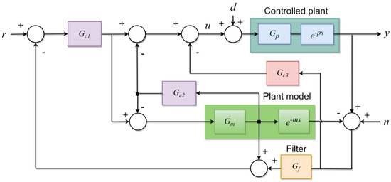
Figure 1.
Modified Smith predictor structure proposed by Ajmeri and Ali [18] (reproduced with permission from Ajmeri and Ali). Analytical design of a modified Smith predictor for unstable second-order processes with time delay, published by International Journal of Systems Science, 2017.
Equations (1) and (2) are obtained with the superposition principle under normal conditions (Gm = Gp, e−ms= e−ps) for input reference (r) and input disturbance (d) when the system parameters and time delay values are known exactly and do not change. The closed-loop transfer function between the plant output (y) and the input reference (r) is:
In Equation (1), e−θs= e−ps = e−ms. As can be seen from Equation (1), which is derived from normal situations, the performance of set-point tracking depends on the performance of the Gc1 and Gc2 controllers, but it does not depend on Gc3. Again, it is seen that the 1 + (Gc1 + Gc2)Gm = 0 characteristic equation of Equation (1) does not depend on the plant time delay. Thus, the Gc1 and Gc2 controllers can be designed independently of the time delay. The closed-loop transfer function between the plant output (y) and the disturbance (d) is:
when Equation (2), obtained for normal situations, is examined, it can be seen that the disturbance rejection performance depends on all the Gc1, Gc2, and Gc3 controllers, as well as on the time delay.
In this study, because the set-point tracking performance depends only on the Gc1 and Gc2 controllers, the design procedure for the controllers was first carried out for the Gc1 and Gc2 controllers and then for the Gc3 controller on the disturbance rejection side. The design procedure was carried out using the direct synthesis approach suggested by Rao and Chidambaram [15], Uma and Rao [16], and Ajmeri and Ali [18]. In addition, the method proposed in this study was compared with the aforementioned studies.
2.2. Design of Controllers
There were three types of SOUPTD models used in the paper. The first plant model has two unstable poles, the second has one unstable pole and one pole at the origin, and the third has one stable and one unstable pole. The second plant model can be approximated to the first plant model by assuming a parameter (γ), as shown in Equation (4) [18]. The plant models used are presented in Equations (3)–(5).
The explanation of the analytical method proposed in the study, for the design of the controllers in the SP structure, is made on the SOUPTD model shown in Equation (6), which has two roots in the right half plane of the complex plane. In Equation (6), Gm represents the model of the plant, K is the plant gain, T1 and T2 are the time constants, and θ is the time delay.
2.2.1. Direct Synthesis Approach of Gc1 and Gc2 Controllers
In the SP structure, the I-PD controller structure on the set-point tracker side and the PD controller structure on the disturbance rejection side are proposed. The transfer functions of the Gc1 and Gc2 controllers are provided in Equations (7) and (8), respectively:
and substituting Equations (7) and (8) in Equation (1) obtains Equation (9):
The direct synthesis approach relies on changing a single design or tuning parameter to strike a balance between system performance and robustness [18]. Here, for the design of the controllers, a reference model is first defined to achieve the desired closed-loop performance and robustness. The numerator and denominator parts of the plant model, designed using the reference model, are equalized, and the searched parameters are found. The reference model used in the design is given in Equation (10):
In Equation (10), λ is the tuning parameter. If the denominator parts of Equation (9) and Equation (10) are equalized, the controller parameters given in Equations (11)–(13) are obtained. Here, it is obvious that ϕ =K. According to Equations (11)–(13), the parameters of set-point tracker controllers can be easily tuned using the λ parameter, taking into account the set-point performance and robustness status. θ, which expresses the plant time delay, is used for the selection of the λ parameter [15,16,18]. The numerical example for the selection of λ is shown in Example 1.
2.2.2. Design of Gc3 Controller
For the Gc3 controller, a PD controller in cascade with a lead–lag filter is taken, and its transfer function is given in Equation (14):
by substituting Gc3 in Equation (2) and replacing the exponential term with first-order Pade’s approximation for e−θs, Equation (15) is obtained, and if α= θ/2 is chosen for simplicity [18], Equation (16) is obtained:
Here, as in the design of the set-point tracking controller above, a reference model is selected that provides both stability and robustness. The model determined for Equation (16) is shown in Equation (17). Ensuring stability and robustness depends on the choice of the ψ and τ parameters in Equation (17). The τ and ψ parameters are multiplied here. It appears that, as two tuning parameters, stability and robustness can only be tuned with ψ according to a constant chosen value for τ. In our study, the τ value was chosen as τ = θ/2, and ψ was used as the tuning parameter. The reason for taking τ as θ/2 and the consequent determination of ψ is explained in Example 1.
Controller parameters are determined by equalizing the coefficients in Equations (16) and (17). Gc3 controller parameters are formulated in Equations (18)–(20):
The obtained controller parameters are also valid for the Gp2 model given in Equation (4). The controller parameters for the Gp3 model can be obtained by following the same design methodology applied to the Gp1 and Gp2 models. The controller parameters obtained for all models are set out in Table 1 (λ = θ, τ = 0.5θ, ϕ = K are taken for all the plant models in Table 1).

Table 1.
Plant models and controller parameter formulas.
3. Results
The contribution of the suggested design method is presented in simulation studies for second-order plus time-delay plant samples. The first plant model has two unstable poles, the second has one stable and one unstable pole, and the third has one unstable pole and one pole at the origin. The plant models used are presented in Equations (21)–(23).
The IAE index given in Equation (24) was used to compare the performances of the controllers. Here, e is the difference between the reference and the plant output.
3.1. Example 1
As seen in this plant example, K = 2, θ = 0.3, T1 = 3, and T2 = 1. In this example, we first explain the determination of τ and the identification of ψ according to the found τ value. Considering Equation (18), this is defined as dependent on τ such that ψ is greater than 1. This definition is given in Equation (25):
The load disturbance was investigated by taking 1.5θ, θ, and 0.5θ of τ. The load disturbance rejection response, according to these three values of θ, is shown in Figure 2.
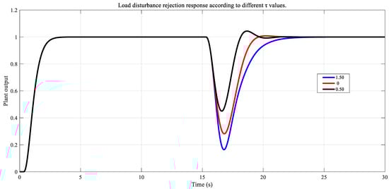
Figure 2.
Load disturbance rejection response according to different τ values.
According to Figure 2, it can be seen that the most appropriate system response to eliminate the load disturbance is for τ = θ/2, but there is some overshoot. It is necessary to adjust ψ to get a better result by removing the overshoot. System responses for different ψ values were obtained and are presented in Figure 3. According to these results, ψ = 1.12 was determined.
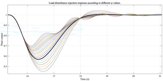
Figure 3.
Load disturbance rejection response according to different ψ values.
The process for the determination of τ and ψ, presented here, has been applied in other examples, which are not shown here. By substituting plant values of K = 2, θ = 0.3, T1 = 3, and T2 = 1 in Table 1, the controller parameters shown in Table 2 were obtained.
Table 2.
Controller parameters obtained using the method proposed in Example 1.
For the G1(s) plant model, Rao and Chidambaram [15] obtained the controller parameters Kc1 = 4.531, Ki1 = 2.93, Kc2 = 2, Kd2 = 7.62, Kc3 = 2.55, Ki3 = 1.42, Kd3 = 4.481, α = 0.15, and β = 0.0059 for this plant model. Uma and Rao [16] reported that they determined the following controller parameters in their study: Kcs = 8.2274, Kis = 5.5945, Kds = 7.0624, βs = 0.0863, Kcd = 6.6166, Kid = 5.2716, Kdd = 5.8249, αd = 0.15, and βd = 0.0028. On the other hand, Ajmeri and Ali [18] produced a design based on the values of λ = θ and τ = 1.3θ. They obtained Kc1 = 12.7906, Ti1 = 1.013, αc = 7.912, βc = 0.0682, Kc2 = 4.1826, Ti2 = 1.5274, Td2 = 1.2206, α = 0.15, and β = 0.0042 values.
A comparison of the performances of the proposed method and the other methods was performed by applying a unit step reference input at t = 0 and an input step disturbance signal of −2 amplitude at t = 15. The plant output (y) and control signals (u) obtained for this case are presented in Figure 4 and Figure 5.
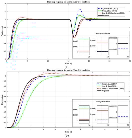
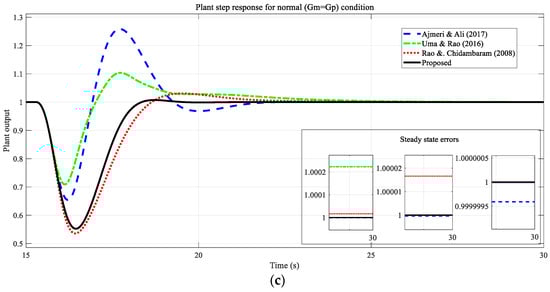
Figure 4.
Closed loop performances of the proposed method and other methods for Example 1. (a) Set-point tracking and disturbance rejection, (b) magnified set-point tracking, and (c) magnified disturbance rejection [15,16,18].
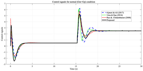
Figure 5.
Control signals of the proposed method and other methods for Example 1 [15,16,18].
As can be seen from Figure 4, the controllers designed using the proposed method have significant performance advantages over the other methods in terms of both set-point tracking and disturbance rejection. The proposed method can capture the reference value in the shortest rise time and without overshooting. The disturbance can also suppress the reference in a short time without overshooting and without oscillation. In addition, as can be seen from the magnified indicators in Figure 4c, superiority was achieved over other methods in terms of steady-state error.
Figure 5 shows control signals applied to the plant. Here, it can be seen that the control signals of the controllers designed using the proposed method overlap with those designed using other methods. The result shows that a better control performance can be obtained for the same, or almost the same, control effort.
The proposed method was compared with the other methods in terms of parameter changes and time-delay changes. For this comparison, the time delay and process gain were increased by 10%, and each time constant was reduced by 5% [18]. Figure 6 presents graphs showing this comparison. The method proposed by Uma and Rao [16] produced unstable output for parameter values in these values, and for this reason, it is not shown in Figure 6. The result of the comparison indicates that the plant output designed using the proposed method is less affected by parameter changes in both reference tracking and load disturbance situations. This shows that the designed system is more robust.
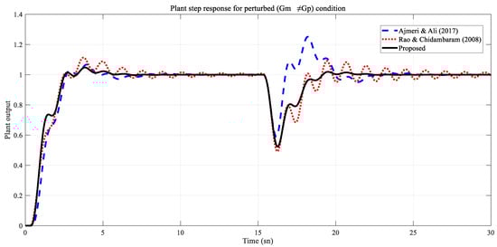
Figure 6.
Performance comparison of the proposed method and other methods, in terms of parameter changes, for Example 1 [15,18].
To show the contribution of the proposed method, the closed-loop IAE performance measure for the exact system model and modified system models is presented in Table 3 for reference tracking and disturbance conditions. As can be seen, the lowest IAE value could be obtained using the proposed method in all cases.
Table 3.
IAE performance measures for Example 1.
Noise is another issue to consider in process control applications. In processes, high-frequency signals in the feedback, due to the internal dynamics of the measuring elements or various electromagnetic effects, are characterized as noise. In many studies, additive Gaussian white noise (AWGN) has been used to simulate sensor noise [46,47,48,49,50]. The proposed method was also compared, in terms of measurement noise, with the methods of Ajmeri and Ali (2017), which are closest to the proposed method in terms of performance. For this purpose, two tests were carried out by adding white Gaussian noise to the system feedback in Figure 1. The used noise test signals are presented in Figure 7. Both test signals have a zero mean. The standard deviation of Signal 1 is 0.01 and the standard deviation of Signal 2 is 0.1. In noise tests, a low-pass filter is connected, in series, with the derivative operator in the controller on the load disturbance rejection side (Gc3) in the suggested method to keep the effect of noise to a minimum. The low-pass filter time constant (Tf) equals 0.05Td3. Test results for Example 1 are presented in Figure 8. Noise tests show both methods are affected by the noise situation. Although both methods can maintain their stability, it is seen that the plant output of the proposed method is less vibratory than the other method.
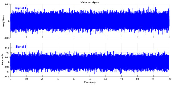
Figure 7.
Noise test signals.
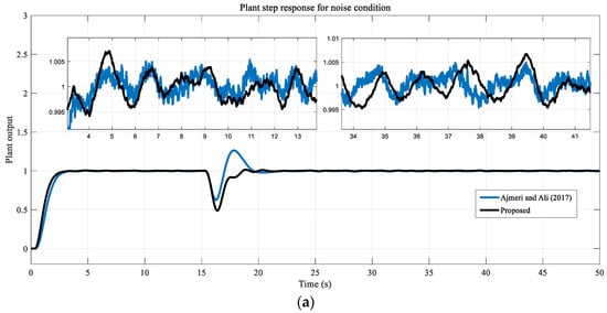
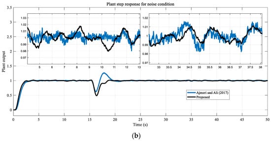
Figure 8.
Performance comparison of the proposed method, in terms of noise effects, for Example 1. (a) Test result for noise Signal 1 and (b) test result for noise Signal 2 [18].
3.2. Example 2
The parameters of the second plant sample were K = 1, θ = 1.2, T1 = 1, and T2 = 0.5. The controller parameters were obtained using our suggested method. Ajmeri and Ali [18] compared their proposed method for this plant model with the studies of Rao and Chidambaram [15] and Uma and Rao [16]. The controller parameters obtained by Ajmeri and Ali [18] using the two methods mentioned above, as well as those obtained using our suggested method, are shown in Table 4.
Table 4.
Controller parameters for Example 2.
As in the previous example, the proposed methods were compared in terms of set-point tracking, disturbance input, and parameter changes. The results obtained are presented in Figure 9.
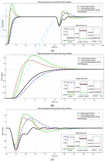
Figure 9.
Closed loop performances of the proposed method and other methods for Example 2. (a) Set-point tracking and disturbance rejection, (b) magnified set-point tracking, and (c) magnified disturbance rejection [15,16,18].
In the Figure 9b, it can be seen that the proposed method and Ajmeri and Ali’s [18] methods reach the reference value with no overshooting at approximately the same rise time. In this section, it can, again, be seen that the methods of Rao and Chidambaram [15] and Uma and Rao [16] are fast but exhibit very high overshoot rates. An input step disturbance value of −0.05 was applied to the system at t = 50, and the result obtained is shown in Figure 9c. It can be seen that the method proposed in our study can eliminate the disturbance input in the shortest time with negligible overshoot but with a little oscillation, whereas other methods can overcome this process with high overshooting and settling time. In terms of steady-state error, the method of Rao and Chidambaram [15] was shown to have the lowest value, and the proposed method is very close to this value, whereas the other methods exhibit a larger steady-state error.
Control signals for the proposed method and the other methods are presented in Figure 10. As can be seen, an effort close to the control signal of Ajmeri and Ali [18] is applied on the set-point tracking side, and a higher control effort is exhibited in the methods of Rao and Chidambaram [15] and Uma and Rao [16]. On the disturbance rejection side, the lowest control effort is found in our recommended method. This result shows that the best control performance with low effort is obtained using the proposed method.
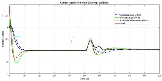
Figure 10.
Control signals of the proposed method and other methods for Example 2 [15,16,18].
Figure 11 presents the results obtained for the robustness test. In the robustness test, the only change was to increase the system time delay by 5%. As can be seen, the most robust control performance was obtained using the proposed method. The IAE performance criteria for the normal state and parameter variations are given in Table 5. The same noise test as in the previous example was also performed for this example, and the results are given in Figure 12.
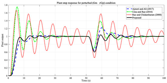
Figure 11.
Performance comparison of the proposed methods and other methods, in terms of parameter changes, for Example 2 [15,16,18].
Table 5.
IAE performance measures for Example 2.
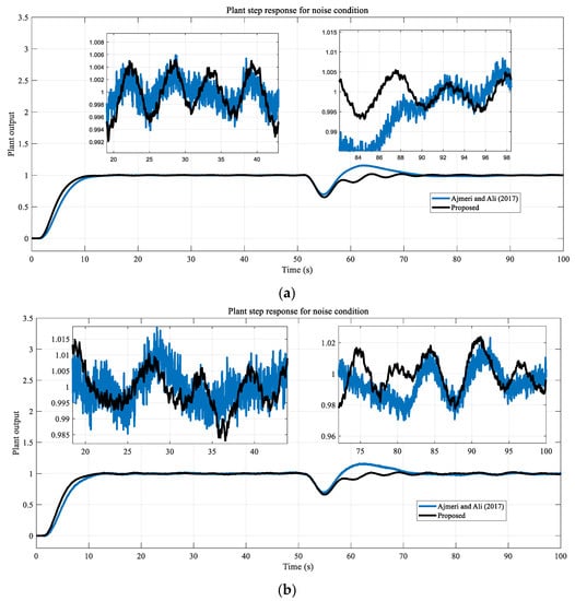
Figure 12.
Performance comparison of the proposed method, in terms of noise effects, for Example 2. (a) Test result for noise Signal 1 and (b) test result for noise Signal 2 [18].
3.3. Example 3
The controller parameters for this example are provided in Table 6. Here, comparisons are based on tests similar to those used in the two previous examples. An input step disturbance with an amplitude of −1 was applied to the system at 15 s. Plant parameters and time delay were increased by 20%. In this case, the perturbed model shown in Equation (26) was obtained as a result of the parameter change, and this model was used for the robustness comparison.
Table 6.
Controller parameters for Example 3.
The test results obtained for normal situations are shown in Figure 13. In this test, the shortest rise time, the shortest settling time, and the lowest overshoot were obtained with the proposed method (Figure 13b). The recommended method was able to suppress the disturbance entry in the 15th second, with the lowest overshoot rate, least oscillation, and the shortest settling time (Figure 13c). When the steady-state error is examined, it can be concluded that the method of Ajmeri and Ali (2017) and the proposed method are very close to each other and at the lowest rate.
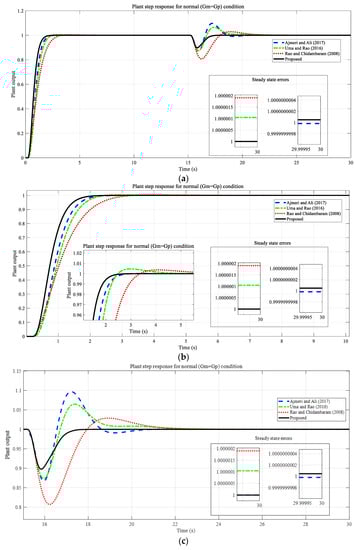
Figure 13.
Closed loop performances of the proposed method and other methods for Example 3. (a) Set-point tracking and disturbance rejection, (b) magnified set-point tracking, and (c) magnified disturbance rejection [15,16,18].
The control signals are presented in Figure 14. The control effort by set-point tracking of the proposed method is slightly larger than that of other methods, but the difference is small. On the disturbance rejection side, it is at almost the same level as the other methods. The IAE performance criteria for the normal state and parameter variations are given in Table 7.
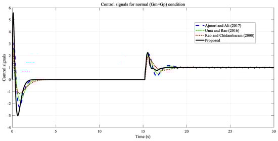
Figure 14.
Control signals of the proposed method and other methods for Example 3 [15,16,18].
Table 7.
IAE performance measures for Example 3.
From the results shown in Figure 15, it can be seen that the proposed method maintains its robustness with parameter changes. The overshoot rate and oscillations increased in the methods of Ajmeri and Ali [18] and Uma and Rao [16]. In the method proposed by Rao and Chidambaram [15], some decrease in overshoot and a slight increase in settling time occurs. In our proposed method, the overshoot rate and oscillation increased slightly. Noise test results are presented in Figure 16.
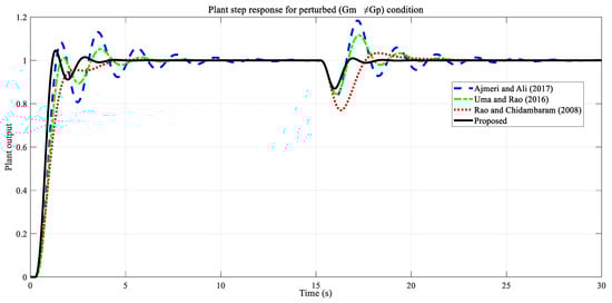
Figure 15.
Performance comparison of the proposed method and the other methods, in terms of parameter changes, for Example 3 [15,16,18].
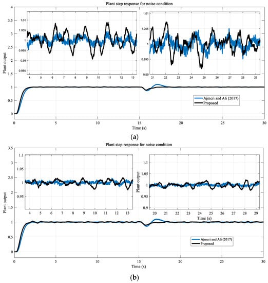
Figure 16.
Performance comparison of the proposed method, in terms of noise effects, for Example 3. (a) Test result for noise Signal 1, (b) test result for noise Signal 2 [18].
4. Conclusions
In this article, we have discussed a design method based on the direct synthesis approach on the modified Smith predictor structure presented by Ajmeri and Ali. In contrast with other studies, the I-PD controller structure was used on the set-point tracker side of the Smith predictor, and a cascade PD lead–lag controller was used on the disturbance rejection side. By choosing I-PD and PD lead–lag controllers, the number of controller parameters that need to be calculated are reduced, and the mathematical expressions that emerge in this direct synthesis approach are significantly reduced. The proposed method was studied under the load disturbance for normal and perturbed states on three unstable second-order plus time-delay system models. The first plant model had two unstable poles, the second had one stable and one unstable pole, and the third had one unstable pole and one pole at the origin. When the results obtained using the proposed method are compared with results obtained using other methods set out in the literature, significant improvements have been achieved in terms of the set-point tracking, disturbance rejection, and robustness conditions.
Author Contributions
Writing–original draft preparation, Y.İ. and M.S.C.; simulations, M.S.C.; editing, Y.İ. All authors have read and agreed to the published version of the manuscript.
Funding
This research received no external funding.
Institutional Review Board Statement
Not applicable.
Informed Consent Statement
Not applicable.
Data Availability Statement
Where no new data were created.
Conflicts of Interest
The authors declare no conflict of interest.
References
- Korupu, V.L.; Muthukumarasamy, M. A comparative study of various Smith predictor configurations for industrial delay processes. Chem. Prod. Process Model. 2021, 17, 701–732. [Google Scholar] [CrossRef]
- Laifa, S.; Boudjehem, B.; Gasmi, H. Direct synthesis approach to design fractional PID controller for SISO and MIMO systems based on Smith predictor structure applied for time-delay non integer-order models. Int. J. Dynam. Control 2021, 10, 760–770. [Google Scholar]
- Kaya, I. A PI-PD controller design for control of unstable and integrating processes. ISA Trans. 2003, 42, 111–121. [Google Scholar] [CrossRef] [PubMed]
- Kaya, I. PI-PD controllers for controlling stable processes with inverse response and dead time. Electr. Eng. 2015, 98, 55–65. [Google Scholar] [CrossRef]
- Zheng, M.; Huang, T.; Zhang, G. A New Design Method for PI-PD Control of Unstable Fractional-Order System with Time Delay. Complexity 2019, 2019. [Google Scholar] [CrossRef]
- Alyoussef, F.; Kaya, I. Simple PI-PD tuning rules based on the centroid of the stability region for controlling unstable and integrating processes. ISA Trans. 2023, 134, 238–255. [Google Scholar] [CrossRef]
- Normey-Rico, J.E.; Camacho, E.F. A Predictor-based Solution: The Smith Predictor. In Control of Dead-Time Processes; Advanced Textbooks in Control and Signal Processing series; Springer: London, UK, 2007; pp. 48–51. [Google Scholar]
- Henry, T.; Cao, Y. Modified smith predictor for slug control with large valve stroke time in unstable systems. Digit. Chem. Eng. 2022, 3. [Google Scholar] [CrossRef]
- Palmor, Z.J.; Powers, D.V. Improved dead-time compensator controllers. AIChE J. 1985, 31, 215–221. [Google Scholar] [CrossRef]
- Huang, H.P.; Chen, C.-L.; Chao, Y.-C.; Chen, P.-L. A modified smith predictor with an approximate inverse of dead time. AIChE J. 1990, 36, 1025–1031. [Google Scholar] [CrossRef]
- Majhi, S.; Atherton, D.P. A new Smith predictor and controller for unstable and integrating processes with time delay. In Proceedings of the 37th IEEE Conference on Decision & Control, Tampa, FL, USA, 18 December 1998. [Google Scholar]
- Zhang, W.; Sun, Y.; Xu, X. Two degree-of-freedom smith predictor for processes with time delay. Automatica 1998, 34, 1279–1282. [Google Scholar] [CrossRef]
- Kaya, I. A new Smith predictor and controller for control of processes with long dead time. ISA Trans. 2003, 42, 101–110. [Google Scholar] [CrossRef]
- Kaya, I. Auto tuning of a new PI-PID Smith predictor based on time domain specifications. ISA Trans. 2003, 42, 559–575. [Google Scholar] [CrossRef]
- Rao, A.S.; Chidambaram, M. Analytical design of modified Smith predictor in a two-degrees-of-freedom control scheme for second order unstable processes with time delay. ISA Trans. 2008, 47, 407–419. [Google Scholar] [CrossRef] [PubMed]
- Uma, S.; Rao, A.S. Enhanced modified Smith predictor for second order non-minimum phase unstable processes. Int. J. Syst. Sci. 2016, 47, 966–981. [Google Scholar] [CrossRef]
- Özbek, N.S.; Eker, I. A fractional fuzzy PI-PD based modified Smith predictor for controlling of FOPDT process. In Proceedings of the 5th International Conference on Electronic Devices Systems and Applications (ICEDSA), Ras Al Khaimah, United Arab Emirates, 6–8 December 2016; pp. 1–4. [Google Scholar]
- Ajmeri, M.; Ali, A. Analytical design of modified Smith predictor for unstable second-order processes with time delay. Int. J. Syst. Sci. 2017, 48, 1671–1681. [Google Scholar] [CrossRef]
- Sanz, R.; García, P.; Albertos, P. A generalized smith predictor for unstable time-delay SISO systems. ISA Trans. 2018, 72, 197–204. [Google Scholar] [CrossRef]
- Espín, J.; Castrillon, F.; Leiva, H.; Camacho, O. A modified Smith predictor based–Sliding mode control approach for integrating processes with dead time. Alex. Eng. J. 2022, 61, 10119–10137. [Google Scholar] [CrossRef]
- Mejía, C.; Salazar, E.; Camacho, O. A comparative experimental evaluation of various Smith predictor approaches for a thermal process with large dead time. Alex. Eng. J. 2022, 61, 9377–9394. [Google Scholar] [CrossRef]
- Li, S.; Li, J. Output Predictor-Based Active Disturbance Rejection Control for a Wind Energy Conversion System with PMSG. IEEE Access 2017, 5, 5205–5214. [Google Scholar] [CrossRef]
- Liu, T.; Hao, S.; Li, D.; Chen, W.-H.; Wang, Q.-G. Predictor-Based Disturbance Rejection Control for Sampled Systems with Input Delay. IEEE Trans. Control Syst. Technol. 2019, 27, 772–780. [Google Scholar] [CrossRef]
- Bowthorpe, M.; Tavakoli, M.; Becher, H.; Howe, R. Smith Predictor-Based Robot Control for Ultrasound-Guided Teleoperated Beating-Heart Surgery. IEEE J. Biomed. Health Inform. 2014, 18, 157–166. [Google Scholar] [CrossRef] [PubMed]
- Fu, C.; Tan, W. Linear Active Disturbance Rejection Control for Processes with Time Delays: IMC Interpretation. IEEE Access 2020, 8, 16606–16617. [Google Scholar] [CrossRef]
- Feng, Z.; Peña-Alzola, R.; Syed, M.H.; Norman, P.J.; Burt, G.M. Adaptive Smith Predictor for Enhanced Stability of Power Hardware-in-The-Loop Setups. IEEE Trans. Ind. Electron. 2020, 1–10. [Google Scholar] [CrossRef]
- Ghorbani, M.; Tavakoli-Kakhki, M.; Tepljakov, A.; Petlenkov, E. Robust stability analysis of smith predictor based interval fractional-order control systems: A case study in level control process. IEEE/CAA J. Autom. Sin. 2023, 10, 762–780. [Google Scholar] [CrossRef]
- Luo, Y.; Xue, W.; He, W.; Nie, K.; Mao, Y.; Guerrero, J.M. Delay-Compound-Compensation Control for Photoelectric Tracking System Based on Improved Smith Predictor Scheme. IEEE Photonics J. 2022, 14, 1–8. [Google Scholar] [CrossRef]
- Grelewicz, P.; Nowak, P.; Czeczot, J.; Musial, J. Increment Count Method and Its PLC-Based Implementation for Autotuning of Reduced-Order ADRC with Smith Predictor. IEEE Trans. Ind. Electron. 2021, 68, 12554–12564. [Google Scholar] [CrossRef]
- Ren, W.; Luo, Y.; He, Q.N.; Zhou, X.; Deng, C.; Mao, Y.; Ren, G. Stabilization Control of Electro-Optical Tracking System with Fiber-Optic Gyroscope Based on Modified Smith Predictor Control Scheme. IEEE Sens. J. 2018, 18, 8172–8178. [Google Scholar] [CrossRef]
- Bolignari, M.; Rizzello, G.; Zaccarian, L.; Fontana, M. Smith-Predictor-Based Torque Control of a Rolling Diaphragm Hydrostatic Transmission. IEEE Robot. Autom. Lett. 2021, 6, 2970–2977. [Google Scholar] [CrossRef]
- Sakthivel, R.; Mohanapriya, S.; Almakhles, D.J. Robust Tracking and Disturbance Rejection Performance for Vehicle Dynamics. IEEE Access 2019, 7, 118598–118607. [Google Scholar] [CrossRef]
- Liu, P.; Song, Y.; Yan, P.; Sun, Y. Actuator Saturation Compensation for Fast Tool Servo Systems with Time Delays. IEEE Access 2021, 9, 6633–6641. [Google Scholar] [CrossRef]
- Zhou, X.; Zhou, J.; Yang, C.; Gui, W. Set-Point Tracking and Multi-Objective Optimization-Based PID Control for the Goethite Process. IEEE Access 2018, 6, 36683–36698. [Google Scholar] [CrossRef]
- Wai, R.-J.; Lee, J.-D.; Chuang, K.-L. Real-Time PID Control Strategy for Maglev Transportation System via Particle Swarm Optimization. IEEE Trans. Ind. Electron. 2011, 58, 629–646. [Google Scholar] [CrossRef]
- Tran, V.P.; Santoso, F.; Garratt, M.A. Adaptive Trajectory Tracking for Quadrotor Systems in Unknown Wind Environments Using Particle Swarm Optimization-Based Strictly Negative Imaginary Controllers. IEEE Trans. Aerosp. Electron. Syst. 2021, 57, 1742–1752. [Google Scholar] [CrossRef]
- Behera, A.; Panigrahi, T.K.; Ray, P.K.; Sahoo, A.K. A novel cascaded PID controller for automatic generation control analysis with renewable sources. IEEE/CAA J. Autom. Sin. 2019, 6, 1438–1451. [Google Scholar] [CrossRef]
- Zahid, T.; Kausar, Z.; Shah, M.F.; Saeed, M.T.; Pan, J. An Intelligent Hybrid Control to Enhance Applicability of Mobile Robots in Cluttered Environments. IEEE Access 2021, 9, 50151–50162. [Google Scholar] [CrossRef]
- Safaei, M.; Tavakoli, S. Smith predictor based fractional-order control design for time-delay integer-order systems. Int. J. Dyn. Control 2018, 6, 179–187. [Google Scholar] [CrossRef]
- Kaya, I. I-PD Controller Design for Integrating Time Delay Processes Based on Optimum Analytical Formulas. IFAC-PapersOnLine 2018, 51, 575–580. [Google Scholar] [CrossRef]
- Chakraborty, S.; Ghosh, S.; Naskar, A.K. I-PD controller for integrating plus time delay processes. IET Control Theory Appl. 2017, 11, 3137–3145. [Google Scholar] [CrossRef]
- Kaya, I.; Peker, F. Optimal I-PD controller design for setpoint tracking of integrating processes with time delay. IET Control Theory Appl. 2020, 14, 2814–2824. [Google Scholar] [CrossRef]
- Peker, F.; Kaya, I. Maximum sensitivity (Ms)-based I-PD controller design for the control of integrating processes with time delay. Int. J. Syst. Sci. 2023, 54, 313–332. [Google Scholar] [CrossRef]
- Dogruer, T. Design of I-PD Controller Based Modified Smith Predictor for Processes with Inverse Response and Time Delay Using Equilibrium Optimizer. IEEE Access 2023, 11, 14636–14646. [Google Scholar] [CrossRef]
- Normey-Rico, J.E.; Camacho, E.F. Improving the robustness of dead time compensating PI controllers. Control Eng. Pract. 1997, 5, 801–810. [Google Scholar] [CrossRef]
- So, G.B. Design of an Intelligent NPID Controller Based on Genetic Algorithm for Disturbance Rejection in Single Integrating Process with Time Delay. J. Mar. Sci. Eng. 2021, 9, 25. [Google Scholar] [CrossRef]
- Ding, L.; Wang, H.N.; Guan, Z.H.; Chen, J. Tracking Under Additive White Gaussian Noise Effect. In Proceedings of the 7th Asian Control Conference, Hong Kong, China, 27–29 August 2009. [Google Scholar]
- Garcia, J.D.G. Design and performance assessment criteria for controllers applied to Magnetic Bearings. In Proceedings of the Electrodynamic and Mechatronic Systems (SCE III), Opole, Poland, 6–8 October 2011; pp. 17–22. [Google Scholar]
- Devi, R.; Dewan, L. Effect of different noises on PID controller performance and their comparative denoising using wavelets. In Proceedings of the 2017 8th International Conference on Computing, Communication and Networking Technologies (ICCCNT), Delhi, India, 3–5 July 2017; pp. 1–6. [Google Scholar]
- Chi, M.; Guan, Z.-H.; Ding, L.; Yuan, F.-S. Tracking performance under additive Gaussian Noise and control energy constraint for networked control systems. In Proceedings of the 2012 24th Chinese Control and Decision Conference (CCDC), Taiyuan, China, 23–25 May 2012; pp. 518–522. [Google Scholar]
Disclaimer/Publisher’s Note: The statements, opinions and data contained in all publications are solely those of the individual author(s) and contributor(s) and not of MDPI and/or the editor(s). MDPI and/or the editor(s) disclaim responsibility for any injury to people or property resulting from any ideas, methods, instructions or products referred to in the content. |
© 2023 by the authors. Licensee MDPI, Basel, Switzerland. This article is an open access article distributed under the terms and conditions of the Creative Commons Attribution (CC BY) license (https://creativecommons.org/licenses/by/4.0/).