Abstract
This paper introduces and studies a new discrete distribution with one parameter that expands the Poisson model, discrete weighted Poisson Lerch transcendental (DWPLT) distribution. Its mathematical and statistical structure showed that some of the basic characteristics and features of the DWPLT model include probability mass function, the hazard rate function for single and double components, moments with auxiliary statistical measures (expectation, variance, index of dispersion, skewness, kurtosis, negative moments), conditional expectation, Lorenz function, and order statistics, which were derived as closed forms. DWPLT distribution can be used as a flexible statistical approach to analyze and discuss real asymmetric leptokurtic data. Moreover, it could be applied to a hyperdispersive data model. Two different estimation methods were derived, i.e., maximal likelihood and the moments technique for the DWPLT parameter, and some advanced numerical methods were utilized for the estimation process. A simulation was performed to examine and analyze the performance of the DWPLT estimator on the basis of the criteria of the bias and mean squared errors. The flexibility and fit ability of the proposed distribution is demonstrated via the clinical application of a real dataset. The DWPLT model was more flexible and worked well for modeling real age data when compared to other competitive age distributions in the statistical literature.
1. Introduction
In life testing and reliability analysis situations, it is often difficult to measure the life of a device or component on a continuous scale. For example, in survival analysis, the number of days that a patient survived after treatment or of recorded hours/days representing the time from remission to relapse is a random discrete variable. Similarly, in reliability experiments, the life of a device receiving a number of shocks before failure or of an on/off switching machine whose longevity depends on the number of times the device is turned on/off is discrete. In all these cases, lifetime and age cannot be measured on a continuous scale but are simply computed, so discrete distributions are better options for modeling therm.
In the past few decades, many papers focusing on discrete distributions have been presented for modeling lifetime data in many fields, such as insurance, engineering, agriculture, and the medical, physical, and biological sciences. A continuous random variable may be characterized by, for example, its cumulative distribution function, probability density function, moments, hazard rate functions, and reversed hazard rate functions. The discrete analog of the continuous model is mainly constructed on the basis of the principle of preserving one or more characteristic properties of the continuous characteristic. Thus, there are various techniques of discretizing a continuous model depending on the property we want to preserve.
In stress-force models and analysis, the system or component encounters random stress during its function and has an inherent variable force that allows for it to work only when the force is greater than the stress. Its chance of success is called reliability. If the force and stress distributions are known, reliability can usually be obtained using normal transformation techniques. However, when the functional relationships of force and tension are complex, such analytical techniques are intractable. In this case, the exact solution is not available, and an alternative technique must be adopted to roughly approximate the actual reliability, for example, (i) Monte Carlo simulation approaches, (ii) Taylor series methods, (iii) numerical integration techniques, and (iv) discretization techniques. For more details, see Yari and Tondpour [1]. Here, a discretization approach was applied to create a flexible discrete probabilistic model with one parameter. Because of the flexibility of the discretization approach, it has been used by many authors in the statistical literature to produce adaptive discrete models; for instance, discrete Rayleigh distribution by Roy [2], discrete Burr and discrete Pareto distributions by Krishna and Pundir [3], the generalization of geometric distribution by Gomez-Déniz [4], discrete inverse Weibull distribution by Jazi et al. [5], discrete Burr Type III distribution by Al-Huniti and Al-Dayian [6], the discrete generalized exponential distribution of the second type by Nekoukhou et al. [7], discrete inverse Rayleigh distribution by Hussain and Ahmad [8], two-parameter discrete Lindley distribution by Hussain et al. [9], discrete Lindley distribution by Abebe and Shanker [10], new discrete Lindley distribution by Al-Babtain et al. [11], new three-parameter discrete Lindley distribution by Eliwa et al. [12], and new extended geometric distribution by Almazah et al. [13].
This study focuses on an extension of Poisson distribution. The Poisson model is used extensively for modeling count data in a range of different scientific fields. For this reason, many researchers have studied its properties, extensions, and modifications, and proposed generalizations to modify and increase the initial distribution proposed by Poisson [14]. Although the mean of a Poisson distribution equalling its variance is useful in specific situations, this often limits the ability of the distribution to accurately model practical data. To weaken this assumption and overcome the limitations of Poisson distribution, several authors have developed different discrete distributions for modeling asymmetrically dispersed count data. Castillo and Pérez-Casany [15] proposed a weighted Poisson distribution for over- and underdispersion situations from the concept of the weighted distribution introduced by Fisher [16] in conjunction with Poisson distribution. The weighted Poisson distribution overcomes the inherent limitation of scattering equivalence and can model multimodal data. Another valuable property of this distribution is its ability to model and describe truncated data (see Dietz and Bhning [17]). Moreover, several general properties of the weighted Poisson distribution were examined by Kokonendji et al. [18], who expanded on the paper published by Castillo and Perez-Casany [15], and specifically on how the shape of the weight function relates to the dispersion of the resulting weighted Poisson distribution.
Given the significance of weighted Poisson distribution, a new elastic extension was established in the discrete weighted Poisson–Lerch transcendent (DWPLT) model, which is weighted Poisson distribution from the discrete Burr–Hatke model (see El-Morshedy et al. [19]). Thus, the resulting model is DWPLT distribution. The cumulative distribution function (CDF) of the DWPLT model can be expressed as follows:
where x is any value belonging to the positive domain of discrete random variable X, is a scale parameter of the DWPLT model, and is the Lerch transcendent function that can be computed with HurwitzLerchPhi in Mathematica software (see Wolfram Research [20]). The corresponding probability mass function (PMF) to Equation (1) is as follows:
Equation (2) can be derived via a survival discretization approach as follows:
where . It is easy to show that ; then, the PMF is the decreasing function in x.If random variables and are independent and have the DWPLT model, PMF for and can be formulated as follows, respectively:
and
where ,
In medical and engineering fields, the distribution of two random variables and is very important. In engineering, random variable Y or Z can be referred to as the sum of two signals from two different sources or the sum of stresses from two sources on a component/machine. In medicine, random variable Y or Z can be, for example, the effect of two diseases on a specific organ in the human body. Assuming that random variable X had DWPLT distribution, the hazard rate function (HRF) is as follows:
where . Figure 1 shows the PMF and HRF plots for different values of the DWPLT parameter.
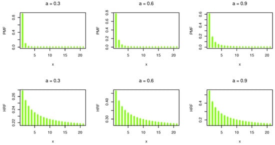
Figure 1.
PMF and HRF plots.
The shape of the PMF and HRF always decreases. Moreover, PMF can be applied to discuss and evaluate asymmetric unimodal data. Suppose that and are independent DWPLT variables with parameters and , respectively. Then, the HRF of is given as follows:
where Since the PMF of X decreased in x, X had decreasing reversed HRF (DRHRF). Let F be the DWPLT life distribution, and the corresponding PMF be denoted by sequence . Then, this sequence has DRHRF.
2. Statistical Properties
2.1. Moments and Auxiliary Statistical Measures
Descriptive statistics is an invaluable tool used in data analysis, as it allows for summarizing and interpreting large datasets, providing a concise overview of the key points. Descriptive statistics provide quantifiable information about the data such as the mean, median, variance, standard deviation, skewness, and kurtosis range that can be presented in graphical form. This enables us to quickly identify patterns and trends within the data, allowing for more accurate conclusions to be drawn. Additionally, descriptive statistics can be used to identify outliers in the data, thus providing an even more comprehensive understanding of the dataset. Assuming that random variable X had the DWPLT model, the probability generating function (PrGF) could be expressed as follows:
The corresponding moment generating function (MGF) to Equation (6) is as follows:
The first four moments of X are as follows:
For the moments, symbolic software such as Maple was used. On the basis of the PMF and the law of mathematical expectation, the moments were derived in closed forms. Variance, skewness, and kurtosis can also be derived in closed forms: , , and . Figure 2 shows descriptive statistics of the proposed model on the basis of various values of the distribution parameter.
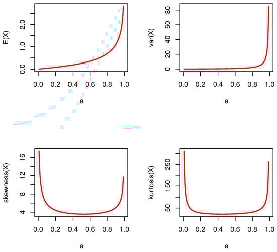
Figure 2.
Descriptive statistics of DWPLT distribution.
The expectation value was less than the value of the variance for all parameter spaces/domains. Thus, the proposed distribution could be used to model overdispersed data. This important feature can be applied to discuss and evaluate actual data. Moreover, it can be used as a flexible probability model for analyzing positively skewed leptokurtic data. The first-order negative moment (NeM) for any and is as follows:
In general, the theory behind the existence of negative moments (NeMs) is very difficult and not as complete as that involving positive moments. However, NeMs have many applications, especially in communication networks and the Fourier transforms of function density.
2.2. Conditional Expectation
Conditional distribution is a statistical concept that describes the probability of an event occurring when another event has already occurred. This type of distribution is useful in examining the probability of outcomes that are dependent on a specific event. Conditional distribution is used in a variety of applications, including predictive analytics, forecasting, and decision making. This type of probability is calculated by dividing the probability of the two events occurring together by the probability of the first event occurring alone. Conditional distribution can also be used to analyze the relationship between two variables. This type of analysis can help in understanding how a change occurs. Considering that random variable X had the DWPLT model, the conditional expectations for and are as follows, respectively:
and
Once the value of the model parameter had been calculated, the conditional expectation was reported to the DWPLT model.
2.3. Order Statistic (OrSc)
In statistics, the nth OrSc of a statistical sample is equal to its n-th smallest value. Order statistics (OrSs) and rank statistics are among the most basic approaches to nonparametric statistics and inferences. Important special cases of the OrSs are the minimal and maximal values, median, and other quantiles of a sample. OrSs are the estimation basis for upper- or lower-score data, and all types of censored data (left, right, climatic, interval, random, progressive). Thus, the possibility of using corresponding CDF and PMF for recorded/ordered observations is intriguing, especially in medical and engineering fields. Suppose that , is a random sample from the DWPLT model, and let ,⋯, be their corresponding order statistics. Then, the CDF of the i-th order statistics for an integer value of x is as follows:
where and The PMF of the ith order statistics can be listed as
According to the PMF of the i-th order statistics, some descriptive statistics can be derived on the basis of the L-moment concept.
2.4. Lorenz Curve
Variability in a statistical series can be measured via various scales such as the Lorenz curve (LoC), which is the cumulative percentage curve. Generally, Lorenz curves are applied to measure the variance/variability in the distribution of income and wealth. Hence, the LoC is a measure of deviation in the actual distribution of the statistical series from the line of the isoquant. The extent of this deviation is the Lorenz modulus. If the distance between the LoC and the isoquant curve is greater, there is more inequality or variance in the series and vice versa. Assuming that random variable X had DWPLT distribution, the LoC function of X is defined as follows:
The advantages of the LoC are that it is attractive and gives a rough idea of the extent of dispersion. Further, LoC facilitates comparing two or more series/chains. Its disadvantages are as follows: with the use of the LoC, one can only have a relative idea of the dispersion of a given distribution compared to the isotropy line. Moreover, it does not provide any numerical variance values for the given distribution.
3. Estimation Methods: Unbiased and Consistent Estimators
In this section, two different estimation approaches are derived and discussed in detail: maximal probability and the moment method. The main objective of studying different estimation approaches is to find the best estimator for data analysis to perfect modeling and predictions.
3.1. Maximal Likelihood Estimation
Maximal likelihood estimation (MLE) is a method of estimating unknown parameters by selecting values that maximize the likelihood of observing a given set of data. This technique is often used in various types of statistical modeling such as regression and classification. It is a popular approach due to its simplicity and easy implementation. At its core, MLE is a mathematical approach for finding the probability distribution of an unknown variable on the basis of a given sample of data. This is achieved by finding the maximal value of the likelihood function, which is based on the probability distribution of the given data. The likelihood function is computed by taking the product of the probability of the observations in the dataset. MLE is used in many areas of study, including economics, biology, engineering, and computer science. In economics, it is used for predictions of the probability of future events based on past observations. In biology, it is used to estimate gene frequencies and the relationships between genes. In this section, we determine the MLE of the DWPLT parameter according to a complete sample. was assumed to be a random sample of size n from DWPLT distribution. The log-likelihood function (L) is as follows:
To estimate model parameter a, first partial derivative should be as follows:
Then, the resulting equation equates to zero, namely, it becomes a “normal equation” that cannot be solved analytically.So, an iterative procedure such as Newton–Raphson is required to solve it numerically.
3.2. Moment Estimation
Moment estimation (MoE) is a nonparametric statistical approach utilized to estimate the parameters of a population or a probability model. This technique is often applied when the moments of a probabilistic model/system or model are in closed view. Random variable X had DWPLT distribution. Then, the value of the estimator could be derived via solving the following equation for a:
The estimator of the model could not be expressed in a closed expression. Thus, a digital approach had to be applied.
4. Estimator Performance: Simulation Results
Simulation studies are a popular and effective method of testing estimator performance in a variety of scenarios. By running several simulations, it is possible to approximate real-world performance and gain insight into how well the estimator could function in the field. The first step of a simulation study is to establish the parameters of the experiment. This involves setting up criteria for the data to be sampled, including sample number and size, and the sampling process. Once the parameters are established, the next step is to generate a simulated dataset that matches the specified criteria. This dataset should have features that are as close as possible to the features of real-world data. Once the dataset is generated, the estimator can be applied to the data. Depending on the type of estimator, different metrics may be used to measure the performance of the estimator. These metrics include bias, root mean squared error, and mean absolute error. In this segment, the performance of the MLE and MoE was tested under different schemes for the DWPLT parameter as follows: Scheme I: (∀a = 0.1 |= 20, = 50, = 100, = 150, = 300, = 500, =700, = 1000); Scheme II: (∀a = 0.4 |= 20, = 50, = 100, = 150, = 300, = 500, =700, = 1000); Scheme III: (∀ a = 0.7 |= 20, = 50, = 100, = 150, = 300, = 500, =700, = 1000); Scheme IV: (∀ a = 0.9 |= 20, = 50, = 100, = 150, = 300, = 500, =700, = 1000). Numerical assessments were performed depending on the bias and mean squared errors (MSE). First, we generated samples of the DWPLT model; the results are listed in Table 1 and Table 2, and substantiated in Figure 3 and Figure 4.

Table 1.
Simulation results for DWPLT parameters using the MLE method.
Table 2.
Simulation results for DWPLT parameters using the MoE method.
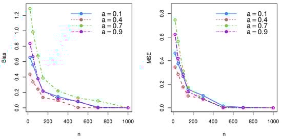
Figure 3.
Simulation results for DWPLT parameters using the MLE method.
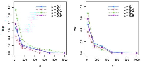
Figure 4.
Simulation results for DWPLT parameters using the MoE method.
According to the simulation results and performance of , the MSE and bias decreased, and an unbiased estimator was thereby achieved for large samples under consistency. Thus, both the maximal likelihood approach and method of moments could be used to effectively estimate model parameters.
5. Data Analysis: Kidney Dysmorphogenetics
In this section, we illustrate the flexibility of the DWPLT model by using real medical data. Here, we examine the fitting capability of the DWPLT distribution with other competitive distributions, namely, geometric (Geo), discrete Rayleigh (DR) (see Roy [2]), discrete inverse Rayleigh (DIR), (see Hussain and Ahmad [8]), discrete Bilal (DBL; see Altun et al. [21]), Poisson (Poi; see Poisson [22]), discrete Pareto (DPa; see Krishna and Pundir [3]), one-parameter discrete flexible (DF-I; see Eliwa and El-Morshedy [23]), discrete log-logistic (DLogL; see Para and Jan [24]), discrete inverse Weibull (DIW; see Jazi et al. [5]), discrete Lomax (DLo; see Para and Jan [25]), binomial (Bin), discrete Burr Type II (DB-II; see Para and Jan [25]), one-parameter discrete Lindley (DL-I), two-parameter discrete Lindley (DL-II), three-parameter discrete Lindley (DL-III), Poisson Lindley (PoiL; see Shanker and Mishra [26]), natural discrete Lindley (NDL; see Almazah et al. [27]), discrete inverted Topp-Leone (DITL; see Eldeeb et al. [28]), and discrete gamma Lindley (DGL; see El-Morshedy et al. [29]) distributions. The fitted models were compared using the criteria of negative maximized log-likelihood (), Akaike information criterion (Ac), corrected Akaike information criterion (CAc), Hannan–Quinn information criterion (Hc), Bayesian information criterion (Bc), and the chi-squared (Chi) test with its corresponding P-value (Pv) based on the degree of freedom (Dm). The Ac is a mathematical approach for evaluating and discussing the suitability of a distribution for the real data from which it was generated. In statistics, the Ac is applied to compare different possible distributions and models, and to select the most appropriate distribution/model for the data. The standard correction of Akaike’s information criterion assumes the same predictors for training and validation, thus underestimating the prediction error of random predictors. The CAc was derived for regression models containing a mixture of random and fixed predictors. Both Ac and CAc are estimators of the prediction error and thus the relative quality of statistical distributions for a given set of real data. The Hc is a measure of the suitability of statistical distribution that is often applied as a criterion for distribution selection among a limited set of models; it is not based on the log-likelihood function, but is related to the Ac. The Hc is an alternative to Ac in some positions in practical fields. In statistics, the Bc or Schwarz information criterion is for distribution selection among a finite set of distributions where models with a lower Bc are generally preferred. It is partly based on the probability function and is closely related to the Ac. When fitting distributions, it is possible to increase the probability by adding parameters, but this may result in overfitting. Bc, Ac, and CAc try to solve this problem by proposing a partial term for the number of parameters in the distribution. The penalty duration is greater in Bc than that in Ac for samples larger than 7. Bc was derived and developed by Gideon E. Schwarz. who provided a Bayesian argument for its adoption. Lastly, chi-squared is a statistical suitability test utilized to determine whether a variable is likely to have come from a specified distribution. It is often applied to assess whether sample data are representative of the entire population. The chi-squared quality-of-fit test, in other words, is a kind of Pearson chi-squared test. Statisticians can apply it to test whether the observed distribution of a categorical variable differs from their expectations.
The kidney dysmorphogenetic dataset was taken from the study of Chan et al. [30]. It was discussed and analyzed by several authors in the statistical literature; for more details, see citations on Google Scholar for Chan et al. (2010). The data are: 0, 1, 0, 0, 3, 2, 0, 1, 0, 4, 0, 0, 1, 0, 3, 0, 0, 0, 2, 0, 1, 0, 0, 0, 1, 8, 2, 3, 0, 5, 0, 0, 0, 0, 7, 0, 10, 0, 0, 1, 0, 0, 0, 2, 11, 0, 6, 0, 0, 1, 0, 8, 0, 0, 7, 0, 1, 2, 0, 4, 0, 0, 0, 0, 1, 0, 9, 3, 0, 0, 0, 6, 2, 0, 1, 0, 2, 0, 4, 0, 11, 0, 0, 2, 0, 4, 0, 1, 3, 0, 0, 2, 0, 0, 5, 0, 1, 0, 0, 0, 0, 0, 2, 1, 0, 3, 0, 0, 0, 0, 1. The raw shape of kidney dysmorphogenetic data was explored using nonparametric sketches: relative frequency visualization, box plot, score diagrams, and strip representation. According to the previous nonparametric plots, kidney dysmorphogenetic data were not symmetric, and some extreme values were reported (see, Figure 5).
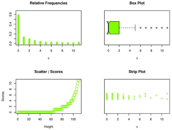
Figure 5.
Nonparametric data plots.
MLEs, standard errors (SEs), upper (U) and lower (L) confidence intervals (CIs) for the parameters, and goodness-of-fit measures (GOFMs) for kidney dysmorphogenetic data are reported in Table 3, Table 4 and Table 5.
Table 3.
GOFM for the dataset—Part I.
Table 4.
GOFM for the dataset—Part II.
Table 5.
GOFM for the dataset—Part III.
The DPa, DLogL, DIW, DLo and DB-II distributions worked quite well beside DWPLT. However, the DWPLT distribution was the best among all tested models. Figure 6 shows that the MLEs were unique because the estimator was monomorphic. We could not draw the contour diagram because the proposed model had only one parameter. Thus, the log-likelihood profile was sufficient to substantiate our claim.
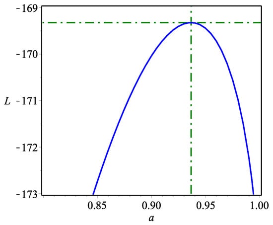
Figure 6.
L profile of the DWPLT parameter based on the dataset.
Figure 7 shows our empirical results reporting that DWPLT was more fit to analyze the data set I.
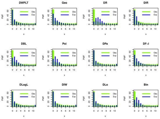
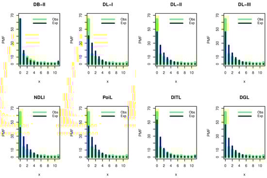
Figure 7.
Estimated PMFs for the dataset.
The moment estimator showed that the maximal-likelihood and moment estimators were equal and unique.
6. Results and Future Work
In this article, a new one-parameter discrete model was proposed, DWPLT, which is considered a generalization to the Poisson distribution. Some basic distributional characteristics of the presented distribution were derived in closed forms and are discussed. The DWPLT model was capable of modeling positively skewed leptokurtic data and describing hyperscattered data. Moreover, the hazard rate function decreased on the basis of the model parameter. Two estimation methods were applied to obtain the best estimator for the DWPLT parameter. Both approaches worked very well for this purpose across simulation schemes. The practical significance of the DWPLT distribution was demonstrated using a real medical dataset, and it was compared to other competitive lifetime distributions. The DWPLT model had more flexibility in fitting the dataset than that of the mentioned models. Lastly, DWPLT distribution could be useful in many applications, such as environmental studies, reliability theory, and actuarial and medical sciences. As future work, the regression model and time series analysis will be discussed.
Author Contributions
Conceptualization, M.S.E. and M.E.-M.; methodology, M.E.-D., M.S.E. and M.E.-M.; software, M.E.-M.; validation, M.E.-D.; formal analysis, M.S.E.; investigation, M.E.-M.; resources, M.E.-D.; data curation, M.S.E., M.E.-D. and M.E.-M.; writing—original draft preparation, M.S.E. and M.E.-M.; writing—review and editing, M.S.E.; visualization, M.S.E. and M.E.-M. All authors have read and agreed to the published version of the manuscript.
Funding
This research was funded by Research & Innovation of the Ministry of Education in Saudi Arabia grant number [IF-PSAU-2022/01/22580].
Data Availability Statement
All datasets are listed within the paper.
Acknowledgments
The authors extend their appreciation to the Deputyship for Research and Innovation of the Ministry of Education in Saudi Arabia for funding this research work through project number IF-PSAU-2022/01/22580.
Conflicts of Interest
The authors declare no conflict of interest.
References
- Yari, G.; Tondpour, Z. Some new discretization methods with application in reliability. Appl. Appl. Math. Int. J. (AAM) 2018, 13, 6. [Google Scholar]
- Roy, D. Discrete Rayleigh distribution. IEEE Trans. Reliab. 2004, 53, 255–260. [Google Scholar] [CrossRef]
- Krishna, H.; Pundir, P.S. Discrete Burr and discrete Pareto distributions. Stat. Methodol. 2009, 6, 177–188. [Google Scholar] [CrossRef]
- Gomez-Déniz, E. Another generalization of the geometric distribution. Test 2010, 19, 399–415. [Google Scholar] [CrossRef]
- Jazi, M.A.; Lai, C.D.; Alamatsaz, M.H. A discrete inverse Weibull distribution and estimation of its parameters. Stat. Methodol. 2010, 7, 121–132. [Google Scholar] [CrossRef]
- Al-Huniti, A.A.; AL-Dayian, G.R. Discrete Burr type III distribution. Am. J. Math. Stat. 2012, 2, 145–152. [Google Scholar] [CrossRef]
- Nekoukhou, V.; Alamatsaz, M.H.; Bidram, H. Discrete generalized exponential distribution of a second type. Statistics 2013, 47, 876–887. [Google Scholar] [CrossRef]
- Hussain, T.; Ahmad, M. Discrete inverse Rayleigh distribution. Pak. J. Stat. 2014, 30. [Google Scholar]
- Hussain, T.; Aslam, M.; Ahmad, M. A two parameter discrete Lindley distribution. Rev. Colomb. Estad. 2016, 39, 45–61. [Google Scholar] [CrossRef]
- Abebe, B.; Shanker, R.A. Discrete Lindley distribution with applications in biological sciences. Biom. Biostat. Int. J. 2018, 7, 48–52. [Google Scholar] [CrossRef]
- Al-Babtain, A.A.; Ahmed, A.H.N.; Afify, A.Z. A new discrete analog of the continuous Lindley distribution, with reliability applications. Entropy 2020, 22, 603. [Google Scholar] [CrossRef]
- Eliwa, M.S.; Altun, E.; El-Dawoody, M.; El-Morshedy, M. A new three-parameter discrete distribution with associated INAR (1) process and applications. IEEE Access 2020, 8, 91150–91162. [Google Scholar] [CrossRef]
- Almazah, M.M.A.; Erbayram, T.; Akdoğan, Y.; Al Sobhi, M.M.; Afify, A.Z. A new extended geometric distribution: Properties, regression model, and actuarial applications. Mathematics 2021, 9, 1336. [Google Scholar] [CrossRef]
- Poisson, S.D. Mémoire sur l’équilibre et le mouvement des corps élastiques. Mém. Acad. R. Sci. Inst. Fr. 1829, 8, 357–570. [Google Scholar]
- Del Castillo, J.; Pérez-Casany, M. Weighted Poisson distributions for overdispersion and underdispersion situations. Ann. Inst. Stat. Math. 1998, 50, 567–585. [Google Scholar] [CrossRef]
- Fisher, R.A. The effect of methods of ascertainment upon the estimation of frequencies. Ann. Eugen. 1934, 6, 13–25. [Google Scholar] [CrossRef]
- Dietz, E.; Bhning, D. On estimation of the Poisson parameter in zero-modified Poisson models. Comput. Stat. Data Anal. 2000, 34, 441–459. [Google Scholar] [CrossRef]
- Kokonendji, C.C.; Mizere, D.; Balakrishnan, N. Connections of the Poisson weight function to overdispersion and underdispersion. J. Stat. Plan. Inference 2008, 138, 1287–1296. [Google Scholar] [CrossRef]
- El-Morshedy, M.; Eliwa, M.S.; Altun, E. Discrete Burr-Hatke distribution with properties, estimation methods and regression model. IEEE Access 2020, 8, 74359–74370. [Google Scholar] [CrossRef]
- Wolfram Research. HurwitzLerchPhi Function. J. Appl. Stat. 2008, 32, 1461–1478. [Google Scholar]
- Altun, E.; El-Morshedy, M.; Eliwa, M.S. A study on discrete Bilal distribution with properties and applications on integervalued autoregressive process. Revstat-Stat. J. 2022, 20, 501–528. [Google Scholar]
- Poisson, S.D. Probabilité des jugements en matière criminelle et en matière civile, précédées des règles générales du calcul des probabilitiés; Bachelier: Paris, France, 1837; Volume 1, p. 1837. [Google Scholar]
- Eliwa, M.S.; El-Morshedy, M. A one-parameter discrete distribution for over-dispersed data: Statistical and reliability properties with applications. J. Appl. Stat. 2022, 49, 2467–2487. [Google Scholar] [CrossRef] [PubMed]
- Para, B.A.; Jan, T.R. Discrete version of log-logistic distribution and its applications in genetics. Int. J. Mod. Math. Sci. 2016, 14, 407–422. [Google Scholar]
- Para, B.A.; Jan, T.R. On discrete three parameter Burr type XII and discrete Lomax distributions and their applications to model count data from medical science. Biom. Biostat. J. 2016, 4, 1–15. [Google Scholar]
- Shanker, R.; Mishra, A. A two-parameter Poisson-Lindley distribution. Int. J. Stat. Syst. 2014, 9, 79–85. [Google Scholar]
- Almazah, M.M.A.; Alnssyan, B.; Ahmed, A.H.N.; Afify, A.Z. Reliability properties of the NDL family of discrete distributions with its inference. Mathematics 2021, 9, 1139. [Google Scholar] [CrossRef]
- Eldeeb, A.S.; Ahsan-Ul-Haq, M.; Babar, A. A discrete analog of inverted Topp-Leone distribution: Properties, estimation and applications. Int. J. Anal. Appl. 2021, 19, 695–708. [Google Scholar]
- El-Morshedy, M.; Altun, E.; Eliwa, M.S. A new statistical approach to model the counts of novel coronavirus cases. Math. Sci. 2022, 16, 37–50. [Google Scholar] [CrossRef]
- Chan, S.K.; Riley, P.R.; Price, K.L.; McElduff, F.; Winyard, P.J.; Welham, S.J.; Long, D.A. Corticosteroid-induced kidney dysmorphogenesis is associated with deregulated expression of known cystogenic molecules, as well as Indian hedgehog. Am. J.-Physiol.-Ren. Physiol. 2010, 298, F346–F356. [Google Scholar] [CrossRef] [PubMed]


Disclaimer/Publisher’s Note: The statements, opinions and data contained in all publications are solely those of the individual author(s) and contributor(s) and not of MDPI and/or the editor(s). MDPI and/or the editor(s) disclaim responsibility for any injury to people or property resulting from any ideas, methods, instructions or products referred to in the content. |
© 2023 by the authors. Licensee MDPI, Basel, Switzerland. This article is an open access article distributed under the terms and conditions of the Creative Commons Attribution (CC BY) license (https://creativecommons.org/licenses/by/4.0/).