Article

Research on the Mesoscopic Characteristics of Kelvin–Helmholtz Instability in Polymer Fluids with Dissipative Particle Dynamics

1
School of Mathematics and Statistics, Chongqing Three Gorges University, Chongqing 404020, China
2
School of Computer Science, Guangdong University of Science & Technology, Dongguan 523083, China
3
State Key Laboratory of Plateau Ecology and Agriculture, Qinghai University, Xining 810016, China
4
School of Sciences, Nanchang Institute of Technology, Nanchang 330099, China
5
Department of Computer Technology and Applications, Qinghai University, Xining 810016, China
*
Author to whom correspondence should be addressed.
Processes 2023, 11(6), 1755; https://doi.org/10.3390/pr11061755
Submission received: 9 May 2023 / Revised: 3 June 2023 / Accepted: 6 June 2023 / Published: 8 June 2023
(This article belongs to the Special Issue 10th Anniversary of Processes: Women's Special Issue Series)

Abstract

:
In this paper, the two-dimensional Kelvin–Helmholtz (KH) instability occurring in the shear flow of polymer fluids is modeled by the dissipative particle dynamics (DPD) method at the coarse-grained molecular level. A revised FENE model is proposed to properly describe the polymer chains. In this revised model, the elastic repulsion and tension are both considered between the adjacent beads, the bond length of which is set as one segment’s equilibrium length. The entanglements between polymer chains are described with a bead repulsive potential. The characteristics of such a KH instability in polymer fluid shear flow can be successfully captured in the simulations by the use of the modified FENE model. The numerical results show that the waves and vortexes grow more slowly in the shear flow of the polymer fluids than in the Newtonian fluid case, these vortexes become flat, and the polymer impedes the mixing of fluids and inhibits the generation of turbulence. The effects of the polymer concentration, chain length, and extensibility are also investigated regarding the evolution of KH instability. It is shown that the mixing of two polymer fluids reduces, and the KH instability becomes more suppressed as the polymer concentration increases. The vortexes become much longer with the evolution of the elongated interface as the chain length turns longer. As the extensibility increases, the vortexes become more flattened. Moreover, the roll-up process is significantly suppressed if the polymer has sufficiently high extensibility. These observations show that the polymer and its properties significantly influence the formation and evolution of the coherent structures such as the waves and vortexes in the KH instability progress.

1. Introduction

It is well known that Kelvin–Helmholtz (KH) instability occurs at the interface between two parallel streams with a relative velocity difference [1]. KH instability has been an interesting and challenging subject in that the interface undergoes a complex evolution. It should be noted that the KH instability can be encountered in the flow of both Newtonian [2] and non-Newtonian fluids [3,4,5]. This phenomenon is of fundamental importance in science research and engineering applications, such as marine science [6], turbulent mixing [7,8], air-assisted atomization [9], material friction [10], nuclear engineering [11], and so on.
So far, the majority of the KH instability studies are limited to Newtonian fluids [12,13,14,15,16,17,18,19,20,21]. That occurring in the flow of non-Newtonian fluids has rarely been researched. Cadot and Kumar [22] experimentally studied the viscoelastic effect on shear instabilities. Their results showed that the viscoelastic solutions drastically modified the instabilities. Azaiez and Hornsy [23] numerically investigated the effect of viscoelasticity on the free shear flow of viscoelastic liquids. They also simulated the roll-up of non-Newtonian free shear flow at high Reynolds numbers [24]. Kumar and Homsy’s simulations of the KH instability [25] showed how the addition of a polymer affected the transition to turbulence in free shear layers. In Yu and Phan-Thien’s simulations [26], the functions of the added polymer were discussed in detail. Richter et al. [27] simulated the three-dimensional viscoelastic flow pasting a circular cylinder and investigated the roll-up instability formed in the wake. Tiwari et al. [28] simulated the evolution of a shear flow structure in viscoelastic fluids with a generalized hydrodynamic model. They observed that the growth rate of the KH instability diminished with the increasing phase velocity of the transverse wave. In these numerical simulations, the fluid flows are just roughly described with a macroscopic continuum model.
As a great deal of interest is focused on the physical phenomena and industrial applications that involve the complex flow at a small scale, it is of great importance to understand the KH instability occurring in the non-Newtonian fluids at a mesoscale. As the system scale decreases, thermal fluctuations have a greater influence on the fluid dynamics. What is worse, continuum formulations based on partial differential equations, i.e., the Navier–Stokes equations, are even unable to describe the KH instability problem at such scale without modifications. As a mesoscopic simulation method, the lattice Boltzmann method (LBM) may be employed to model the vortex formation at a small scale for the KH instability problem [29,30,31,32]. However, it does not work when modeling the transition from laminar flow to turbulence due to the restriction of the lattice. These characteristics of complex fluids at a small scale may also be modeled by the use of molecular dynamics (MD) [33,34]. However, MD simulation needs too high of a calculation load to model routine problems [35]. Hence, dissipative particle dynamics (DPD) are considered to be the first choice for investigating the KH instability that occurs in the flow of polymer fluids in this work.
DPD is a coarse-grained method that connects microscopic and macroscopic worlds. This method was originally conceived as a mesoscale technique for simulating fluid systems by Hoogerbrugge and Koelman [36]. Subsequently, Español and Warren [37] and Marsh [38] established a wholesome theoretical basis for DPD based on statistical mechanics. In recent years, as the small-scale technologies developed fast, DPD has attracted increasing attention, and its applications have been rapidly extended to various research fields. These applications include colloidal suspension [39], liquid–liquid two-phase flow [40], gas–liquid two-phase flow [41], electroosmotic flow [42], liquid nanojets [43], solid–liquid interactions [44], particle sedimentation [45], blood flow [46], colloid transport in porous media [47], oil-in-water emulsion [48], magnetorheological fluids [49], etc. In contrast to these aspects, the applications of DPD in polymer systems are more extensive, such as polymer solutions [50], macromolecular suspension [51,52], topological entanglements in polymer melts [53,54], the phase behavior of polymer melts [55], the scaling behavior of polymers [56], and so on. For more details about the DPD method, see Moeendarbary et al. [57] and Liu et al. [58]. It should be noted that the DPD method has also been applied to study the phenomenon of fluid instability at the mesoscopic particle level [59,60,61,62,63,64], but most of them just considered the instability occurring in the flow of simple fluids.
Polymer fluids are non-Newtonian fluids with polymers. Polymers usually have long polymer chains and a large molecular weight. According to the concentration of polymers, polymer fluids can be divided into polymer melts, polymer concentrated solutions, and polymer dilute solutions. Polymer chains in polymer fluids can produce interactions such as entanglement and interpenetration, which affect the rheological properties of polymer fluids. For the high-concentration polymer fluids, the interaction forces between molecules are strengthened. The entanglement and interpenetration between polymer chains are also enhanced, making the rheological properties of polymer fluids more complex.
Studying the KH instability that occurs in the flow of non-Newtonian fluids such as polymer fluids will gain good cognition of non-Newtonian fluids’ effect on the instability in complicated flows, especially at a small scale. For investigating the dynamic behaviors of polymer fluids, such as KH instability, it is important to construct an effective model for describing the polymers. In simulations of polymers at micro- or meso-scales, the extendable non-linear elastic (FENE) chain is widely used owning to its vivid description of the polymer chain motion. The drawback of the traditional FENE chain model is that it only considers the elastic tension between adjacent beads of a chain; the elastic repulsion, however, is ignored [65,66].
This article presents a modified FENE chain model in which the interaction between adjacent beads is determined with consideration of both elastic tension and elastic repulsion. The entanglement model is given and employed in the simulations.

2. Problem Setup

The two-dimensional rectangle computational domain is  Ω = L / 2 , L / 2   ×   [ H / 2 , H / 2 ] , where the length of the computational domain  L  is chosen to be quadruple the domain height  H . The computational domain for the KH instability problem is represented by a set of particles with an equidistant particle distribution. At the beginning of the simulation, the computational domain is halved by a midline  y = 0 , where each half represents the different fluid regions with the same number of particles. Initially, the particles of two-layer fluids are set into thermal motion and superposed shear velocities in opposite directions with the same magnitude, that is:
U = u 0                         y 0 u 0                   y < 0
where  u 0  is the magnitude of shear velocities. Periodic boundary conditions are implemented at  x = L / 2  and  x = L / 2 , and wall boundary conditions are implemented at  y = H / 2  and  y = H / 2 , where each solid wall is represented by two rows of wall boundary particles, setting their velocities to  u 0  and  u 0 , correspondingly, throughout the simulation. The no-slip boundary conditions on boundary walls are implemented by Maxwellian reflection. In addition, it should be pointed out that in the DPD simulation, thermal fluctuations can spontaneously initiate the interface instability in shear flow, unlike the macroscopic continuum model in which initial sinusoidal perturbations are artificially implemented to the fluid–fluid interface.

3. DPD Method and Polymer Model

3.1. The DPD Method

In DPD simulation, the fluids are modeled by a system of particles, and the motions of these DPD particles are governed by Newton’s second law of motion. The motion of particle  i  is determined as [67]
d r i d t = v i
m i d v i d t = F i
where  r i  is the particle position,  v i  is the particle velocity,  m i  is the particle mass, and  F i  is the resultant force exerted on the particle  i  by all the other particles. In the standard DPD model, the resultant force  F i  contains three parts: the conservative force  F i C , the dissipative force  F i D  and the random force  F i R , which are pairwise and center-to-center. The resultant force  F i  is written as [67]
F i = j i F i j C + j i F i j D + j i F i j R
where the conservative force  F i j C  is a soft repulsive force acting along the line of centers.  F i j C  is calculated as [67]
F i j C = a i j w C r i j   e i j
w C r i j = 1 r i j r c           r i j r c 0                             r i j > r c
where  a i j  is a parameter representing the strength of a repulsive force,  r i j = r i r j  is the relative position vector between particle  i  and particle  j r i j = r i j e i j  is a unit vector given by  e i j = r i j / r i j r c  is the cutoff radius, and  w C r i j  is the weight function for conservative force.
In order to simulate liquid–liquid interface with the DPD method, Groot and Warren [67] have made a link between the repulsion parameter and Flory–Huggins theory. For the number densities  n = 3  and  n = 5 , they have also obtained the relationships between the Flory–Huggins parameter  χ  and the repulsion parameter  a i j  for two-type particles. Subsequently, AlSunaidi et al. [68] have obtained the relationship between  χ  and  a i j  for the number density  n = 4  by interpolating the equations provided for number densities  n = 3  and  n = 5 , that is [62]:
a i j = α                                         if   particles   i   and   j   are   the   same   type   particle α + 2.05 χ             if   particles   i   and   j   are   different   type   particles
So, as far as two-dimensional simulation is considered, initially, two particles are used for each square cell, which corresponds to the face-centered cubic with four particles per cubic lattice in a three-dimensional system. The size of the square cells and cubic lattices keeps unit, which means the side length of all the cells and lattices is equal to 1, and the corresponding number density is 4. Therefore, in our simulation, the number density can be deemed as  n = 4 , and Equation (7) is taken to model the binary fluids. When the Flory–Huggins parameter  χ  is positive, the binary fluids are immiscible, while they are miscible when it is zero or negative.
In Equation (4),  F i j D  is calculated as [67]
F i j D = γ w D r i j e i j v i j   e i j
where,  γ  is the strength of the dissipative force,  w D r i j  is the weight function for  F i j D , and  v i j = v i v j  is the relative velocity.  F i j R  is calculated as [67]
F i j R = σ   w R r i j   ζ i j e i j
where  σ  is the strength of random force,  w R r i j  is the weight function for  F i j R v i j = v i v j  is the relative velocity, and  ζ i j  is the stochastic variable with the properties [67]
ζ i j = 0
ζ i j t   ζ i j t = δ i i δ j j + δ i j δ j i   δ t t
where     denotes an ensemble average and  δ i j  is the Kronecker delta.
This is according to the fluctuation dissipation theorem [67]
w D r i j = w R 2 r i j
and
σ 2 = 2 γ k B T
where  k B T  is the Boltzmann temperature of the system. The conventional dissipative weight function is adopted as [67]
w D r i j = w R 2 r i j = 1 r i j r c 2                       r i j r c 0                                                     r i j > r c
As can be seen from (12) and (14), the cutoff radii for the dissipative force should be equal to that for the random.

3.2. The Polymer Model

The adjacent particles on a polymer backbone can be linked together by the FENE spring force as follows [66].
F i j S = H S   r i j 1 r i j / r max 2  
where  H S  is the spring coefficient,  r i j = r i r j r i j = r i j r i , and  r j  denote the position vectors of bead  i  and bead  j , and  r max  refers to the maximum extensibility of one chain segment. However, the spring force (15) describes only the elastic tension, and the elastic repulsion is neglected.
To model the polymer chain more veritably, a modified FENE spring force [69] is adopted as follows.
F ¯ i j S = H S r i j r b o n d   r i j 1 r i j / r max 2 r max r b o n d
where  r b o n d  represents the bond length, and other physical quantities have the same meaning as the corresponding parameters in the original model (15). Figure 1 shows the schematic diagram of the elastic tension and repulsion in a polymer chain.
In polymer fluids, the uncrossability constraint creates entanglements when the chains try to cross each other, as shown in Figure 2. At present, there are some effective models that have been developed to deal with the bond crossing problem. Goujon et al. [70] and Sirk et al. [71] used a segmental repulsive potential to model polymer entanglements in DPD simulation. In order to avoid bond crossing in a two-dimensional system, Liu et al. [72] added a rigid core to each chain bead to prevent the beads from penetrating each other.
In this work, the above method is also employed, and a repulsive force with the same functional form as the DPD conservative potential is given as follows [63]:
F i j E = a i j E 1 r i j r c E   e i j             r i j r c E 0                                                             r i j > r c E
where  F i j E  is a force acting between beads  i  and  j  which belong to different chains with the distance  r i j , and it is called the entanglement force,  a i j E  is the controlling parameter for the entanglement force,  r c E  represents the cutoff value for the entanglement interactions, and the entanglement cutoff distance should be less than the cutoff distance for traditional DPD forces.

3.3. Integration Algorithms

Newton’s equations of motion (Equations (2) and (3)) are discretized with a modified version of the velocity–Verlet algorithm, including Equations (18)–(21):
r i t + Δ t = r i t + v i t Δ t + 1 2 Δ t 2 v ˙ i t
v ˜ i t + Δ t = v i t + λ Δ t v ˙ i t
v ˙ i t + Δ t = v ˙ i r i t + Δ t ,   v ˜ i t + Δ t
v i t + Δ t = v i t + 1 2 Δ t v ˙ i t + v ˙ i t + Δ t
where  Δ t  is the DPD time step, and  v ˙ i  is the particle acceleration caused by the forces adding to particle  i  from all other particles. The intermediate velocity  v ˜ i t + Δ t  is predicted before the forces are updated, and then this value is corrected at the end of each integration step;  λ  is an empirical parameter, and  λ = 0.65  is taken as the optimum value [67]. Here, the modified velocity–Verlet algorithm ((18)–(21)) is based on the Euler method to discretize Newton’s second law equations, so it is stable. To analyze the convergence rate of the modified velocity–Verlet algorithms (18)–(21), Taylor expansions were performed on displacement and velocity, respectively
r t + Δ t = r t + v t Δ t + Δ t 2 2 v ˙ t + O Δ t 3
v t + Δ t = v t + v ˙ t Δ t + O Δ t 2
It can be seen from (22) and (23) that the displacement is third-order convergence, and the velocity is at least first-order convergence. In addition, the mass of each particle is fixed, and the number of particles is constant in the simulation. Thus, the calculation system is mass conservation. The momentum of the system is related to the dissipated force, which consumes some momentum, and the boundary velocity, which supplements some momentum. Although the system does not maintain absolute conservation of momentum, the momentum fluctuations are so small that it can be considered basically conserved. In addition, for all calculations conducted in this study, the control equations and the results are represented by dimensionless variables using the reference mass, length, and energy, i.e., the particle mass  m , the side length  l  of the unit mesh, and the Boltzmann temperature  k B T .

4. Simulation Results and Discussion

4.1. KH Instability in Newtonian Fluids

Consider the KH instability occurring in the flow of Newtonian fluids with twofold purposes. One is to verify the DPD code for the KH instability problem, and the other is to provide a counterpart as a contrast for the case of polymer fluids that is mainly discussed in this work. The KH instability in two-component Newtonian fluids is simulated with the initial stream velocity:
U = 1                         y 0 1                   y < 0
It is on the domain Ω = [–500, 500] × [−126, 126]. In this two-dimensional system, the triangular lattice with two particles per unit cell is adopted in the initial coordinates. The right and left boundaries are the periodic boundary; the top and bottom boundaries are the wall boundary, and each wall boundary is composed of two layers of particles. The fluid particle number is 500,000, and the wall particle number is 4000. In this simulation, the two-component fluids have the same density, and the remaining parameter values are  α = 18.75 γ = 4.5 r c = 1.125 k B T = 1 χ = 5 , and  Δ t = 0.01 . As discussed in the literature [73], the gravitation is neglected in this test.
Figure 3 gives the temporal evolution of the fluid particles to illustrate the evolution of the KH instability occurring in the flow of Newtonian fluids. The upper layer of the fluids moves in the positive direction, while the lower layer of the fluids moves in the negative direction. There exists distinct penetration between both fluids. Early meso-level inter-diffusion causes a broadening of the interface, where meso-level thermal fluctuations perturb the interface and trigger the growth of small waves. As time goes on, these small waves grow in amplitude. Then, both fluids tend to gain horizontal velocity opposite to their initial bulk velocities and eventually crest to form small vortices. As the KH instability grows in the y-axis direction, the wavelength of the waves and vortices grows in the x-axis direction. Initially, small vortices grow with short wavelength modes, but ultimately, the larger vortex structures grow at the expense of the small ones. This process results in the formation of vortices, and the characteristic form of KH instability becomes much more pronounced at a later time. The roll-up interface dynamics are qualitatively consistent with those in the previous experiments [12] and simulations [33].

4.2. KH Instability in Polymer Fluids

The KH instability occurring in the flow of polymer fluids is a more complex physical process than that in the Newtonian fluids, which will be discussed in the following content. As mentioned earlier, Equations (16) and (17) are used for the polymer solution. Here, the spring coefficient  H S = 4.5 , the bond length  r b o n d = 2 / 2 , the maximum extensibility of one chain segment  r max = 2.5 r b o n d , the chain length  Χ n = 4 , the polymer concentration  c = 40 % , the entanglement force controlling parameter  a i j E = 8 , the entanglement cutoff distance  r c E = 0.8 r c , and other parameter values are similar to those used in the Newtonian case.
Figure 4 shows the instantaneous snapshots of the fluid particles to illustrate the evolution of the KH instability occurring in the flow of polymer fluids. In the initial time  t = 0 , the shear flow starts with the upper-layer fluid moving in a positive horizontal direction with bulk velocity  U = 1  and the lower-layer fluid moving in the opposite direction with bulk velocity  U = 1 . Subsequently, the interface disturbance generates spontaneously due to the thermal fluctuations, and the flow system becomes unstable. Similar to the Newtonian case, because of the shear action and the thermal disturbance, the lower-layer fluid starts moving in a positive vertical direction, whereas the upper-layer fluid starts moving in the opposite direction. As a result, both polymer fluids begin to penetrate each other. During this initial period, unlike the Newtonian case that generates many small vortexes near the original interface, it is difficult to form small vortexes in the shear flow of polymer fluids on account of the inhibition of the polymer. Instead, the interface instability occurring in the flow of polymer fluids manifests itself as some finger-like structures and needle-like structures developing at the interface. As time progresses, these finger-like structures and needle-like structures break and merge. Gradually, some waves generate at the interface with a long wavelength, which subsequently roll up and form vortexes. In contrast with the Newtonian case, the two polymer fluids have a lower mixing level, and the curly interface is significantly elongated and does not break up. This is because the polymer chains make the liquid micelles connect together. In the Newtonian case, under shear flow, the interface becomes more incompact and manifests plume-like structures, namely, the stream gradually changes from laminar flow to turbulence. However, the vortex structures in the polymer fluids are compact cluster structures instead of plume-like patterns. Thus, it can be seen that the polymer suppresses the growth of turbulence. Due to the inhibiting effect of the polymer on the interface instability, it needs more time to generate the waves and vortexes, and these vortex structures are flattened compared to the Newtonian ones. Our simulation results are consistent with previous experimental and numerical research revealing that the polymer inhibits the roll-up process [22,25,27].
Figure 5 shows the flow velocity in the vertical direction of Newtonian fluids and polymer fluids. In particular, the suppression influence of the polymer on the formation of small vortexes is clearly reflected in vertical velocity (see the top frames of Figure 5). In the initial, for the Newtonian case, many small vortexes appear near the original interface, where a small red zone (left, up-flow velocity) and a small blue zone (right, down-flow velocity) correspond to a vortex (see the top frame of Figure 5a). However, the vertical velocity is very small in the polymer case since there is almost no small vortex appearing at the interface (see the top frame of Figure 5b). In the late, the interface forms some large vortex structures, and the high vertical velocity is generated in the polymer fluids, which is just slightly lower than the Newtonian case (see the bottom frames of Figure 5). In conclusion, due to the inhibition of the polymer, the vortex of Newtonian fluid is formed earlier, while the vortex of polymer fluid is formed later. The vortex velocity of polymer fluid is smaller than that of Newtonian fluid at the same time point. Here, in order to reduce the random noise, the values are averaged over multiple steps to obtain the results at the midpoint of the time interval for the vertical velocity, and so are the horizontal velocity and velocity vector-field in subsequent sections.
Figure 6 presents the vortex growth occurring in Newtonian fluid and polymer fluid, which are mean values that are obtained by averaging the vortex growth for several instances. From this figure, it can be seen that the vortexes develop more quickly in Newtonian fluid than they do in polymer fluid.
The above phenomenon can be explained by the following. When the molecular chain of a polymer is in a flow field with a velocity gradient caused by shear rate changes, each part of the long chain may be in different velocity regions: one end may be in the faster velocity region, while the other end may be in the slower velocity region, and even the flow velocity direction may be opposite in different regions where different parts of the molecular chain are located. At this point, relative movement occurs at both ends of the molecular chain, which may cause stretching and orientation of the molecular chain. The molecular chain interacts with the fluid during stretching and orientation, resulting in the HK vortex being stretched and flattened.

4.3. Effect of Polymer Concentration

To investigate the effect of polymer concentration, the same initial velocity conditions and other parameter values were used to create Figure 4, except for the concentration. Consider the fluid particles, velocity vector-field, horizontal velocity, and vertical velocity for the concentrations of  c = 10 % c = 30 % , and  c = 70 % , respectively. In our simulations, the vortexes that reach saturation can be captured before  t = 700 . However, it is much later for  c = 70 %  to form a vortex.
Figure 7 shows the fluid particles, velocity vector-field, horizontal velocity, and vertical velocity. In the case of  c = 10 % , as the upper shear layer moves in a positive level direction and the lower shear layer moves in the opposite direction, the waves generate, grow, coalesce, get larger, and form vortexes, as expected. In this case, the wave evolution and the vortex roll-up process are similar to what are seen in the Newtonian case, but the vortexes are slightly flattened relative to the Newtonian ones. As the polymer concentration increases,  c = 30 % , the polymer stabilizing effect on the interface evolution becomes obvious. The formation of the wave and vortex patterns is slightly postponed in contrast to the foregoing case, and the vortexes become more flattened. For a higher polymer concentration,  c = 70 % , at the beginning, the waves develop in the vertical direction with a small increasing amplitude. As time progresses, the vertical growth of the waves becomes slower and slower. Instead, finger-like structures begin to develop and are almost parallel to the horizontal direction. Gradually, these finger-like structures are elongated. At last, these finger-like structures break up and form some drops. The vortex patterns are not seen at any time. One can easily notice that, with the polymer concentration increasing, the mixing of two polymer fluids reduces, the KH instability becomes more suppressed, and the vortex formation is delayed to a later simulation time. Peculiarly, for the case of a high polymer concentration, the vortex structures are completely inhibited at the mesoscopic level. The effect of the polymer concentration on the KH instability is also reflected in the fluid velocity. As the polymer concentration increases, eddy velocities weaken. In particular, when the polymer concentration rises to  c = 70 % , the vertical velocity is very small, and almost no eddy current can be observed in the velocity vector-field. Here, the simulation results are consistent with the notion that the polymer can inhibit the formation of concentrated regions of the vortex [25].
This arises due to the complex interaction between the molecular chains. As the concentration of the polymer increases, the number of polymer molecules increases, and the interactions between molecular chains become frequent. It is the process of entanglement and unwinding in the molecular chains that hinders the formation and development of KH vortices.

4.4. Effect of Chain Length

Consider the effect of chain length on the evolution of KH instability. Here, the polymer concentration is 30%. The same initial velocity conditions and other parameter values were utilized to produce Figure 4, except for the chain length. Consider in the following the fluid particles, velocity vector-field, horizontal velocity, and vertical velocity at the moment that the vortexes reach saturation for the chain lengths of  Χ n = 2 Χ n = 8 , and  Χ n = 30 , respectively.
Figure 8 shows snapshots of the fluid particles, velocity vector-field, horizontal velocity, and vertical velocity at the moment that the vortexes reach saturation. In the case of  Χ n = 2 , i.e., the FENE dumbbell model, at the early time, some small waves form at the interface, which grow in the vertical direction with increasing amplitude. Gradually, these waves merge and evolve into vortexes with a larger amplitude. This process is very similar to the Newtonian case. In the case of longer chains,  Χ n = 8 , it can be observed that the waves grow and roll up with a slower rate relative to the case of  Χ n = 2 . The vortexes grow up with a small altitude, which are elongated by following the evolution of the shear flow. When the chain length becomes much longer,  Χ n = 30 , the interface roll-up is seriously retarded, the formation of vortexes needs more time, and the vortexes become longer with the evolution of the elongated interface. From the velocity vector-field, horizontal velocity, and vertical velocity, it can be seen that with the chain length increasing, the eddy currents weaken markedly.
The flow characteristics of polymer fluids are closely related to the structure of molecular chains. Long-chain molecular structures involve a wide range of flow regions, and long-chain molecules are more prone to entanglement. Therefore, large vortices are easily generated under the interaction of these long-chain molecules and fluid molecules. In addition, these long-chain molecules undergo stretching and orientation under shear, which simultaneously react on the fluid, causing the vortices to flatten.

4.5. Effect of Polymer Extensibility

When the polymer concentration is 30%, the same initial conditions and other parameter values are adopted to create Figure 4, except for the parameter  r max . Figure 9 shows snapshots of the fluid particles, velocity vector-field, horizontal velocity, and vertical velocity for the extensibilities of  r max = 2 r b o n d r max = 7 r b o n d , and  r max = 20 r b o n d , respectively. For  r max = 2 r b o n d  and  r max = 7 r b o n d , these snapshots are captured at the moment that the vortexes reach saturation. For  r max = 20 r b o n d , the snapshots are captured at a certain moment in a later stage. For the case of  r max = 2 r b o n d , the roll-up vortexes and the mixing of two fluids are similar to what are seen in the lower-concentration and Newtonian cases. However, for the higher extensibility,  r max = 7 r b o n d , it is obviously postponed to form the vortex structures, and the roll-up vortexes appear to be strongly flattened relative to the vortexes at  r max = 2 r b o n d . This flattening is somewhat similar to what is seen for an increasing chain length. The simulations are consistent with the results of Kumar and Homsy [25], which show that the roll-up process is significantly suppressed if the polymer has sufficiently long extensibility. When the parameter  r max  further increases,  r max = 20 r b o n d , the roll-up process of the interface is significantly inhibited. For this case, at the early time, the waves grow in the vertical direction with a small amplitude and, at the same time, merge in the horizontal direction. As time goes by, the vertical growth of the waves gradually slows down. Their horizontal growth goes on as the finger-like structures are elongated longer and longer. It is also observed that a high extensibility reduces eddy velocities.
For molecular chains with high extensibility, the stretching deformation scale of the molecular chain is larger under shear, and the deformation relaxation time is longer, which means that the molecular chains with orientation during flow do not easily restore their original shape. Therefore, under the interaction of these highly extensible molecular chains with fluids, vortices become flatter and even develop into finger-like structures.

5. Summary and Conclusions

The KH instability occurring in the shear flow of polymer fluids is numerically researched using DPD at the mesoscopic molecular level. The polymer chains are modeled with the modified FENE model that describes both the elastic tension and the elastic repulsion between the adjacent beads with the bond length as the equilibrium length of one segment. Meanwhile, the entanglements between polymer chains are modeled with a simplified bead repulsive potential. The following results are obtained through numerical simulation.
(1)
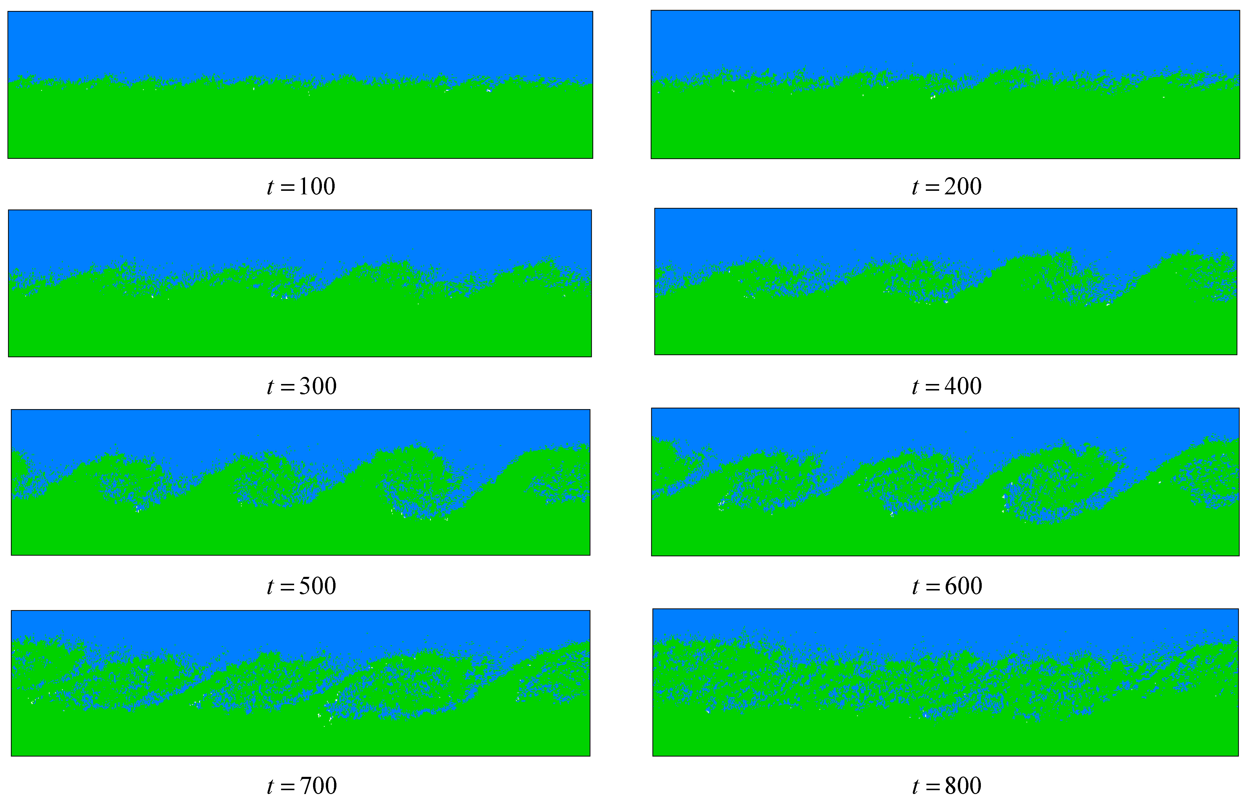
The DPD algorithm is validated by simulating the KH instability that occurs in the shear flow of Newtonian fluids, and the mesoscopic results of the present simulation for Newtonian fluids are qualitatively consistent with previous experimental and numerical results.
(2)
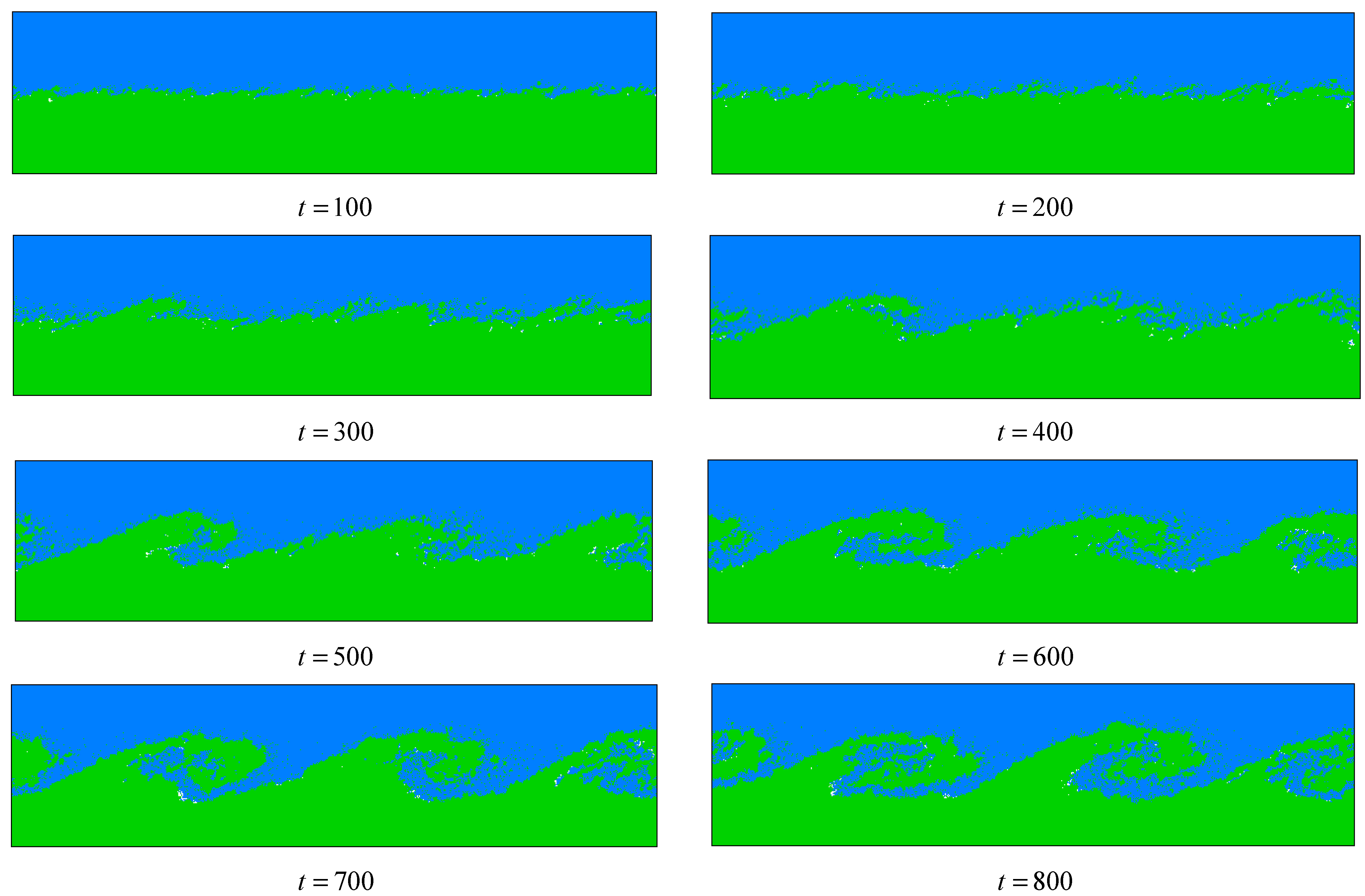
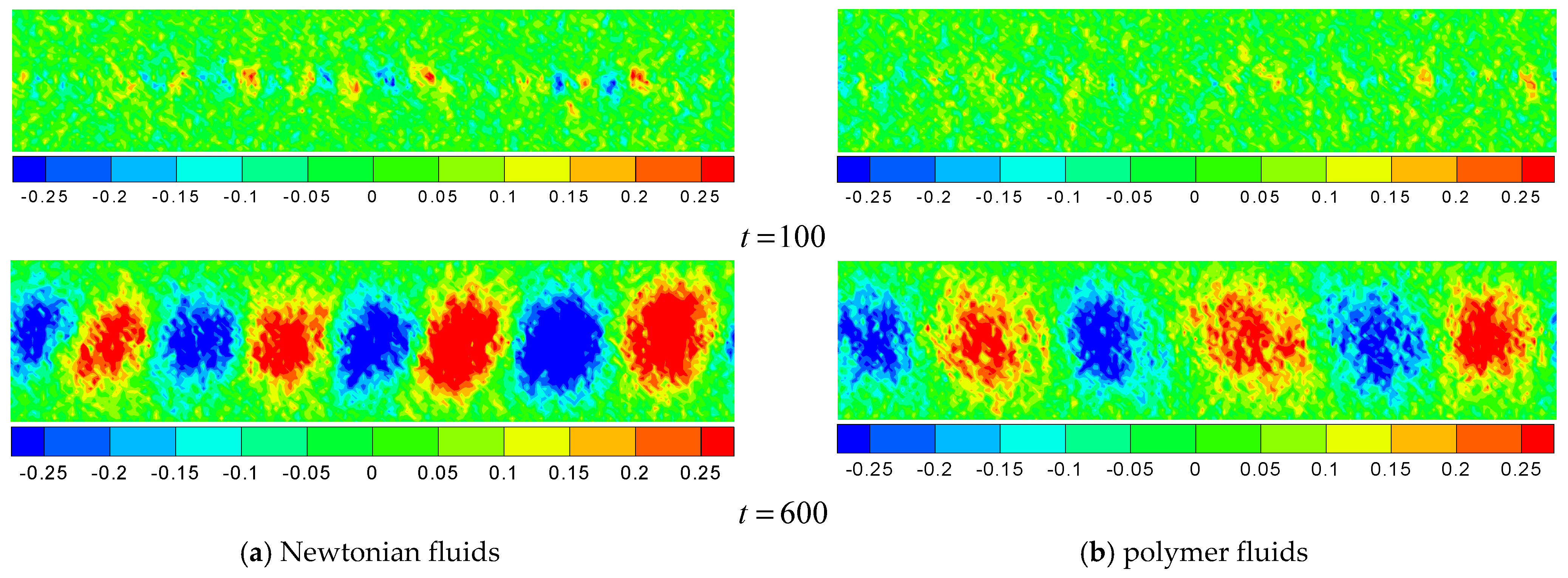
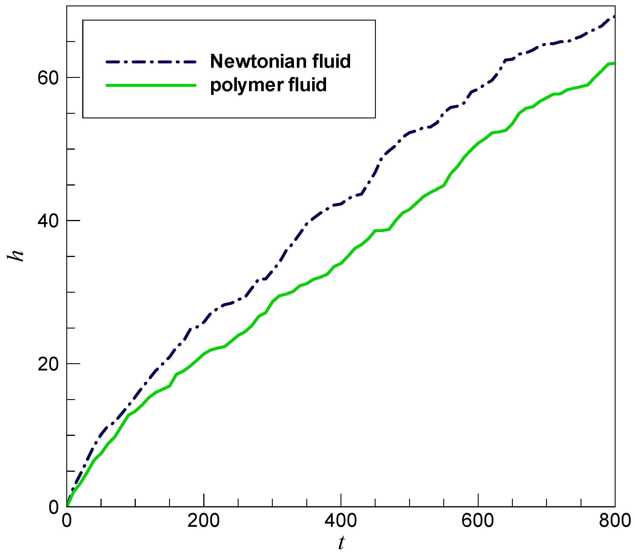
The characteristics of the KH instability that occurs in the flow of polymer fluids are explored with the validated DPD code. It is shown that, in contrast with their Newtonian counterparts, the waves and vortexes forming in the shear flow of polymer fluids grow more slowly, and these vortexes are flattened. In particular, the roll-up interface is conspicuously elongated and does not break up due to the reason that the polymer chains make the liquid micelles join together. Thus, the polymer hinders the mixing of fluids and suppresses the generation of turbulence. It is also observed that there is almost no small vortex appearing in the development process of the KH instability due to the inhibition of the polymer.
(3)
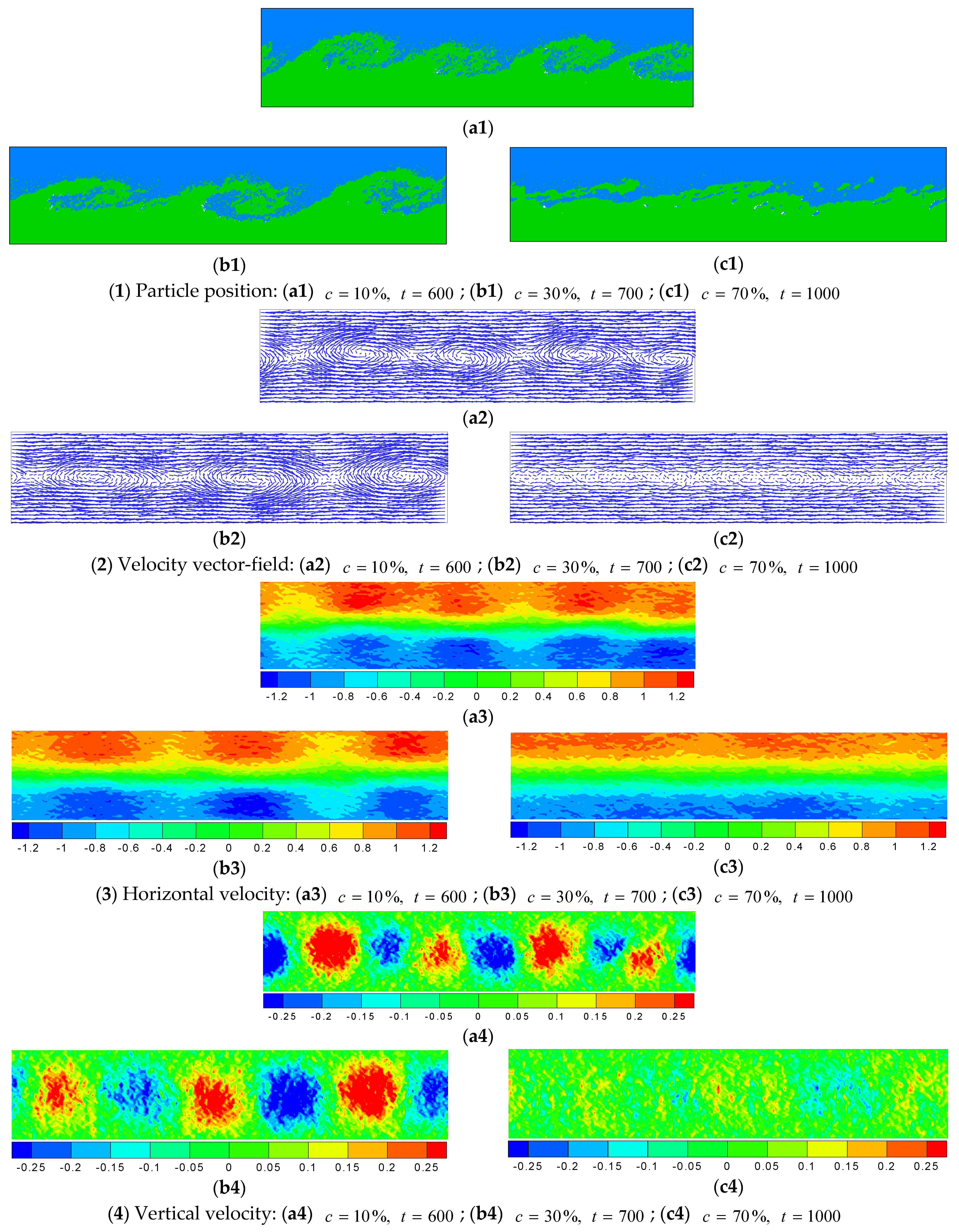
The effects of the polymer concentration on the KH instability are researched. The results show that with the polymer concentration increasing, the inhibitory effect becomes more conspicuous, the mixing of two polymer fluids reduces, and the transition from laminar to turbulence is even more restrained.
(4)
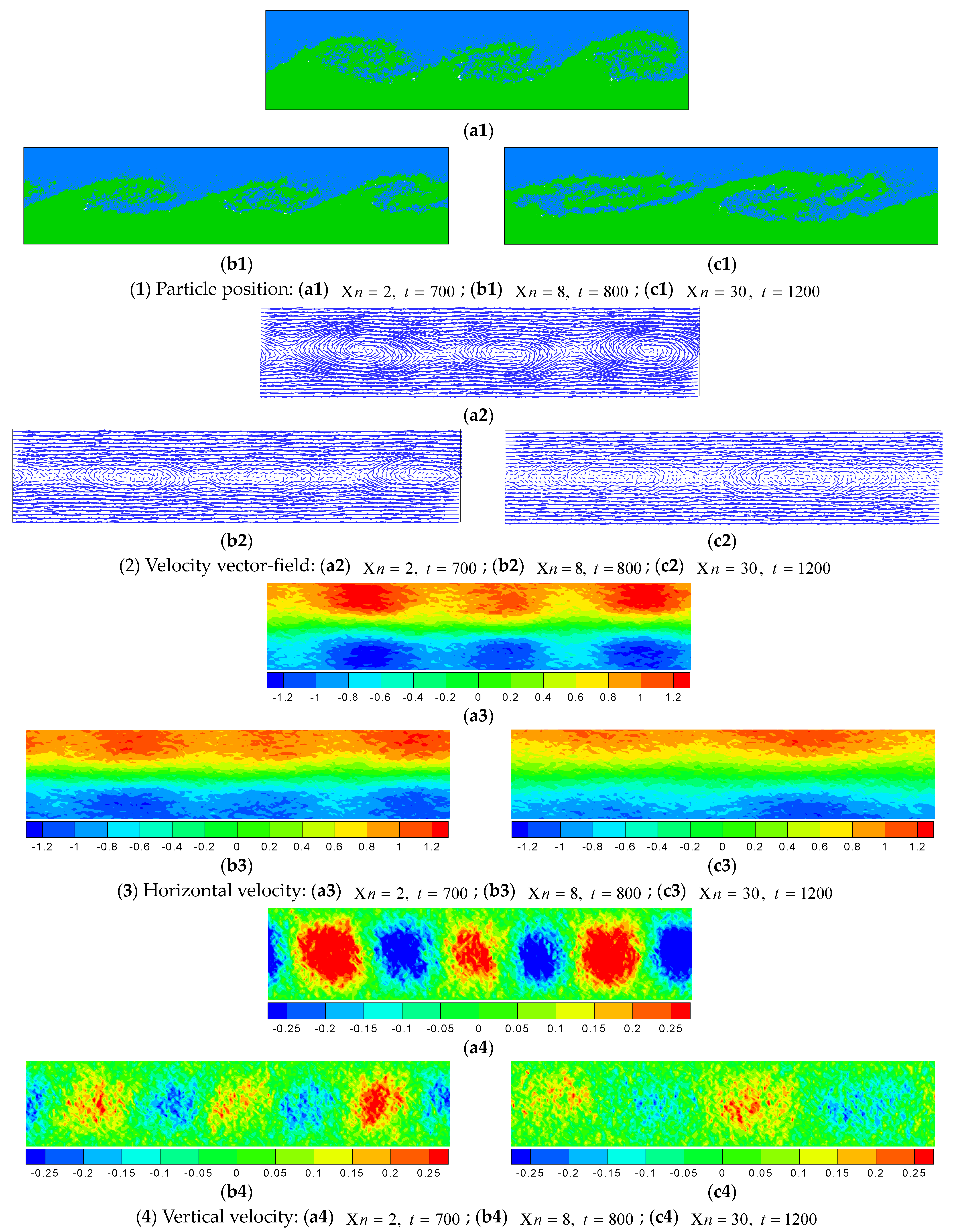
The effects of the chain length and extensibility of the polymer on the KH instability are also investigated. For the case of a long chain or high extensibility, the effect of the polymer on the flow structure is more profound. When the chain length gets longer, even the concentration remains constant, the formation of the waves and vortexes is delayed to a later simulation time, and the vortexes become longer and more flattened. This kind of situation also occurs when the polymer extensibility increases. The most striking effect of the high extensibility is the complete suppression of all vortex structures.

Author Contributions

Conceptualization, G.W. and Y.L; methodology, G.W. and Y.L; software, G.W.; validation, G.W. and H.W.; formal analysis, G.W.; investigation, G.W. and Y.L; resources, G.W.; data curation, G.W.; writing—original draft preparation, G.W.; writing—review and editing, G.W.; visualization, G.W.; supervision, S.L. and Y.L.; project administration, Y.L. All authors have read and agreed to the published version of the manuscript.

Funding

This research received funding from the National Natural Science Foundation of China (61962051), the Science and Technology Plan Project of Qinghai Province—Applied Basic Research Plan (2023-ZJ-736), the Open Project of State Key Laboratory of Plateau Ecology and Agriculture, Qinghai University (2021-ZZ-02), the Jiangxi Provincial Natural Science Foundation (No. 20212BAB201020), the National Natural Science Foundation of China (No. 12161058), and the Youth Foundation Program of Qinghai University (No. 2020-QGY-11).

Institutional Review Board Statement

Not applicable.

Informed Consent Statement

Not applicable.

Data Availability Statement

The data presented in this study are available on request from the corresponding author.

Conflicts of Interest

The authors declare no conflict of interest. The funders had no role in the design of the study; in the collection, analyses, or interpretation of the data; in the writing of the manuscript; or in the decision to publish the results.

Nomenclature

a i j coefficient of conservative force
a i j E coefficient of entanglement force
c concentration
F i resultant force
F i j C conservative force
F i j D dissipative force
F i j R random force
F ¯ i j S spring force
F i j E entanglement force
H height of computational domain
H S coefficient of spring force
k B T Boltzmann temperature
l side length of the unit cell
L length of the computational domain
m i particle mass
r i particle displacement
r b o n d bond length
r c cutoff radius
Δ t time step
t time
U boundary shear velocity
v i particle velocity
X n chain length
χ Flory–Huggins parameter
γ coefficient of dissipative force
λ empirical coefficient
σ coefficient of random force
Ω computational domain

References

  1. Fu, Y.; Qin, H. The physics of spontaneous parity-time symmetry breaking in the Kelvin–Helmholtz instability. New J. Phys. 2020, 22, 083040. [Google Scholar] [CrossRef]
  2. Gan, Y.; Xu, A.; Zhang, G.; Lin, C.; Lai, H.; Liu, Z. Nonequilibrium and morphological characterizations of Kelvin–Helmholtz instability in compressible flows. Front. Phys. 2019, 14, 43602. [Google Scholar] [CrossRef] [Green Version]
  3. Fu, Q.; Deng, X.; Yang, L. Kelvin–Helmholtz instability of confined Oldroyd-B liquid film with heat and mass transfer. J. Non-Newton. Fluid Mech. 2019, 267, 28–34. [Google Scholar] [CrossRef]
  4. Awasthi, M.K. Kelvin–Helmholtz instability of viscoelastic liquid-viscous gas interface with heat and mass transfer. Int. J. Therm. Sci. 2021, 161, 106710. [Google Scholar] [CrossRef]
  5. Farajzadeh, R.; Bayareh, M. Numerical study of Kelvin–Helmholtz instability of Newtonian and non-Newtonian fluids. AUT J. Mech. Eng. 2022, 6, 249–260. [Google Scholar]
  6. Kanarska, Y.; Shchepetkin, A.; McWilliams, J.C. Algorithm for non-hydrostatic dynamics in the Regional Oceanic Modeling System. Ocean Model. 2007, 18, 143–174. [Google Scholar] [CrossRef]
  7. Lesieur, M. Turbulence in Fluids; Kluwer Academic: Dordrecht, The Netherlands, 1997. [Google Scholar]
  8. IJzerman, W.L.; van Groesen, E. Low-dimensional model for vortex merging in the two-dimensional temporal mixing layer. Eur. J. Mech.-B/Fluids 2001, 20, 821–840. [Google Scholar] [CrossRef]
  9. Marmottant, P.; Villermaux, E. On Spray Formation. J. Fluid Mech. 2004, 498, 73–111. [Google Scholar] [CrossRef] [Green Version]
  10. Kim, H.J.; Karthikeyan, S.; Rigney, D. A simulation study of the mixing, atomic flow and velocity profiles of crystalline materials during sliding. Wear 2009, 267, 1130–1136. [Google Scholar] [CrossRef]
  11. Fullmer, W.D.; Ransom, V.H.; de Bertodano, M.A.L. Linear and nonlinear analysis of an unstable, but well-posed, one-dimensional two-fluid model for two-phase flow based on the inviscid Kelvin–Helmholtz instability. Nucl. Eng. Des. 2014, 268, 173–184. [Google Scholar] [CrossRef]
  12. Thorpe, S.A. Experiments on instability and turbulence in a stratified shear flow. J. Fluid Mech. 1973, 61, 731–751. [Google Scholar] [CrossRef]
  13. Tauber, W.; Unverdi, S.O.; Tryggvason, G. The nonlinear behavior of a sheared immiscible fluid interface. Phys. Fluids 2002, 14, 2871–2885. [Google Scholar] [CrossRef] [Green Version]
  14. Rikanati, A.; Alon, U.; Shvarts, D. Vortex-merger statistical-mechanics model for the late time self-similar evolution of the Kelvin–Helmholtz instability. Phys. Fluids 2003, 15, 3776–3785. [Google Scholar] [CrossRef]
  15. Sohn, S.I.; Yoon, D.; Hwang, W. Long-time simulations of the Kelvin–Helmholtz instability using an adaptive vortex method. Phys. Rev. E 2010, 82, 046711. [Google Scholar] [CrossRef]
  16. Shadloo, M.S.; Yildiz, M. Numerical modeling of Kelvin–Helmholtz instability using smoothed particle hydrodynamics. Int. J. Numer. Methods Engng. 2011, 87, 988–1006. [Google Scholar] [CrossRef]
  17. Braeunig, J.P.; Chauveheid, D.; Ghidaglia, J.M. A totally Eulerian finite volume solver for multi-material fluid flows III: The low Mach number case. Eur. J. Mech.-B/Fluids 2013, 42, 10–19. [Google Scholar] [CrossRef]
  18. Rahmani, M.; Lawrence, G.A.; Seymour, B.R. The effect of Reynolds number on mixing in Kelvin–Helmholtz billows. J. Fluid Mech. 2014, 759, 612–641. [Google Scholar] [CrossRef]
  19. Wingstedt, E.M.M.; Fossum, H.E.; Reif, B.P.; Werne, J. Anisotropy and shear-layer edge dynamics of statistically unsteady, stratified turbulence. Phys. Fluids 2015, 27, 065106. [Google Scholar] [CrossRef] [Green Version]
  20. Ducoin, A.; Loiseau, J.-C.; Robinet, J.-C. Numerical investigation of the interaction between laminar to turbulent transition and the wake of an airfoil. Eur. J. Mech.-B/Fluids 2016, 57, 231–248. [Google Scholar] [CrossRef] [Green Version]
  21. Szubert, D.; Asproulias, I.; Grossi, F.; Duvigneau, R.; Hoarau, Y.; Braza, M. Numerical study of the turbulent transonic interaction and transition location effect involving optimisation around a supercritical aerofoil. Eur. J. Mech.-B/Fluids 2016, 55, 380–393. [Google Scholar] [CrossRef]
  22. Cadot, O.; Kumar, S. Experimental characterization of viscoelastic effects on two- and three-dimensional shear instabilities. J. Fluid Mech. 2000, 416, 151–172. [Google Scholar] [CrossRef]
  23. Azaiez, J.; Homsy, G. Linear stability of free shear flow of viscoelastic liquids. J. Fluid Mech. 1994, 268, 37–69. [Google Scholar] [CrossRef] [Green Version]
  24. Azaiez, J.; Homsy, G. Numerical simulation of non-newtonian free shear flows at high Reynolds numbers. J. Non-Newton. Fluid Mech. 1994, 52, 333–374. [Google Scholar] [CrossRef]
  25. Kumar, S.; Homsy, G.M. Direct numerical simulation of hydrodynamic instabilities in two- and three-dimensional viscoelastic free shear layers. J. Non-Newton. Fluid Mech. 1999, 83, 249–276. [Google Scholar] [CrossRef]
  26. Yu, Z.; Phan-Thien, N. Three-dimensional roll-up of a viscoelastic mixing layer. J. Fluid Mech. 2004, 500, 29–53. [Google Scholar] [CrossRef]
  27. Richter, D.; Iaccarino, G.; Shaqfeh, E.S.G. Simulations of three-dimensional viscoelastic flows past a circular cylinder at moderate Reynolds numbers. J. Fluid Mech. 2010, 651, 415–442. [Google Scholar] [CrossRef] [Green Version]
  28. Tiwari, S.K.; Dharodi, V.S.; Das, A.; Patel, B.G.; Kaw, P. Evolution of sheared flow structure in Visco-Elastic fluids. AIP Conf. Proc. 2014, 1582, 55–65. [Google Scholar]
  29. Zhang, R.; He, X.; Doolen, G.; Chen, S. Surface tension effects on two-dimensional two-phase Kelvin–Helmholtz instabilities. Adv. Water Resour. 2001, 24, 461–478. [Google Scholar] [CrossRef]
  30. Gan, Y.; Xu, A.; Zhang, G.; Li, Y. Lattice Boltzmann study on Kelvin–Helmholtz instability: Roles of velocity and density gradients. Phys. Rev. E 2011, 83, 056704. [Google Scholar] [CrossRef] [Green Version]
  31. Redapangu, P.R.; Sahu, K.C.; Vanka, S.P. A study of pressure-driven displacement flow of two immiscible liquids using a multiphase lattice Boltzmann approach. Phys. Fluids 2012, 24, 102110. [Google Scholar] [CrossRef] [Green Version]
  32. Fakhari, A.; Lee, T. Multiple-relaxation-time lattice Boltzmann method for immiscible fluids at high Reynolds numbers. Phys. Rev. E 2013, 87, 023304. [Google Scholar] [CrossRef]
  33. Glosli, J.N.; Richards, D.F.; Caspersen, K.J.; Rudd, R.E.; Gunnels, J.A.; Streitz, F.H. Extending stability beyond CPU millennium: A micron-scale atomistic simulation of Kelvin–Helmholtz instability. In Proceedings of the 2007 ACM/IEEE Conference on Supercomputing, New York, NY, USA, 10–16 November 2007. [Google Scholar]
  34. Ashwin, J.; Ganesh, R. Kelvin Helmholtz instability in strongly coupled Yukawa liquids. Phys. Rev. Lett. 2010, 104, 215003. [Google Scholar]
  35. Zhang, L.; Ouyang, J.; Zhang, X.H. The coupling of element-free Galerkin method and molecular dynamics for the incompressible flow problems. Microfluid. Nanofluid. 2011, 10, 809–820. [Google Scholar] [CrossRef]
  36. Hoogerbrugge, P.J.; Koelman, J.M.V.A. Simulating microscopic hydrodynamic phenomena with dissipative particle dynamics. Europhys. Lett. 1992, 19, 155–160. [Google Scholar] [CrossRef]
  37. Español, P.; Warren, P. Statistical mechanics of dissipative particle dynamics. Europhys. Lett. 1995, 30, 191–196. [Google Scholar] [CrossRef] [Green Version]
  38. Marsh, C. Theoretical Aspect of Dissipative Particle Dynamics. Ph.D. Thesis, University of Oxford, Oxford, UK, 1998. [Google Scholar]
  39. Satoh, A.; Chantrell, R.W. Application of the dissipative particle dynamics method to magnetic colloidal dispersions. Mol. Phys. 2006, 104, 3287–3302. [Google Scholar] [CrossRef]
  40. Tiwari, A.; Abraham, J. Dissipative-particle-dynamics model for two-phase flows. Phys. Rev. E 2006, 74, 056701. [Google Scholar] [CrossRef]
  41. Liu, M.B.; Meakin, P.; Huang, H. Dissipative particle dynamics simulation of multiphase fluid flow in microchannels and microchannel networks. Phys. Fluids 2007, 19, 033302. [Google Scholar] [CrossRef]
  42. Duong-Hong, D.; Wang, J.S.; Liu, G.R.; Chen, Y.Z.; Han, J.Y.; Hadjiconstantinou, N.G. Dissipative particle dynamics simulations of electroosmotic flow in nano-fluidic devices. Microfluid. Nanofluid. 2008, 4, 219–225. [Google Scholar] [CrossRef]
  43. Tiwari, A.; Abraham, J. Dissipative particle dynamics simulations of liquid nanojet breakup. Microfluid. Nanofluid. 2008, 4, 227–235. [Google Scholar] [CrossRef]
  44. Li, Z.; Hu, G.H.; Wang, Z.L.; Ma, Y.B.; Zhou, Z.W. Three dimensional flow structures in a moving droplet on substrate: A dissipative particle dynamics study. Phys. Fluids 2013, 25, 072103. [Google Scholar] [CrossRef]
  45. Liu, H.; Jiang, S.; Chen, Z.; Liu, M.; Chang, J.; Wang, Y.; Tong, Z. Mesoscale study of particle sedimentation with inertia effect using dissipative particle dynamics. Microfluid. Nanofluid. 2015, 18, 1309–1315. [Google Scholar] [CrossRef]
  46. Tosenberger, A.; Salnikov, V.; Bessonov, N.; Babushkina, E.; Volpert, V. Particle Dynamics Methods of Blood Flow Simulations. Math. Model. Nat. Phenom. 2011, 6, 320–332. [Google Scholar] [CrossRef]
  47. Pan, W.; Tartakovsky, A.M. Dissipative particle dynamics model for colloid transport in porous media. Adv. Water Resour. 2013, 58, 41–48. [Google Scholar] [CrossRef]
  48. Liang, X.; Wu, J.; Yang, X.; Tu, Z.; Wang, Y. Investigation of oil-in-water emulsion stability with relevant interfacial characteristics simulated by dissipative particle dynamics. Colloids Surf. A Physicochem. Eng. Asp. 2018, 546, 107–114. [Google Scholar] [CrossRef]
  49. Gharibvand, A.J.; Norouzi, M.; Shahmardan, M.M. Dissipative particle dynamics simulation of magnetorheological fluids in shear flow. J. Braz. Soc. Mech. Sci. Eng. 2019, 41, 103. [Google Scholar] [CrossRef]
  50. Nardai, M.M.; Zifferer, G. Simulation of dilute solutions of linear and star-branched polymers by dissipative particle dynamics. J. Chem. Phys. 2009, 131, 124903. [Google Scholar] [CrossRef] [PubMed] [Green Version]
  51. Fan, X.; Phan-Thien, N.; Yong, N.T.; Wu, X.; Xu, D. Microchannel flow of a macromolecular suspension. Phys. Fluids 2003, 15, 11–21. [Google Scholar] [CrossRef]
  52. Fan, X.; Phan-Thien, N.; Chen, S.; Wu, X.; Ng, T.Y. Simulating flow of DNA suspension using dissipative particle dynamics. Phys. Fluids 2006, 18, 063102. [Google Scholar] [CrossRef]
  53. Zhu, Y.L.; Liu, H.; Lu, Z.Y. A highly coarse-grained model to simulate entangled polymer melts. J. Chem. Phys. 2012, 136, 144903. [Google Scholar] [CrossRef]
  54. Karatrantos, A.; Clarke, N.; Composto, R.J.; Winey, K.I. Topological entanglement length in polymer melts and nanocomposites by a DPD polymer model. Soft Matter 2013, 9, 3877–3884. [Google Scholar] [CrossRef]
  55. Li, Y.; Qian, H.J.; Lu, Z.Y.; Shi, A.C. Note: Effects of polydispersity on the phase behavior of AB diblock and BAB triblock copolymer melts: A dissipative particle dynamics simulation study. J. Chem. Phys. 2013, 139, 096101. [Google Scholar] [CrossRef] [PubMed]
  56. Posel, Z.; Rousseau, B.; Lísal, M. Scaling behaviour of different polymer models in dissipative particle dynamics of unentangled melts. Mol. Simul. 2014, 40, 1274–1289. [Google Scholar] [CrossRef]
  57. Moeendarbary, E.; Ng, T.Y.; Zangeneh, M. Dissipative particle dynamics: Introduction, methodology and complex fluid applications—A review. Int. J. Appl. Mech. 2009, 1, 737–763. [Google Scholar] [CrossRef]
  58. Liu, M.B.; Liu, G.R.; Zhou, L.W.; Chang, J.Z. Dissipative particle dynamics (DPD): An overview and recent developments. Arch. Comput. Methods Eng. 2015, 22, 529–556. [Google Scholar] [CrossRef] [Green Version]
  59. Dzwinel, W.; Alda, W.; Yuen, D.A. Cross-Scale Numerical Simulations Using Discrete Particle Models. Mol. Simul. 1999, 22, 397–418. [Google Scholar] [CrossRef]
  60. Dzwinel, W.; Yuen, D.A. Mixing driven by Rayleigh–Taylor instability in the mesoscale modeled with dissipative particle dynamics. Int. J. Mod. Phys. C 2001, 12, 91–118. [Google Scholar] [CrossRef]
  61. Tiwari, A.; Abraham, J. A two-component two-phase dissipative particle dynamics model. Int. J. Numer. Methods Fluids 2009, 59, 519–533. [Google Scholar] [CrossRef]
  62. Li, Y.G.; Geng, X.G.; Wang, H.P.; Zhuang, X.; Ouyang, J. Simulating the frontal instability of lock-exchange density currents with dissipative particle dynamics. Mod. Phys. Lett. B 2016, 30, 1650200. [Google Scholar] [CrossRef]
  63. Li, Y.G.; Geng, X.G.; Zhuang, X.; Wang, L.H.; Ouyang, J. Simulating the Rayleigh-Taylor instability in polymer fluids with dissipative particle dynamics. Eur. Phys. J. Plus 2016, 131, 103. [Google Scholar] [CrossRef]
  64. Li, Y.; Zhai, J.; Xu, D.; Chen, G. The study of Plateau–Rayleigh instability with DPD. Eur. Phys. J. Plus 2021, 136, 648. [Google Scholar] [CrossRef]
  65. Kong, Y.; Manke, C.W.; Madden, W.G.; Schlijper, A.G. Simulation of a confined polymer in solution using the dissipative particle dynamics method. Int. J. Thermophys. 1994, 15, 1093–1099. [Google Scholar] [CrossRef]
  66. Chen, S.; Phan-Thien, N.; Fan, X.J.; Khoo, B.C. Dissipative particle dynamics simulation of polymer drops in a periodic shear flow. J. Non-Newton. Fluid Mech. 2004, 118, 65–81. [Google Scholar] [CrossRef]
  67. Groot, R.D.; Warren, P.B. Dissipative particle dynamics: Bridging the gap between atomic and mesoscopic simulation. J. Chem. Phys. 1997, 107, 4423–4435. [Google Scholar] [CrossRef] [Green Version]
  68. AlSunaidi, A.; den Otter, W.K.; Clarke, J.H.R. Liquid-crystalline ordering in rod-coil diblock copolymers studied by mesoscale simulations. Philos. Trans. R. Soc. Lond. A 2004, 362, 1773–1781. [Google Scholar] [CrossRef]
  69. Li, Y.G.; Geng, X.G.; Ouyang, J.; Zang, D.Y.; Zhuang, X. A hybrid multiscale dissipative particle dynamics method coupling particle and continuum for complex fluid. Microfluid. Nanofluid. 2015, 19, 941–952. [Google Scholar] [CrossRef]
  70. Goujon, F.; Malfreyt, P.; Tildesley, D.J. Mesoscopic simulation of entanglements using dissipative particle dynamics: Application to polymer brushes. J. Chem. Phys. 2008, 129, 034902. [Google Scholar] [CrossRef] [Green Version]
  71. Sirk, T.W.; Slizoberg, Y.R.; Brennan, J.K.; Lisal, M.; Andzelm, J.W. An enhanced entangled polymer model for dissipative particle dynamics. J. Chem. Phys. 2012, 136, 134903. [Google Scholar] [CrossRef] [PubMed]
  72. Liu, H.; Xue, Y.; Qian, H.; Lu, Z.; Sun, C. A practical method to avoid bond crossing in two-dimensional dissipative particle dynamics simulations. J. Chem. Phys. 2008, 129, 024902. [Google Scholar] [CrossRef]
  73. Lee, H.G.; Kim, J. Two-dimensional Kelvin–Helmholtz instabilities of multi-component fluids. Eur. J. Mech.-B/Fluids 2015, 49, 77–88. [Google Scholar] [CrossRef]
Figure 1. Schematic diagram of spring forces in a polymer chain.
Processes 11 01755 g001
Figure 2. Schematic diagram of entanglements of polymer chains.
Processes 11 01755 g002
Figure 3. Evolution of KH instability in Newtonian fluids.
Processes 11 01755 g003
Figure 4. Evolution of KH instability in polymer fluids.
Processes 11 01755 g004
Figure 5. Velocity in the vertical direction of Newtonian and polymer fluids.
Processes 11 01755 g005
Figure 6. Time evolution of vortex height  h  in Newtonian fluid and polymer fluid.
Processes 11 01755 g006
Figure 7. Effect of polymer concentration on KH instability.
Processes 11 01755 g007
Figure 8. Effect of chain length on KH instability.
Processes 11 01755 g008
Figure 9. Effect of polymer extensibility on KH instability.
Processes 11 01755 g009
Disclaimer/Publisher’s Note: The statements, opinions and data contained in all publications are solely those of the individual author(s) and contributor(s) and not of MDPI and/or the editor(s). MDPI and/or the editor(s) disclaim responsibility for any injury to people or property resulting from any ideas, methods, instructions or products referred to in the content.

