Mathematical Modelling and CFD Simulation for Oxygen Removal in a Multi-Function Gas-Liquid Contactor

Abstract

This paper presents and compares the mathematical models and computational fluid dynamics (CFD) models for degassing of oxygen from water in a laboratory-scale multi-function gas-liquid contactor under various operating conditions. The optimum correlations of the overall volumetric liquid-phase mass transfer coefficient ($k_{L}a$) are determined by the mathematical models of specific contactors. Both the continuous-reactor model and semi-batch model can evaluate the degassing efficiency with relative errors within ±13%. Similarly, CFD models agree with experimental data with relative errors of ±10% or less. Overall, the mathematical models are deemed easy to use in engineering practice to assist the selection of efficient contactors and determine their optimum operation parameters. The CFD models have a wider applicability, and directly provide the local mass transfer details, making it appropriate for harsh industrial scenarios where empirical correlations for important quantities are unavailable. Combining these two types of models can effectively guide the design, optimization, and operation of the high-throughput degassing system.

1. Introduction

Degassing technology has been widely used in many industries for the protection of the environment, control of product quality, and so on. For instance, removing hydrogen sulfide from liquid sulfur is essential, not only to ensure the quality of sulfur, but also to reduce the harm to operators and the environment [1]. The removal of dissolved oxygen (DO) from the oilfield injection water and boiler feed water can effectively reduce the corrosion of pipelines and equipment caused by oxygen, and inhibit the reproduction of bacteria [2,3]. In addition, removing hydrogen and nitrogen from the molten steel can avoid defects in products [4,5]. Similarly, oxygen removal of juice can improve chemical stability, reduce the use of additives, and enhance product shelf-life [6]. Degassing is also needed for the production of man-made fiber and resin to ensure the high reliability of products [7,8,9].

The development of an efficient and high-throughput degassing process and equipment is important to enhancing the degassing efficiency and rate [1]. However, some degassing processes, such as molten steel degassing [4] and sulfur degassing processes [1], have relatively harsh reaction conditions, and involve dangerous compounds (e.g., toxic hydrogen sulfide). As a result, experimental investigation in such systems becomes challenging. Conversely, reactor modelling can help to understand the system for process optimization without extensive experiments.

Among modelling works, a mathematical model can guide degasser selection and optimization because it predicts the performance of degassing devices under various operating conditions [10]. For degassing, which highly depends on effective gas-liquid mass transfer, determining the volumetric liquid-phase mass transfer coefficient ($k_{L}a$) is necessary for its mathematical modelling [11]. Various models are developed for the $k_{L}a$ of primary industrial contactors for degassing, including the gas-inducing agitated tank (GIAT) [1], conventional stirred tank reactor (CSTR) [12,13], and bubble column (BC) [14]. However, results reported so far differ from researcher to researcher. Thus, choosing the optimum correlation for $k_{L}a$ evaluation in a specific reactor is crucial.

Many researchers have proposed different correlations for the overall $k_{L}a$ in diverse reactors by associating its value with numerous parameters. For example, Yu [15] put forward two correlations for GIAT by compiling 44 data points in the literature and validated the correlations by their experiments. Comparatively, the correlation based on power input per liquid volume outperforms the other. For CSTR, the two developed by Yawalkar et al. [16] and Kapic and Heindel [17] are the most applicable among proposed empirical correlations. Furthermore, Akita and Yoshida [18] developed a dimensionless correlation for gas-liquid systems in BCs equipped with simple gas spargers [19]. Alternatively, a semi-theoretical equation [20] derived from Kolmogoroff’s theory of isotropic turbulence can estimate the $k_{L}a$ in BCs with effective distributors such as porous media.

Although the mathematical model of a degasser is easy to implement, it cannot predict the local details inside the reactor. Additionally, the applications of mathematical modelling are limited to particular operating conditions because it highly relies on empirical correlations.

Alternatively, the local flow fields and local $k_{L}a$ in the reactor can be predicted by coupling the computational fluid dynamics (CFD) with theoretical mass transfer models [21,22]. In addition, CFD simulation numerically solves flow and transport equations, and can serve working conditions and reactor types with few limitations. Describing the bubble sizes is of the essence in CFD modelling for the calculation of $k_{L}a$. Because the liquid-phase mass transfer coefficient ($k_L$) normally varies little, the change of specific interfacial area ($a$) determines the change of $k_{L}a$ [19,23]. Additionally, $a$ greatly relates to bubble diameter. The uniform size model (USM) is an applicable one. The population balance model (PBM) is optional [24,25]. There are also various models available for the calculation of $k_L$, such as the slip penetration model [26] and the eddy cell model [27]. Both are applicable to BCs [28]. The eddy cell model with different reactor-specific fitting constants is usually used in agitated systems [29,30].

Many researchers studied the mathematical and CFD modelling of different mass-transfer systems [14,31]. To our best knowledge, however, there is no research on the modelling of the HYSPEC degasser [32], which is crucial equipment in the sulfur production industry, in the literature. A laboratory-scale HYSPEC degasser was built by Lei [1], and a series of oxygen removal tests were carried out to experimentally study its degassing efficiency.

We present the mathematical modelling and CFD simulations of the multi-function degasser built by Lei [1] under various operating conditions. The major novelty of this work is summarized as below.

• This paper presents the mathematical models and CFD models for degassing of oxygen from water in the laboratory-scale multi-function gas-liquid contactor, which can switch between GIAT, CSTR, and BC, to guide the modelling and design of various degassing systems.
• The optimum correlations of the overall $k_{L}a$ are determined by the mathematical models established for specific reactor types.
• The CFD simulations are conducted to further reveal the mass transfer details in the contactor.

The performance of mathematical models based on available $k_{L}a$ correlations is validated using experimental data. In addition, CFD simulations of several selected cases are carried out, and compared with the developed mathematical models. Section 2 introduces the mathematical and CFD models for different degassers. Section 3 presents the results with in-depth discussion. Conclusions are drawn in Section 4.

2. Model Development

2.1. Degassing System

Figure 1 shows the schematic of a lab-scale system for degassing oxygen from water by nitrogen bubbles. The degasser can be switched between reactor types depending on operating conditions. It acts as a GIAT without nitrogen injection. Additionally, when nitrogen is fed into the system, the contactor works as either a CSTR with mechanical agitation or a BC without stirring. It can be operated continuously or batch-wise with respect to liquid phase under normal conditions, i.e., atmospheric pressure (101,325 Pa) and room temperature (293.15 K). Details about the system have been reported in our previous work [1,33]. Briefly, the degassing system consists of a 419.1 mm (i.e., Z = Z₁ + Z₂) long pipeline with inner diameter (ID) of 25.4 mm, a porous media bubble generator, and a square acrylic tank. The tank dimensions (height × length × width) are 457.2 mm × 406.4 mm × 406.4 mm. The liquid/gas inlet is in the geometric center of the cell bottom. Keeping the water level at 304.8 mm, the 4-bladed straight turbine impeller is submerged 241.3 mm below the liquid surface. Both the impeller diameter and vertical width are 101.6 mm. The concentration of DO is measured by a Hach DO meter (Model WU-53013-10 from Cole-Parmer). The mathematical models and CFD simulations are validated by experimental data obtained by Lei [1].

2.2. Mathematical Modelling

2.2.1. Continuous Bubble Degasser

Degassing in a Horizontal Pipe

For simplification, the whole pipe is treated as a horizontal one. The flow in it is considered stratified at the superficial gas and liquid velocities [34], which is shown in Figure 2. The operational conditions, including superficial liquid velocity, gas velocity, and pipe diameter, chosen for this degassing system, fall into the applicable ranges used by Jepsen [35]; therefore, Equation (1) [35] is used to evaluate the horizontal pipe volumetric mass transfer coefficient, $k_L{a}_p$.

$$k_L{a}_p=3.47{ϵ}^{0.40}{D}_L^{0.50}{\mu }_L^{0.05}{\sigma }^{0.50}{d}_p^{-0.68}$$

(1)

where $ϵ$ is frictional energy dissipation, $D_L$ is molecular diffusivity of solute oxygen in water, i.e., 2.3 × 10⁻⁹ m²/s, $\sigma$ is surface tension of water, $d_p$ is horizontal pipe diameter, and ${\mu }_L$ is liquid dynamic viscosity.

The $ϵ$ is expressed as [35]

$$ϵ=\frac{dp}{dz}\left(u_{SL}+u_{SG}\right)$$

(2)

where $\frac{dp}{dz}$, $u_{SL}$, and $u_{SG}$ are pressure drop per unit length, superficial liquid velocity, and superficial gas velocity, respectively.

Referring to Figure 2a, we can obtain the force balance onto the liquid phase as follows [36]:

$$\frac{dp}{dz}=\frac{{\tau }_{WL}{S}_L+{\tau }_i{S}_i}{A_L}$$

(3)

$$A_L=\frac{\pi }{4}\left(1-{\epsilon }_{Gp}\right)d_p^2$$

(4)

$$S_L=\frac{d_p}{2}\theta$$

(5)

$$S_i=d_p\sin \left(\theta /2\right)$$

(6)

The ${\epsilon }_{Gp}$ can be estimated using Equation (7) [37] below.

$${\epsilon }_{Gp}=0.83\left(\frac{Q_G}{Q_G+Q_L}\right)$$

(7)

Then, the Newton’s method is used to solve Equation (8) to calculate the subtended angle, $\theta$, in Figure 2a.

$$\theta -sin\theta -2\pi \left(1-{\epsilon }_{Gp}\right)=0$$

(8)

The method proposed by Taitel and Dukler [36] as follows can be used to estimate the interfacial shear stress, ${\tau }_i$, and liquid-phase wall shear stress, ${\tau }_{WL}$:

$${\tau }_{WL}=f_L\frac{{\rho }_L{u}_{AL}^2}{2}$$

(9)

$${\tau }_i=f_i\frac{{\rho }_G{\left(u_{AG}-u_{AL}\right)}^2}{2}$$

(10)

$$u_{AG}=u_{SG}/{\epsilon }_{Gp}$$

(11)

$$u_{AL}=u_{SL}/\left(1-{\epsilon }_{Gp}\right)$$

(12)

where $u_{AL}$ is actual liquid velocity, $u_{AG}$ is actual gas velocity, ${\rho }_G$ is gas density, and ${\rho }_L$ is liquid density.

The liquid and interfacial friction factors, $f_L$ and $f_i$, can be calculated according to Spedding and Hand [38],

$$f_L=0.0262{\left[\left(1-{\epsilon }_{Gp}\right)R{e}_{SL}\right]}^{-0.139}$$

(13)

$$f_{SG}=16/R{e}_{SG}$$

(14)

$$\frac{f_i}{f_{SG}}=1.76\left(\frac{u_{SG}}{6}\right)+k_i$$

(15)

where Re is the Reynolds number, and

$$k_i=2.7847{\log }_{10}\left(\frac{u_{SL}}{u_{SL}+6}\right)+7.8035$$

(16)

The stratified flow condition can be determined using the flow map developed by Mandhane et al. [34] Then, Equation (17) can be used by assuming a plug flow in the horizontal pipe and applying mass balance to the liquid phase in an infinitesimal element, as shown in Figure 2b.

$$Q_L\frac{d{c}_{Lp}}{dz}=-k_L{a}_p\frac{\pi d_p^2}{4}\left(c_{Lp}-c_s\right)$$

(17)

where $c_{Lp}$ and $c_s$ are DO concentrations in liquid in the pipe. Then, using Henry’s law and the ideal gas law to evaluate the saturated or interfacial concentration $c_s$,

$$c_s=\frac{c_{G}RT}{H}$$

(18)

where $R$ is gas constant, $T$ is temperature, and $H$ is Henry’s law constant.

At steady state, mass conservation gives Equation (19).

$$Q_{G}d{c}_{Gp}=-Q_{L}d{c}_{Lp}$$

(19)

Integrating Equation (19) using the bounds, $c_{Gp}=c_{Gin}$ at $c_{Lp}=c_{Lin}$, gives,

$$c_{Gp}=\frac{Q_L}{Q_G}\left(c_{Lin}-c_{Lp}\right)+c_{Gin}$$

(20)

The nitrogen gas cylinder used in this work is from Paraxair Inc. It is of industrial purity (99.5%) and contains some contaminants which are mainly oxygen and rare argon. Equation (21) can be used by assuming that the impurity is only oxygen, and that ideal gas law applies:

$$P_{O_{2}in}=0.5\%\left(P_A+\rho gh\right)$$

(21)

where $P_{O_{2}in}$ is oxygen partial pressure at inlet, $g$ is gravitational acceleration, $h$ is liquid height, and $P_A$ is atmospheric pressure. Then,

$$c_{Gin}=P_{O_{2}in}/RT$$

(22)

Substituting Equations (18) and (20) into Equation (17) gives,

$$\frac{d{c}_{Lp}}{dz}=-\frac{\pi d_p^2}{4}\cdot \frac{k_L{a}_p}{Q_L}\left[c_{Lp}\left(1+\frac{RT{Q}_L}{Q_{G}H}\right)-\frac{RT}{H}\left(\frac{Q_L}{Q_G}{c}_{Lin}+c_{Gin}\right)\right]$$

(23)

The integration of Equation (23) with $c_{Lp}=c_{Lin}$ at $z=0$ leads to

$$c_{Lp}\left(z\right)=\frac{c_{Lin}-\frac{RT}{H}{c}_{Gin}}{1+\frac{RT{Q}_L}{H{Q}_G}}exp\left[-\frac{\pi d_p^2{k}_L{a}_P}{4Q_L}\left(1+\frac{RT{Q}_L}{H{Q}_G}\right)z\right]+\frac{\frac{RT}{H}\left(\frac{Q_L}{Q_G}{c}_{Lin}+c_{Gin}\right)}{1+\frac{RT{Q}_L}{H{Q}_G}}$$

(24)

Thus, the inlet DO concentration, $c_{LTin}$, of the subsequent stirring tank equals to the concentration of DO at $z=0.4191 m$. That is, $c_{LTin}=c_{Lp}\left(0.4191\right)$.

Degassing in the Stirred Tank

The degasser functions as a GIAT when no purge nitrogen is added. The nitrogen gas cannot be induced into the tank until the impeller speed reaches the critical speed, $N_{cr}$, below where there is no evident degassing effect [39]. $N_{cr}$ is often greater than the minimum impeller speed for the complete dispersion of the gas phase, $N_{cd}$ [15,17]. Thus, it is deemed reasonable to treat the two phases as perfectly mixed when the rate of agitation is above $N_{cd}$.

Alternatively, the degasser functions as a CSTR, instead of a GIAT, when extra nitrogen gas is fed into the degasser. The reason is that the flow rate of injected purge nitrogen is usually dominant, which is much greater than the induced one. It is preferred to set the agitation speed of a CSTR above $N_{cd}$ to fully utilize the reactor. Thus, the gas-liquid contact in the tank can be considered as perfect mixing regardless of the nitrogen injection. At the steady state, the mass balance of the tank can be described using Equation (25).

$$c_{Lout}=\frac{Q_L{c}_{LTin}+k_L{a}_T{V}_L{c}_{sT}}{Q_L+k_L{a}_T{V}_L}$$

(25)

where $c_{Lout}$ is the DO concentration at the outlet, $c_{LTin}$ is the DO concentration at the inlet, $c_{sT}$ is the interfacial gas concentration in the reactor, $k_L{a}_T$ is the volumetric liquid-phase mass transfer coefficient of stirring tank, and $V_L$ is the liquid volume.

For simplicity, $c_{sT}$ is assumed to remain constant of $c_s \left(0.4191\right)$, which can be calculated from Equations (18), (20)–(22) and (24). The $k_L{a}_T$ depends on the reactor type. For the GIAT type, the $k_L{a}_{GI}$ can be calculated using Equations (26)–(29) [15] when no nitrogen gas is added.

$$k_L{a}_{GI}=1.212{\left(\frac{P_c}{V_L}\right)}^{0.0816}{\left(\frac{Q_I}{d_T^2}\right)}^{0.692}{\left(\frac{s}{d_T}\right)}^{-0.390}$$

(26)

$$Q_I=0.0021{\left(N_I^2-N_{cr}^2\right)}^{0.75}{d}_I^3$$

(27)

$$N_{cr}=\frac{\sqrt{0.21gs}}{d_I}$$

(28)

$$P_c={\rho }_{L}W{N}_I^3{R}_I^4\left\{22.24-6.71{\left[1-\frac{2gs}{0.84{\left(\pi d_I{N}_I\right)}^2}\right]}^3\right\}+1.767\left(2\pi N_I\right)$$

(29)

where $Q_I$ is the gas induction rate, $d_I$ is the impeller diameter, $d_T$ is the stirring tank diameter, $s$ is impeller submergence, $N_I$ is the impeller speed, $P_c$ is the power consumption, $R_I$ is the impeller radius, and $W$ is the impeller vertical width.

For the prediction of $k_L{a}_C$ for a CSTR, the superficial gas velocity, $U_G$, is an important parameter. Two nitrogen sources contribute to $U_G$ in a CSTR, including the injected nitrogen through a bubble generator made of porous media, and the induced gas by impeller rotation. $U_G$ then can be determined by

$$U_G=\frac{Q_G+Q_I}{d_T^2}$$

(30)

Thus, $k_L{a}_C$ can be calculated using Equations (27), (28), (31) and (32) [17]. Substituting $k_L{a}_C$ into Equation (25) then can obtain the dissolved gas concentration at outlet.

$$k_L{a}_C=1.59{\left(\frac{N_I}{N_{cd}}\right)}^{1.342}{U}_G^{0.93}{\left(\frac{d_T}{d_I}\right)}^{0.415}$$

(31)

$$N_{cd}=\frac{4{\left(Q_G+Q_L\right)}^{0.5}{d}_T^{0.25}}{d_I^2}$$

(32)

Then we can determine the overall degassing efficiency of the continuous degasser, ${\eta }_{con}$, using Equation (33).

$${\eta }_{con}=\frac{c_{Lin}-c_{Lout}}{c_{Lin}}\times 100\%$$

(33)

where $c_{Lin}$ is the initial DO concentration in the tank.

Degassing in the Bubble Column

The main body of the degassing system becomes a BC when the mechanical agitator is off. Many researchers [15,40,41] have demonstrated that a square BC has the same mass transfer performance as a cylindrical column whose inner diameter equals to its side length. The complete mixing model and axial dispersion model (ADM) are two well-accepted models to predict the performance of a BC [19]. In general, the ADM can better predict the performance of a BC. However, the gas-liquid complete mixing model performs better for a column with a length to diameter ratio between 1 and 3 [42]. In this study, the length to diameter ratio is 0.75; therefore, it is deemed acceptable to assume complete mixing inside the BC. Equation (25) then can be used to evaluate $c_{Lout}$ by replacing $k_L{a}_T$ with $k_L{a}_B$, predicted by Equation (34) [20] for BC with an effective distributor, such as porous media sparger. The constants proposed by Deckwer et al. [20] are adopted in this paper, i.e., $c_1=1.091$, $c_2=0.8$. Then ${\eta }_{con}$ is also given by Equation (33).

$$k_L{a}_B=c_1{U}_G^{c_2}$$

(34)

2.2.2. Semi-Batch Bubble Degasser

Moreover, a semi-batch model is also developed to examine the degassing capacity of a CSTR because of its optimum performance [1,43,44]. As explained in Section 3.3, the contribution of the horizontal pipe is relatively small compared to that of the square tank in the continuous reactor model. Therefore, it is reasonable to neglect the contribution of the pipe in the semi-batch contactor model. It is feasible to assume ideal mixing of the two phases and neglect the resistance of the gas phase to oxygen across the interface [45], because, in practice, the agitated rate is usually higher than $N_{cd}$. According to earlier studies [46], the change in physicochemical properties of the gas phase is negligible, and the degassing process can be considered as steady. Mass balance of solute in both phases gives,

$$\frac{d{c}_L}{dt}=k_L{a}_{SB}\left(c_S-c_L\right)$$

(35)

$$Q_G\left(c_{Gin}-c_G\right)=k_L{a}_{SB}{V}_L\left(c_S-c_L\right)$$

(36)

where $k_L{a}_{SB}$ is the volumetric liquid-phase mass transfer coefficient of a semi-batch reactor. Additionally, $c_S$ is calculated using Equation (18), and $c_{Gin}$ using Equations (21) and (22). Then, substituting Equation (18) into Equation (36) leads to

$$c_G=\frac{k_L{a}_{SB}{V}_L{c}_L+Q_G{c}_{Gin}}{Q_G+k_L{a}_{SB}{V}_L\frac{RT}{H}}$$

(37)

Integrating Equation (35) by considering Equations (18) and (37) gives

$$c_L=\left(c_{Lin}-c_{Gin}\frac{RT}{H}\right)exp\left(\frac{Q_G{k}_L{a}_{SB}}{Q_G+k_L{a}_{SB}{V}_L\frac{RT}{H}}t\right)+c_{Gin}\frac{RT}{H}$$

(38)

Then the degassing efficiency is determined by

$${\eta }_{SB}=\left[1-\left(1-\frac{c_{Gin}}{c_{Lin}}\cdot \frac{RT}{H}\right)e^{\frac{Q_G{k}_L{a}_{SB}}{Q_G+k_L{a}_{SB}{V}_L\frac{RT}{H}}t}+\frac{c_{Gin}}{c_{Lin}}\cdot \frac{RT}{H}\right]\times 100\%$$

(39)

2.3. CFD Simulation

2.3.1. Case Description

This section introduces the CFD simulations for continuous reactors, involved in mathematical modelling;

Table 1. Summary of CFD cases for continuous reactors.

Case No.	Reactor	Operating Conditions		Uniform Bubble Size (mm)	PBM
		Agitation Speed (Hz)	Gas Flow Rate (×10−4 m3∙s−1)		Inlet Bubble Size (mm)	Bubble Size Range (mm)	Factor
							Coalescence Kernel	Breakage Kernel
A	GIAT *	8.3	-	3.5	4.0	1.0–8.0	1	0.5
B	GIAT	10.3	-	4.0	4.0	1.0–8.0	1	0.5
C	GIAT	13.3	-	5.0	4.0	1.0–8.0	1	0.5
D	CSTR	10.3	1.97	2.5	-	-	-	-
E	CSTR	10.3	5.90	2.5	1.0	0.5–4.0	0.05	0.1
F	BC	-	1.97	5.0	-	-	-	-
G	BC	-	3.93	1.5	1.0	0.5–4.0	0.03	0.03
H	BC	-	9.83	1.5	-	-	-	-

* GIAT means GIAT with a 9.5-mm shroud.

summarizes eight representative cases numbered from A to H. CFD modelling has not been performed for all experimental conditions, due to its high computational cost. The predictions of mathematical models for Cases A and F are poor (relative errors exceed 10%); these two cases are worth special attention. The other cases have been selected to cover a wide range of operating conditions under investigation. While the CFD-PBM simulations are not performed for Cases D and H because predictions can be obtained using USM with relative errors of less than 2%.

2.3.2. Model Description

The Eulerian-Eulerian approach [47] incorporated in ANSYS Fluent 2020R1 is used to simulate the degassing process in gas-liquid contactors. The fluid turbulence is calculated by the dispersed SST k-ω model. The Sato model [48] is adopted to describe the bubble induced turbulence. Only the drag force, described by the Grace et al. model [47], is considered as the interphase force [49,50]. The uniform size model and PBM are both employed to simulate the distribution of bubble sizes, assuming the bubble coalescence and breakage change the bubble population [47,51], and adopting the Prince-Blanch coalescence model [52] and Luo breakage model [49,53]. In addition, the class method (CM) [24] is used to solve PBM. Ten bins are divided of the bubble size range [49]. As shown in Table 1, the selection of uniform bubble size, inlet bubble size and bubble size range for PBM are based on relevant experimental data [1].

The inlet gas is composed of 99.5%v of nitrogen and 0.5%v of oxygen. The initial DO concentration is based on experimental measurements. Henry’s law is used to evaluate the saturated oxygen concentration. The oxygen concentrations in both phases are considered as additional scalar variables. The corresponding transport equations are solved [54]. The source terms describing mass transfer of oxygen are integrated into the continuity and oxygen transportation equations by using user defined functions. For the calculation of $k_L$, the slip penetration model [26] is chosen for the BC; and the eddy cell model [27] with model constants of 0.30 is used for the GIAT, while 0.18 for CSTR.

The Supporting Information (SI) presents detailed numerical models.

2.3.3. Numerical Configurations

The 3D full geometry of BC and a quarter of GIAT and CSTR are considered as solution domains. The computational domains are subdivided into hexahedral structured grids, as shown in Figure 3. Zonal mesh refinement is carried out. The maximum surface grid size and cell length at the impeller are about 1.7 mm [47,55,56]. The grids are enough for simulations compromising the accuracy and computational time. The horizontal pipe, gas distributor, and shroud are not modeled. The pressure-outlet boundary condition is set for the two outlets. The wall and the impellers in GIAT and CSTR employ no-slip conditions. Furthermore, the multiple reference frame (MRF) model [51] is used for the rotation, considering its applicability in many studies [57,58,59] and the long computation time needed. The rotational periodic boundary condition is adopted.

Besides, the double-precision solver is used. The Coupled algorithm is used for pressure-velocity coupling and the least squares cell-based method is used to compute the gradients. In all simulations, the PRESTO! and first order implicit scheme are chosen for the spatial discretization of pressure and time discretization, respectively. In the simulation of the GIAT and CSTR, other equations are discretized by the first order upwind scheme. In the simulation of BC, the equations of momentum and volume fraction are discretized by the QUICK scheme. The second order upwind scheme and first order upwind scheme are applied for the turbulence equations and oxygen transfer equations, respectively.

The time step is specified as 0.01 s in all simulations. The following steps are taken to expedite the calculation. First, obtain a convergent solution of the liquid-phase flow field. Then, activate the volume fraction equation to obtain the pseudo-steady-state multiphase flow field by transient simulation. Finally, activate the mass transfer equations to conduct a transient calculation for the degassing process based on the multiphase flow field. The convergence criterion is that all the scaled residuals are less than 10⁻⁴ and the monitored total mass in the tank reaches equilibrium.

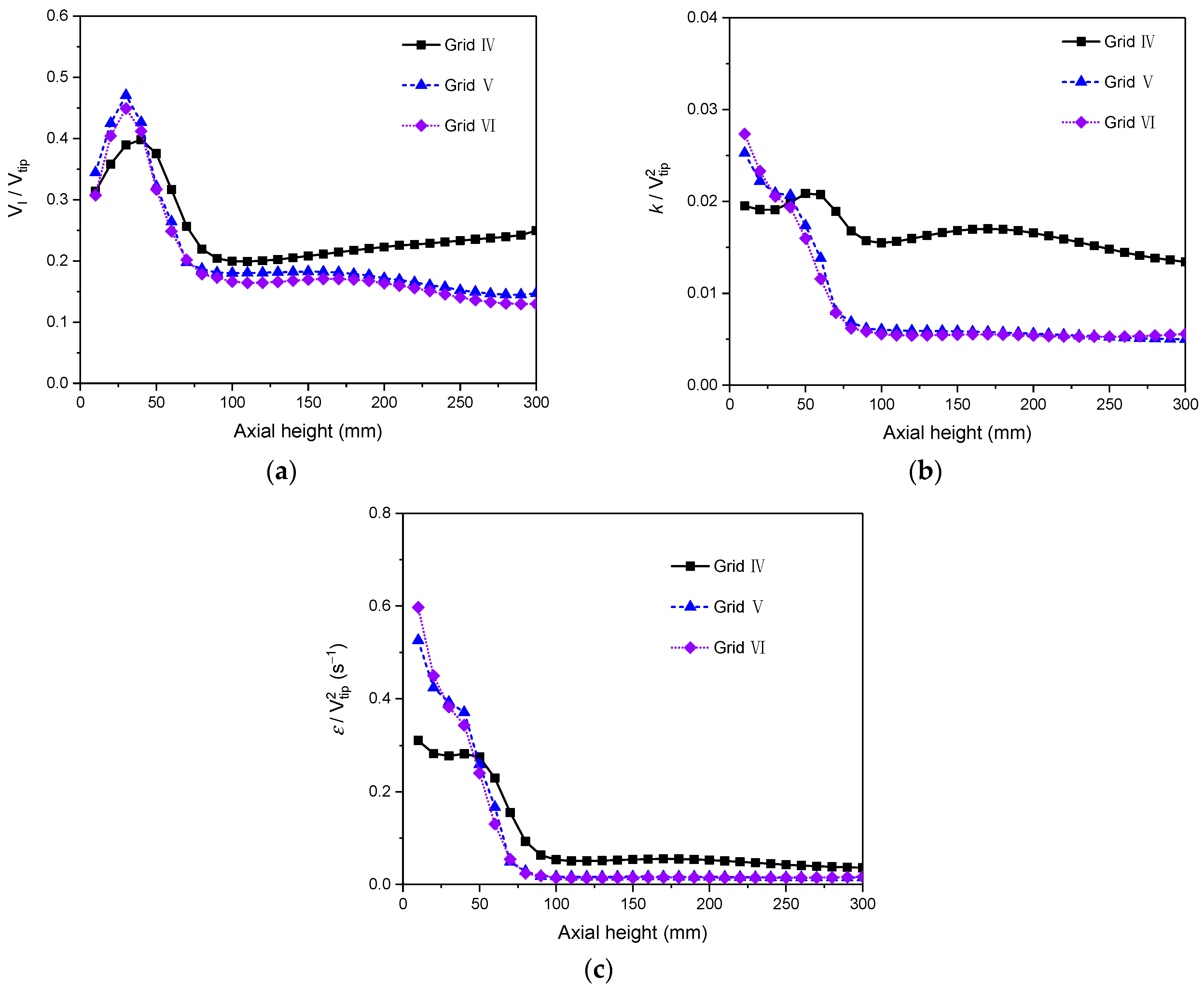
2.3.4. Grid Independency

The grid independency is tested before the simulations; see

Table 2. Influence of grid independency on simulations of Case G for BC.

Items	Grid I	Grid II	Grid III
Total number of cells	38,950	76,362	145,979
Maximum cell size (m3)	3.45 × 10−6	2.25 × 10−6	1.00 × 10−6
Minimum cell size (m3)	2.81 × 10−7	1.41 × 10−7	8.04 × 10−8

and

Table 3. Influence of grid independency on simulations of Case E for GIAT and CSTR.

Items	Grid IV	Grid V	Grid VI
Total number of cells	40,616	338,432	672,633
Maximum cell size (m3)	1.41 × 10−6	2.78 × 10−7	1.27 × 10−7
Minimum cell size (m3)	3.02 × 10−8	1.81 × 10−9	8.08 × 10−10

for the grid configurations.

Case G is used in this test for BC with three grid configurations. Hexahedral cells are generated and the grid at the inlet and liquid level is refined. The gas is mainly distributed in the center of the tank because of the inlet arrangement. Figure 4 shows the average axial distribution of liquid velocity along the tank height. The three configurations yield similar results. The mean bubble sizes predicted by PBM for the three grids from Grid I to III are 1.5, 1.6, and 1.6 mm, respectively. In addition, as reported by other researchers [60,61,62], grid refinement does not always improve the simulation accuracy in BC. Therefore, Grid II is employed for the simulations of BC.

Additionally, Case E is used in this test for GIAT and CSTR. A refined grid is generated for the regions near the impeller. The grid convergence index (GCI) [63] is used to evaluate grid independency. The methodology applied by Sosnowski [64] is adopted, and the turbulent dissipation rate over the mass [65] is selected as the objective variable. The GCI₂₁ value is 0.10% for the stirred tank. It indicates good grid convergence behavior. Furthermore, the average axial distributions of liquid velocity (V_l), turbulent kinetic energy (k), and turbulent dissipation rate (ε) at a distance of 100 mm from the reactor center are chosen for an extensive grid independency check [66]. They are normalized using the impeller tip velocity (V_tip) for ease of presentation, as shown in Figure 5. The difference between Grids IV and V is obvious, whereas the results of Grids V and VI are in reasonable agreement. It indicates that increasing the number of grids after Grid V barely improves performance. Therefore, Grid V is utilized, compromising the accuracy and computational time.

3. Results and Discussion

3.1. Effects of Agitation Speed on Degassing Efficiency

The effects of agitation speed on degassing efficiency are investigated with and without nitrogen injection. For the self-aspirated GIAT mode, the critical impeller speed for the onset of gas induction, $N_{cr}$, is 6.94 Hz. Thus, the rotational speed in GIAT ranges from 8.32 Hz to 16.70 Hz, higher than $N_{cr}$. In addition, in order to check the effect of the perforated shroud on degassing efficiency, two orifice sizes, 1.6 mm and 9.5 mm, are compared. When Q_G = 3.93 × 10⁻⁴ m³/s, the contactor functions as a CSTR with 9.5 mm shroud; the $N_{cd}$ calculated using Equation (32) is 6.14 Hz at this feeding rate.

Figure 6 shows the variation in degassing efficiency with stirring speed in both cases. In a GIAT, the degassing efficiency steadily increases with the impeller speed before reaching its plateau. Moreover, the orifice dimension of shroud insignificantly affects the degassing efficiency. This finding concurs with those reported by other researchers [16,67] who believe that $k_{L}a$ in a stirred tank is independent of the type of disperser and its orifice diameter. Specifically, the change of $k_{L}a$ is almost dependent on the change of specific interfacial area, $a$ [23]. The ultimate bubble diameter in a turbulent regime is decided by the turbulence intensity in the continuous phase imposed by energy dissipated via mechanical agitation [23,68,69]. The impact of orifice dimensions on bubble size is negligible [23]. Hence, $a$ depends on turbulence intensity; as a result, $k_{L}a$ depends on turbulence intensity [16]. Therefore, it is reasonable that the efficiency difference between the two shrouds is small.

The deviations between experiment and mathematical models when agitation speed is above 10 Hz are within ±5%. However, it is not the case when the agitation speed is 8.5 Hz, which is because the correlation used to estimate the gas induction rate does not apply to speeds approaching $N_{cr}$. The reason for this mismatch is that, at the beginning of gas induction, the gas is induced in the regions of the impeller where the fluid density reduces sharply. In addition, the pressure driving force is much lower compared to that in the absence of gas. Thus, the calculation overestimates the gas intake, resulting in an overestimation of the associated degassing efficiency [70].

No further investigation of the orifice size of a shroud is conducted in the CSTR because of its insignificant effect in GIAT. The CSTR is superior to GIAT according to degassing efficiency. However, with the increase in rotational speed, its advantage decreases. The change of degassing efficiency is not evident for the tested speeds. When the speed approaches $N_{cd}$, the degassing efficiency reaches its plateau immediately. In addition, the deviation between predictions using Equation (31) and the experiment is less than 9.3%, although the agreement is not as well as the counterpart of the GIAT.

A speed slightly above $N_{cd}$ is preferred for a CSTR because mechanical agitation contributes the most to energy consumption in the degasser and a higher speed requires a higher-quality shaft. Despite the lower efficiency of GIAT than that of a CSTR, an acceptable efficiency can be attained at a moderately greater speed. From energy and economics perspectives, a GIAT operated at a medium speed of about 10 Hz is also a suitable alternative for gas-liquid contact practice.

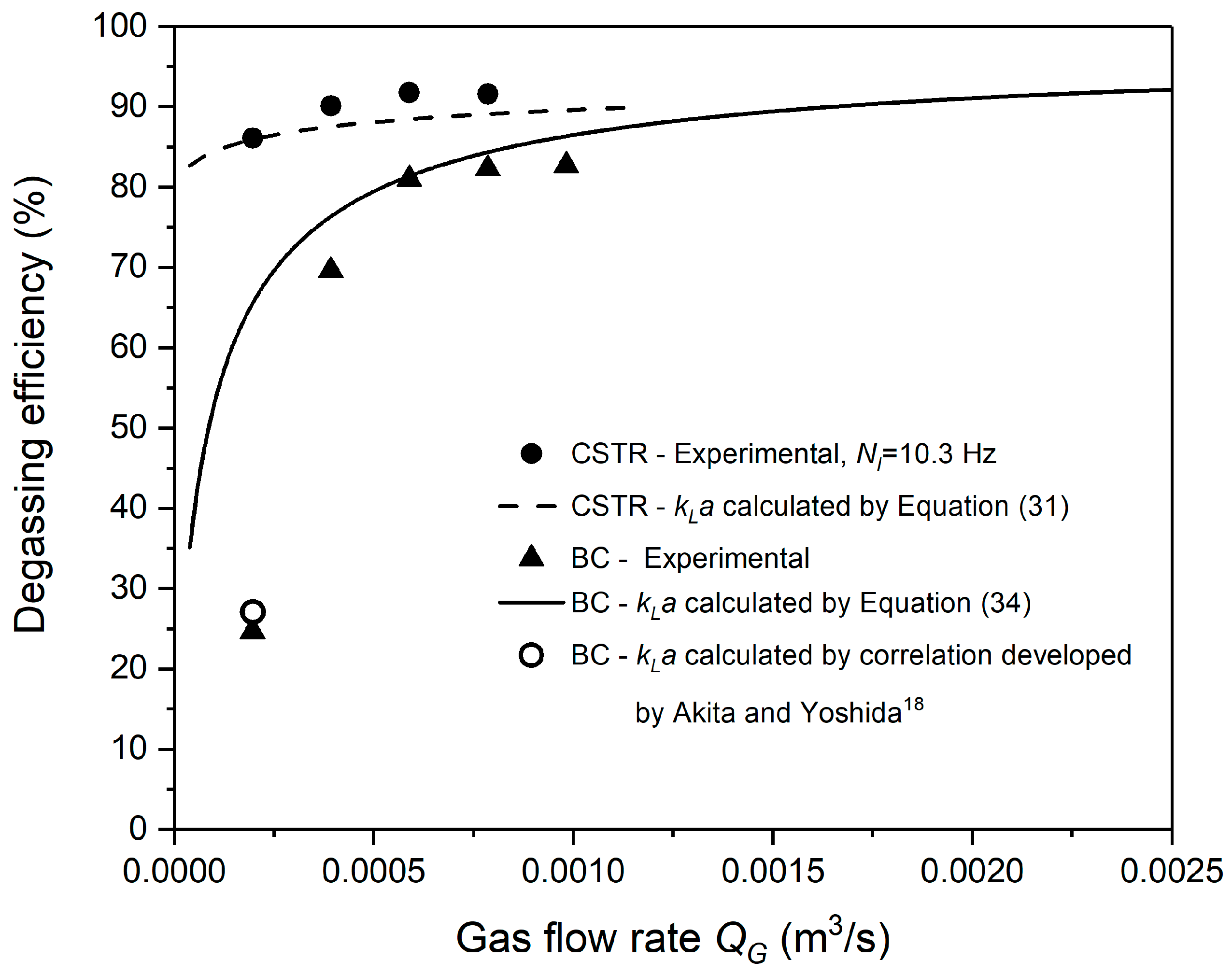
3.2. Effects of Flow Rate of Purge Nitrogen on Degassing Efficiency

Figure 7 shows the effects of various flow rates of purge nitrogen on degassing efficiencies of different reactors. For the BC with a porous media sparger, the degassing efficiency increases from 24.7% to 69.4% when the nitrogen flow rate increases from 1.97 × 10⁻⁴ to 3.93 × 10⁻⁴ m³/s, and it steadily rises to 82% or so as the plateau. Furthermore, the CSTR stirring at 10.3 Hz leads to the highest efficiencies among the investigated reactors.

The prediction of the CSTR using Equation (31) is in good agreement with the experimental data, as indicated by the discrepancy within ±3.3%. The degassing performance of BC is strongly associated with the type of sparger, which is different from CSTR. The porous media sparger is well-known for efficient gas distribution, whose $k_{L}a$ is usually evaluated by Equation (34). The corresponding model can then predict most efficiencies within ±9.1% of experimental data except for the first data point of BC at Q_G = 1.97 × 10⁻⁴ m³/s. This mismatch probably arises because the first data point is collected at Q_G = 1.97 × 10⁻⁴ m³/s, under which U_G = 0.0012 m/s. It is not within the applicable range of superficial gas velocity (0.0025–0.08 m/s) in Equation (34). However, there is a deviation of 9.7% between the experimental data of this data point and prediction based on the $k_{L}a$ correlation for inferior gas distributors reported by Akita and Yoshida [18]. It means that the gas cannot be effectively distributed at this gas flow rate because of the uneven use of porous media.

Overall, the degassing performance of CSTR is the best in this paper. The increase in efficiency is less than 1%, when the gas flow rate is beyond 3.93 × 10⁻⁴ m³/s, around which can be set as the optimum rate. Furthermore, the mathematical model shows that the degassing efficiency of the BC can be more than 86%, when the gas flow rate is higher than 9.48 × 10⁻⁴ m³/s. This indicates that at relatively higher gas flow rates, the degassing efficiency of BC is comparable to that of CSTR. Considering advantages such as no movement part, less maintenance and footprint, efficient BCs performed at gas flow rates around 7.87 × 10⁻⁴ m³/s are also potential candidates for gas-liquid contact.

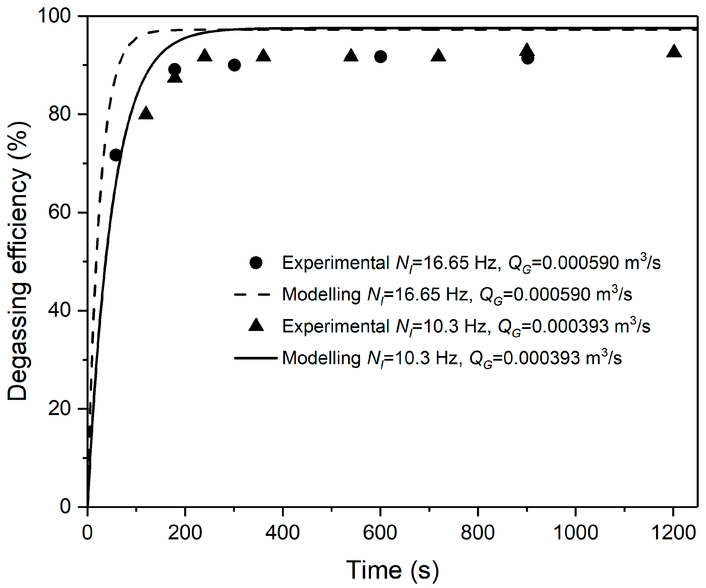
3.3. Degassing Efficiencies of a Semi-Batch Reactor

First, we identify the contribution of the horizontal pipe to the overall continuous degassing efficiency, ${\eta }_{con}$. Equation (24) in Section 2.2.1 indicates that the contribution of the pipe to ${\eta }_{con}$ is 2.46% for Z = 419.1 mm, Q_G = 3.93 × 10⁻⁴ m³/s, and Q_L = 1.26 × 10⁻⁴ m³/s. Under this condition, the overall degassing efficiency calculated using Equations (25), (33) and (34) is 76.34% for a BC and that calculated using Equations (25), (31) and (33) is 87.55% for a CSTR at $N_I$ = 10.3 Hz. These results show that the contribution of pipe to ${\eta }_{con}$ is negligible for both reactors. Therefore, in the semi-batch model, the pipe part can be ignored for simplicity with insignificant error.

Figure 8 shows the change of degassing efficiency varying with residence time in the semi-batch contactor, which is operated batch-wise and continuous modes concerning liquid and gas phases, respectively. The mathematical model is validated under the two conditions: the differences between the model and experiments are within 9.1% at $N_I$ = 10.3 Hz and Q_G = 0.000393 m³/s; they are within 8.4% with the exception of the first data point at $N_I$ = 16.65 Hz and Q_G = 0.00059 m³/s.

The capacity of a degassing device is important to engineering practice. The degassing capacity is defined by the upper limit of degassing efficiency. According to Equation (38), it is tied to the inlet gas composition and initial DO concentration. The initial DO concentration is ten ppm in this work. The theoretical capacity can reach 97.6% for nitrogen of industrial grade (i.e., 99.5% purity). Figure 8 shows an experimental capacity of 92%. The deviation between theoretical and experimental degassing capacity is 6.1%, which is acceptable in engineering modelling. The change in physicochemical properties of the gas phase during the bubble motion may further optimize the prediction.

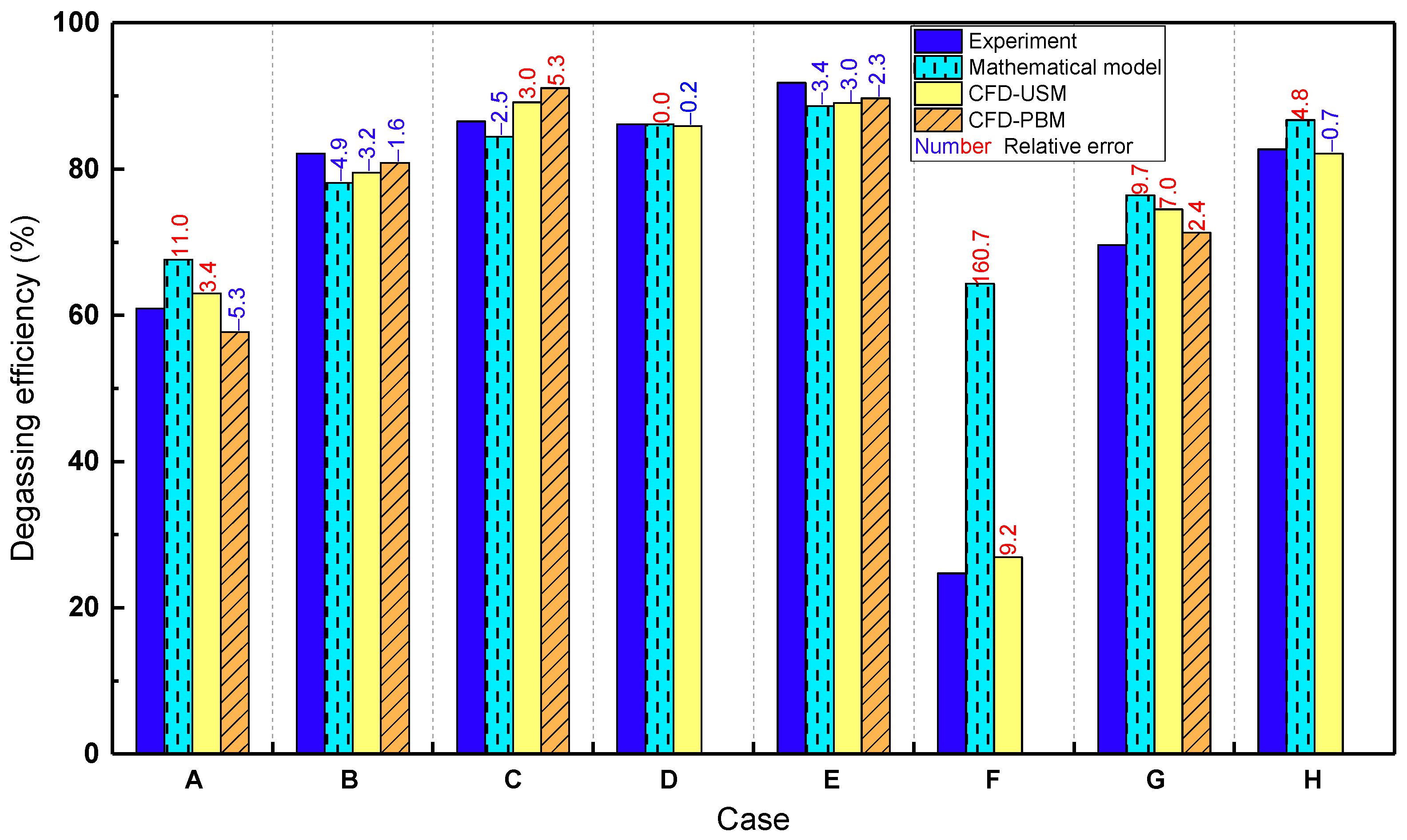
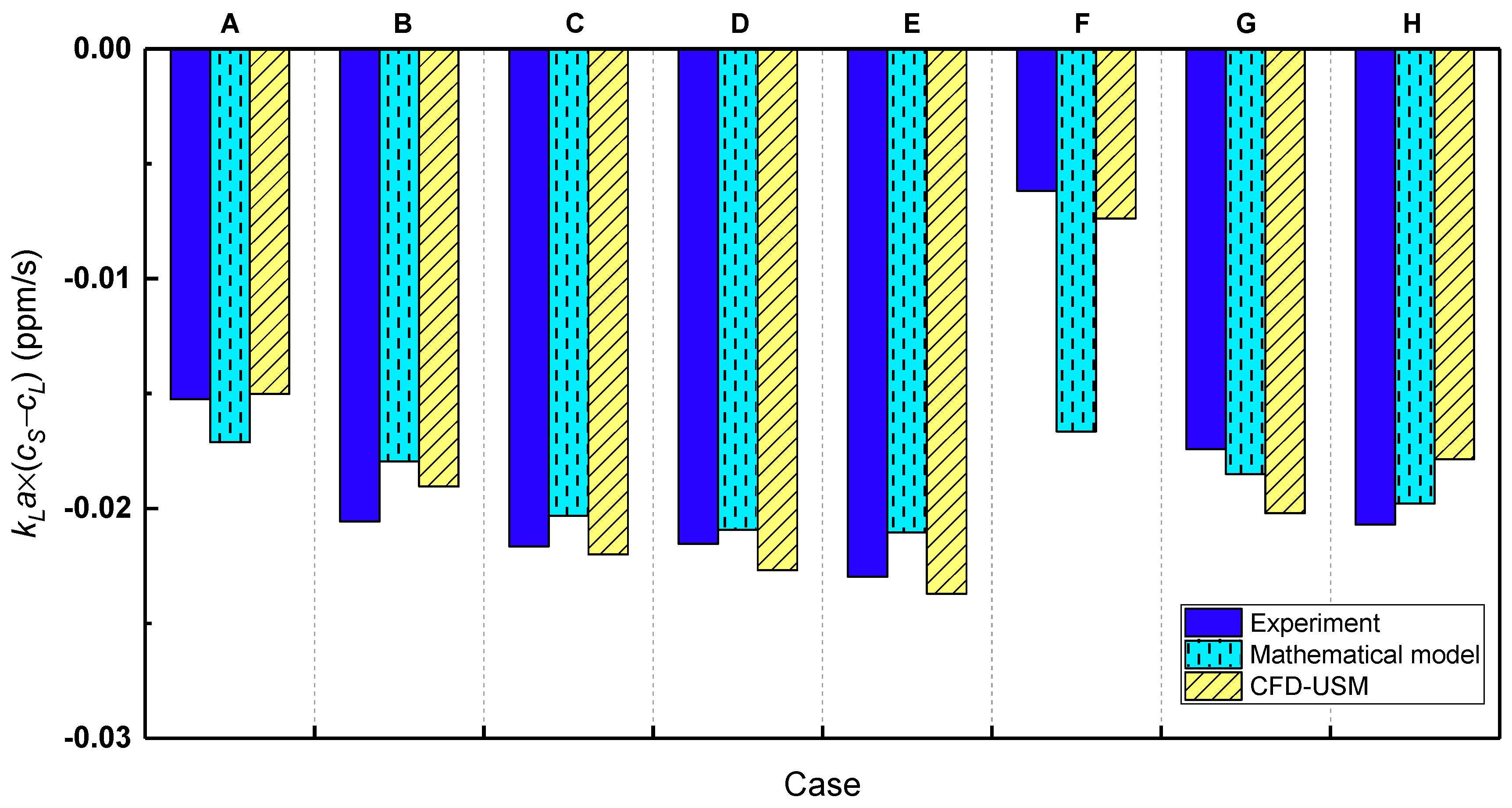
3.4. Comparison between Mathematical and CFD Models

Figure 9 compares the mathematical models with CFD models for eight representative cases. In the CFD simulations, the relative errors between experiments and CFD predicted values are all within ±10% and are generally less than those of mathematical models.

Cases A and F, in which the mathematical models behave poorly (relative errors exceed 10%, even more than 160% in Case F), deserve special investigation. Case A describes the first data point of the GIAT at N_I = 8.3 Hz in Figure 6. The CFD models predict more accurately than the mathematical model does. The CFD coupled with USM slightly overestimates the degassing efficiency, whereas the CFD coupled with PBM underestimates that. However, the gas induction rate is also calculated by Equation (27) in CFD modelling; hence, modelling the self-induction process driven by negative pressure in future work can further evaluate the degassing performance of a GIAT. Case F represents the first data point of the BC (Q_G = 1.97 × 10⁻⁴ m³/s) in Figure 7; a simulation with 5 mm uniform bubble size results in a relative error of 9.2%, which is much better than the relative error of 160.7% produced by the mathematical model.

Table 4. Comparison of bubble sizes used in CFD-USM and predicted by CFD-PBM models.

Case No.	Reactor	Uniform Bubble Size Used in CFD-USM (mm)	Mean Bubble Size Predicted by CFD-PBM (mm)
A	GIAT *	3.5	3.4
B	GIAT	4.0	4.1
C	GIAT	5.0	4.4
E	CSTR	2.5	2.1
G	BC	1.5	1.6

* GIAT means GIAT with a 9.5-mm shroud.

presents the comparison between the uniform bubble sizes used in CFD-USM and the mean sizes predicted by CFD-PBM models. In GIAT (i.e., Cases A, B, and C), larger uniform bubble size is adopted for higher agitation speed. The mean bubble sizes predicted by CFD-PBM show the same trend. Additionally, the CFD-PBM model with the same settings is suitable for the reactor under a wide range of operating conditions. Although different factors of coalescence and breakage kernels in PBM model are adopted, the same inlet bubble size is appropriate for both the CSTR and BC (i.e., Cases E and G), as shown in Table 1. Additionally, the contours of Sauter mean diameter along with local bubble size distribution at several positions in three cases are presented in Figure 10. In the GIAT and CSTR, smaller bubbles distribute near the impeller and jet stream because of relatively high turbulent dissipation rate [71].

Figure 11 compares experimental global $k_{L}a\times \left(c_s-c_L\right)$ values [15] with those predicted by mathematical and CFD-USM models. The approximation of $c_L=c_{Lout}$ is adopted in the mathematical model. Conversely, the volume average $k_{L}a\times \left(c_s-c_L\right)$ is calculated in the CFD model. Overall, CFD slightly outperforms its mathematical counterpart. This justifies the rational of assumptions in the mathematical models, such as a perfect mixing of gas-liquid contact. As shown in Figure 12, when the degassing systems reach dynamic equilibrium, the distribution of DO is visibly homogeneous except for the region near the inlet.

Besides, the contours of $k_{L}a$, $k_L$, and $a$ in each case using CFD-USM simulation are shown in Figures S1–S3. The $k_{L}a$ values calculated by mathematical models, i.e., $k_L{a}^{*}$, are highlighted in the labeled color bars for comparison. For $k_{L}a$, the predicted values of mathematical models fall within the ranges of CFD results. Overall, the variation in $k_L$ values predicted by the two mass transfer models is small in these reactors. The $k_{L}a$ value almost depends on $a$, which is consistent with previous findings [19]. For GIAT (see Figure S1), with the increase in agitation speed, $a$ increases as the gas induction rate increases. For CSTR (see Figure S2), the increasing gas flow rate also mainly leads to larger $a$. For BC (see Figure S3), compared to Case F, not only $a$, but also $k_L$ in Cases G and H is significantly increased. The effective gas-liquid mass transfer is achieved in GIAT and CSTR by impeller rotation [66]. The $k_L$ in these two degassers is predicted by the turbulent dissipation rate. Thus, $k_L$ is visibly bigger near the blades with higher turbulent dissipation rates (see Figure 13). However, in BC with porous media sparger, the location of gas inlet results in gas concentrating in the center of the tank (see Figure S3).

Furthermore, the mathematical models predict the variations of degassing efficiency with acceptable accuracy at a low cost. They are maybe preferred in practice because of the compromise between computational cost and accuracy. However, the mathematical models are restricted to specific operating conditions and reactor configurations due to the use of empirical correlations. Conversely, CFD models provide more accurate results at high computational cost. They can also reveal more local details inside reactors. For instance, the mathematical models cannot well interpret the low efficiency at relatively low gas flow rate for BC with porous media sparger in Case F; CFD results clearly show the relatively low values of $a$ and $k_L$, resulting in inefficient mass transfer. The combination of these two kinds of models helps to understand the degassing system better, and guides its modification and optimization. Moreover, coupling CFD with optimization algorithms (e.g., multiobjective evolutionary algorithm [72]) to efficiently optimize reactor configuration for maximizing degassing efficiency can be explored in the future.

4. Conclusions

In the mathematical models, the mass transfer coefficients vary from reactor to reactor. The continuous reactor model based on complete mixing assumption can interpret the impacts of different parameters on degassing efficiency within ±13% for all three types of reactors except for the first data points of the GIAT at $N_I$ = 8.3 Hz and the BC at Q_G = 1.97 × 10⁻⁴ m³/s. The semi-batch model evaluates the degasser performance with relative errors within 9.1% at Q_G = 0.000393 m³/s and $N_I$ = 10.3 Hz, as well as within 8.4% except for the first data point at Q_G = 0.00059 m³/s and $N_I$ = 16.65 Hz. The empirical correlations to estimate the overall $k_{L}a$ values have been proven applicable in these three reactors. Compared to mathematical models, CFD models are generally superior. Moreover, CFD-PBM can perform better. The relative errors are all within ±10%.

The mathematical models benefit the selection of efficient degassing contactors and determination of optimum operation parameters. The CSTR affords better performance than the GIAT and BC do. A speed slightly above $N_{cd}$ and a gas flow rate around 3.93 × 10⁻⁴ m³/s are desired for a CSTR in practice. A GIAT operated at a medium speed of about 10 Hz is also a suitable alternative for gas-liquid contactor. Furthermore, a BC equipped with porous media sparger at a gas flow rate around 7.87 × 10⁻⁴ m³/s is a potential candidate of degassing technology. It is noted that the accuracy of mathematical models depends heavily on specific empirical formulas.

In comparison, although the CFD model has a high computational cost, it can reveal the flow and reaction characteristics and directly provide the contours of $k_{L}a$, $k_L$, and $a$ inside reactors in a broader range of operating conditions. This makes CFD simulation appropriate for harsh industrial scenarios such as the removal of hydrogen sulfide from liquid sulfur in which the empirical correlations for important quantities are unavailable. Thus, the CFD model is useful for reactor optimization, such as impeller configurations, which is the subject of future study.

References

1. Lei, H. Experimental and Modeling Studies of Bubble Degassing. Master’s Thesis, University of Calgary, Calgary, AB, Canada, 2010. [Google Scholar]
2. Yu, D. Simulation Studies on Water Deoxygenation Process in A Rotating Packed Bed. Master’s Thesis, Dalian University of Technology, Dalian, China, 2014. [Google Scholar]
3. Zhao, Z.; Liu, Z.; Xiang, Y.; Arowo, M.; Shao, L. Removal of Dissolved Oxygen from Water by Nitrogen Stripping Coupled with Vacuum Degassing in a Rotor-Stator Reactor. Processes 2021, 9, 1354. [Google Scholar] [CrossRef]
4. Yu, S. Numerical Modeling of Dehydrogenation and Denitrogenation in Industrial Vacuum Tank Degassers. Ph.D. Thesis, Aalto University, Helsinki, Finland, 2014. [Google Scholar]
5. Riedel, E.; Köhler, P.; Ahmed, M.; Hellmann, B.; Horn, I.; Scharf, S. Industrial suitable and digitally recordable application of ultrasound for the enviromentally friendly degassing of aluminium melts before tilt casting. Procedia CIRP 2021, 98, 589–594. [Google Scholar] [CrossRef]
6. Xie, D.; Wu, P.; Wu, D. The Design of a Degassing Pump Based on Numerical and Experimental Research. In Proceedings of the ASME/JSME/KSME 2015 Joint Fluids Engineering Division Summer Meeting, Seoul, Republic of Korea, 26–31 July 2015. [Google Scholar]
7. Che, D.; Yao, g.; Kang, W.; Zhang, X. Effect of Vacuum Degassing on Composites preparation. In Proceedings of the TMS 2010 Annual Meeting Supplemental Proceedings on Materials Processing and Properties, Seattle, WA, USA, 14–18 February 2010; pp. 301–306. [Google Scholar]
8. Oosterom, S.v.; Schreier, A.; Battley, M.; Bickerton, S.; Allen, T. Influence of dissolved gasses in epoxy resin on resin infusion part quality. Compos. Part A Appl. Sci. Manuf. 2020, 132, 105818. [Google Scholar] [CrossRef]
9. Juan, J.; Silva, A.; Tornero, J.A.; Gámez, J.; Salán, N. Void Content Minimization in Vacuum Infusion (VI) via Effective Degassing. Polymers 2021, 13, 2876. [Google Scholar] [CrossRef] [PubMed]
10. Yu, H.; The, J.; Tan, Z.; Feng, X. Modeling SO2 absorption into water accompanied with reversible reaction in a hollow fiber membrane contactor. Chem. Eng. Sci. 2016, 156, 136–146. [Google Scholar] [CrossRef]
11. Astarita, G. Mass transfer with chemical reaction. Ind. Eng. Chem. 1967, 58, 379–383. [Google Scholar]
12. Ma, Q.; Shang, C.; Zhang, G.; Fang, H. Numerical Investigation of Degassing Behavior of Highly Viscous Non-Newtonian Fluids under Stirring. Chem. Eng. Technol. 2020, 43, 157–167. [Google Scholar] [CrossRef]
13. Jaszczur, M.; Mlynarczykowska, A. A General Review of the Current Development of Mechanically Agitated Vessels. Processes 2020, 8, 982. [Google Scholar] [CrossRef]
14. Tari, F.; Zarrinpashne, S.; Shekarriz, M.; Ruzbehani, A. Modeling of mass transfer and hydrodynamic investigation of H2S removal from molten sulfur using porous Sparger. Heat Mass Transf. 2020, 56, 1641–1648. [Google Scholar] [CrossRef]
15. Yu, H.S.; Tan, Z.C. New Correlations of Volumetric Liquid-Phase Mass Transfer Coefficients in Gas-Inducing Agitated Tank Reactors. Int. J. Chem. React. Eng. 2012, 10, 1585–1611. [Google Scholar] [CrossRef]
16. Yawalkar, A.A.; Heesink, A.B.M.; Versteeg, G.F.; Pangarkar, V.G. Gas-liquid mass transfer coefficient in stirred tank reactors. Can. J. Chem. Eng. 2002, 80, 840–848. [Google Scholar] [CrossRef] [Green Version]
17. Kapic, A.; Heindel, T.J. Correlating gas-liquid mass transfer in a stirred-tank reactor. Chem. Eng. Res. Des. 2006, 84, 239–245. [Google Scholar] [CrossRef]
18. Akita, K.; Yoshida, F. Gas Holdup and Volumetric Mass Transfer Coefficient in Bubble Columns. Effects of Liquid Properties. Ind. Eng. Chem. Process Des. Dev. 1973, 12, 76–80. [Google Scholar] [CrossRef]
19. Manjrekar, O.N. Hydrodynamics and Mass Transfer in Bubble Columns. Ph.D. Thesis, Washington University, St. Louis, MO, USA, 2016. [Google Scholar]
20. Deckwer, W.D.; Burckhart, R.; Zoll, G. Mixing and mass transfer in tall bubble columns. Chem. Eng. Sci. 1974, 29, 2177–2188. [Google Scholar] [CrossRef]
21. Guo, K.Y.; Wang, T.F.; Liu, Y.F.; Wang, J.F. CFD-PBM simulations of a bubble column with different liquid properties. Chem. Eng. J. 2017, 329, 116–127. [Google Scholar] [CrossRef]
22. Zhang, H.H.; Sayyar, A.; Wang, Y.L.; Wang, T.F. Generality of the CFD-PBM coupled model for bubble column simulation. Chem. Eng. Sci. 2020, 219, 115514. [Google Scholar] [CrossRef]
23. Sideman, S.; Hortasu, N.; Fulton, J.W. Mass transfer in gas-liquid contacting systems. Ind. Eng. Chem. 2002, 58, 32–47. [Google Scholar] [CrossRef]
24. Ramkrishna, D. Population Balances Theory and Applications to Particulate Systems in Engineering; Academic Press: San Diego, CA, USA, 2000. [Google Scholar]
25. Li, L.; Hao, R.; Jin, X.; Hao, Y.; Fu, C.; Zhang, C.; Gu, X. A Turbulent Mass Diffusivity Model for Predicting Species Concentration Distribution in the Biodegradation of Phenol Wastewater in an Airlift Reactor. Processes 2023, 11, 484. [Google Scholar] [CrossRef]
26. Higbie, R. The rate of absorption of a pure gas into a still liquid during short periods of exposure. Trans. AIChE 1935, 31, 365–377. [Google Scholar]
27. Lamont, J.C.; Scott, D.S. An eddy cell model of mass transfer into the surface of a turbulent liquid. AIChE J. 1970, 16, 513–519. [Google Scholar] [CrossRef]
28. Wang, T.F.; Wang, J.F. Numerical simulations of gas-liquid mass transfer in bubble columns with a CFD-PBM coupled model. Chem. Eng. Sci. 2007, 62, 7107–7118. [Google Scholar] [CrossRef]
29. Buffo, A.; Vanni, M.; Marchisio, D.L. Multidimensional population balance model for the simulation of turbulent gas-liquid systems in stirred tank reactors. Chem. Eng. Sci. 2012, 70, 31–44. [Google Scholar] [CrossRef]
30. Petitti, M.; Vanni, M.; Marchisio, D.L.; Buffo, A.; Podenzani, F. Simulation of coalescence, break-up and mass transfer in a gas-liquid stirred tank with CQMOM. Chem. Eng. J. 2013, 228, 1182–1194. [Google Scholar] [CrossRef]
31. Moreno-Casas, P.A.; Scott, F.; Delpiano, J.; Abell, J.A.; Caicedo, F.; Munoz, R.; Vergara-Fernandez, A. Mechanistic Description of Convective Gas-Liquid Mass Transfer in Biotrickling Filters Using CFD Modeling. Environ. Sci. Technol. 2020, 54, 419–426. [Google Scholar] [CrossRef] [PubMed]
32. Enersul. CUSTOM SULPHUR DEGASSING-HYSPEC™ Degassing Systems. Available online: https://www.enersul.com/degassing (accessed on 30 May 2023).
33. Yu, H. Absorption of Nitric Oxide from Flue Gas Using Ammoniacal Cobalt(II) Solutions. Ph.D. Thesis, University of Waterloo, Waterloo, ON, Canada, 2012. [Google Scholar]
34. Mandhane, J.M.; Gregory, G.A.; Aziz, K. A flow pattern map for gas-liquid flow in horizontal pipes. Int. J. Multiph. Flow 1974, 1, 537–553. [Google Scholar] [CrossRef]
35. Jepsen, J.C. Mass transfer in two-phase flow in horizontal pipelines. AIChE J. 1970, 16, 705–711. [Google Scholar] [CrossRef]
36. Taitel, Y.; Dukler, A.E. A theoretical approach to the Lockhart-Martinelli correlation for stratified flow. Int. J. Multiph. Flow 1976, 2, 591–595. [Google Scholar] [CrossRef]
37. Chen, J.J.J.; Spedding, P.L. An analysis of holdup in horizontal two-phase gas-liquid flow. Int. J. Multiph. Flow 1983, 9, 147–159. [Google Scholar] [CrossRef]
38. Spedding, P.L.; Hand, N.P. Prediction in stratified gas-liquid co-current flow in horizontal pipelines. Int. J. Heat Mass Transf. 1997, 40, 1923–1935. [Google Scholar] [CrossRef]
39. Forrester, S.E.; Rielly, C.D.; Carpenter, K.J. Gas-inducing impeller design and performance characteristics. Chem. Eng. Sci. 1998, 53, 603–615. [Google Scholar] [CrossRef]
40. Akita, K.; Yoshida, F. Bubble Size, Interfacial Area, and Liquid-Phase Mass Transfer Coefficient in Bubble Columns. Ind. Eng. Chem. Process Des. Dev. 1974, 13, 84–91. [Google Scholar] [CrossRef]
41. Kresta, S.M.; Mao, D.M.; Roussinova, V. Batch blend time in square stirred tanks. Chem. Eng. Sci. 2006, 61, 2823–2825. [Google Scholar] [CrossRef]
42. Deckwer, W.D.; Nguyen-Tien, K.; Kelkar, B.G.; Shah, Y.T. Applicability of axial dispersion model to analyze mass transfer measurements in bubble columns. AIChE J. 1983, 29, 915–922. [Google Scholar] [CrossRef]
43. Yu, H.S.; Tan, Z.C. On the Kinetics of the Absorption of Nitric Oxide into Ammoniacal Cobalt(II) Solutions. Environ. Sci. Technol. 2014, 48, 2453–2463. [Google Scholar] [CrossRef]
44. Yu, H.S.; Tan, Z.C.; The, J.; Feng, X.S.; Croiset, E.; Anderson, W.A. Kinetics of the Absorption of Carbon Dioxide into Aqueous Ammonia Solutions. AIChE J. 2016, 62, 3673–3684. [Google Scholar] [CrossRef]
45. Linek, V.; Vacek, V.; Bene, P. A critical review and experimental verification of the correct use of the dynamic method for the determination of oxygen transfer in aerated agitated vessels to water, electrolyte solutions and viscous liquids. Chem. Eng. J. 1987, 34, 11–34. [Google Scholar] [CrossRef]
46. Robinson, C.W.; Wilke, C.R. Oxygen absorption in stirred tanks: A correlation for ionic strength effects. Biotechnol. Bioeng. 1973, 15, 755–782. [Google Scholar] [CrossRef]
47. ANSYS Inc. ANSYS Fluent Theory Guide; ANSYS Inc.: Canonsburg, PA, USA, 2020. [Google Scholar]
48. Sato, Y.; Sekoguchi, K. Liquid velocity distribution in two-phase bubble flow. Int. J. Multiph. Flow 1975, 2, 79–95. [Google Scholar] [CrossRef]
49. Seidel, S.; Eibl, D. Influence of Interfacial Force Models and Population Balance Models on the k(L)a Value in Stirred Bioreactors. Processes 2021, 9, 1185. [Google Scholar] [CrossRef]
50. Wang, M.; Ni, C.; Bu, X.; Peng, Y.; Xie, G.; Tan, Z.; Yu, H. CFD-PBM Simulation of the Column Flotation Unit of FCMC: Importance of Gas-Liquid Interphase Forces Models. Can. J. Chem. Eng. 2023, 1, 1–16. [Google Scholar] [CrossRef]
51. ANSYS Inc. ANSYS Fluent User’s Guide; ANSYS Inc.: Canonsburg, PA, USA, 2020. [Google Scholar]
52. Prince, M.J.; Blanch, H.W. Bubble coalescence and break-up in air-sparged bubble columns. AIChE J. 1990, 36, 1485–1499. [Google Scholar] [CrossRef]
53. Luo, H.; Svendsen, H.F. Theoretical model for drop and bubble breakup in turbulent dispersions. AIChE J. 2010, 42, 1225–1233. [Google Scholar] [CrossRef]
54. Maluta, F.; Paglianti, A.; Montante, G. A PBM-Based Procedure for the CFD Simulation of Gas-Liquid Mixing with Compact Inline Static Mixers in Pipelines. Processes 2023, 11, 198. [Google Scholar] [CrossRef]
55. Liu, M. Age distribution and the degree of mixing in continuous flow stirred tank reactors. Chem. Eng. Sci. 2012, 69, 382–393. [Google Scholar] [CrossRef]
56. Lane, G.L. Improving the accuracy of CFD predictions of turbulence in a tank stirred by a hydrofoil impeller. Chem. Eng. Sci. 2017, 169, 188–211. [Google Scholar] [CrossRef]
57. Aubin, J.; Fletcher, D.; Xuereb, C. Modeling turbulent flow in stirred tanks with CFD: The influence of the modeling approach, turbulence model and numerical scheme. Exp. Therm. Fluid Sci. 2004, 28, 431–445. [Google Scholar] [CrossRef] [Green Version]
58. Wu, M.; Jurtz, N.; Walle, A.; Kraume, M. Evaluation and application of efficient CFD-based methods for the multi-objective optimization of stirred tanks. Chem. Eng. Sci. 2022, 263, 118109. [Google Scholar] [CrossRef]
59. Guan, X.; Li, X.; Yang, N.; Liu, M. CFD simulation of gas-liquid flow in stirred tanks: Effect of drag models. Chem. Eng. J. 2020, 386, 121554. [Google Scholar] [CrossRef]
60. Law, D.; Battaglia, F.; Heindel, T.J. Model validation for low and high superficial gas velocity bubble column flows. Chem. Eng. Sci. 2008, 63, 4605–4616. [Google Scholar] [CrossRef]
61. Monahan, S.M.; Vitankar, V.S.; Fox, R.O. CFD predictions for flow-regime transitions in bubble columns. AIChE J. 2005, 51, 1897–1923. [Google Scholar] [CrossRef]
62. Picardi, R.; Zhao, L.; Battaglia, F. On the Ideal Grid Resolution for Two-Dimensional Eulerian Modeling of Gas–Liquid Flows. J. Fluids Eng. 2016, 138, 114503. [Google Scholar] [CrossRef]
63. Roache, P.J. Perspective: A Method for Uniform Reporting of Grid Refinement Studies. J. Fluids Eng. 1994, 116, 405–413. [Google Scholar] [CrossRef]
64. Sosnowski, M. Evaluation of Heat Transfer Performance of a Multi-Disc Sorption Bed Dedicated for Adsorption Cooling Technology. Energies 2019, 12, 4660. [Google Scholar] [CrossRef] [Green Version]
65. Maluta, F.; Buffo, A.; Marchisio, D.L.; Montante, G.; Paglianti, A.; Vanni, M. Effect of turbulent kinetic energy dissipation rate on the prediction of droplet size distribution in stirred tanks. Int. J. Multiph. Flow 2021, 136, 103547. [Google Scholar] [CrossRef]
66. Li, D.; Chen, W. Effects of impeller types on gas-liquid mixing and oxygen mass transfer in aerated stirred reactors. Process Saf. Environ. Prot. 2022, 158, 360–373. [Google Scholar] [CrossRef]
67. Garcia-Ochoa, F.; Castro, E.G. Estimation of oxygen mass transfer coefficient in stirred tank reactors using artificial neural networks. Enzym. Microb. Tech. 2001, 28, 560–569. [Google Scholar] [CrossRef]
68. Miller, D.N. Scale-up of agitated vessels gas-liquid mass transfer. AIChE J. 1974, 20, 445–453. [Google Scholar] [CrossRef]
69. Calderbank, P.H. Physical rate process in industrial fermentation. Part II. Mass transfer coefficients in gas–liquid contacting with and without mechanical agitation. Trans. Inst. Chem. Eng. 1959, 37, 173–185. [Google Scholar]
70. Sawant, S.B.; Joshi, J.B.; Pangarkar, V.G.; Mhaskar, R.D. Mass transfer and hydrodynamic characteristics of the Denver type of flotation cells. Chem. Eng. J. 1981, 21, 11–19. [Google Scholar] [CrossRef]
71. Basavarajappa, M.; Miskovic, S. Investigation of gas dispersion characteristics in stirred tank and flotation cell using a corrected CFD-PBM quadrature-based moment method approach. Miner. Eng. 2016, 95, 161–184. [Google Scholar] [CrossRef]
72. Chen, M.N.; Wang, J.J.; Zhao, S.W.; Xu, C.Z.; Feng, L.F. Optimization of Dual-Impeller Configurations in a Gas-Liquid Stirred Tank Based on Computational Fluid Dynamics and Multiobjective Evolutionary Algorithm. Ind. Eng. Chem. Res. 2016, 55, 9054–9063. [Google Scholar] [CrossRef]
73. Ranganathan, P.; Sivaraman, S. Investigations on hydrodynamics and mass transfer in gasliquid stirred reactor using computational fluid dynamics. Chem. Eng. Sci. 2011, 66, 3108–3124. [Google Scholar] [CrossRef]
Figure 1. Schematic of the lab-scale liquid degassing system.
Processes 11 01780 g001
Figure 2. (a) Cross section and (b) an infinitesimal element of an ideal horizontal gas-liquid stratified flow.
Processes 11 01780 g002
Figure 3. Computational domains and grids of (a) BC-76,362 cells and (b) GIAT and CSTR-338,432 cells.
Processes 11 01780 g003
Figure 4. The average axial distribution of liquid velocity in Case G.
Processes 11 01780 g004
Figure 5. The average axial distribution of (a) liquid velocity, (b) turbulent kinetic energy, and (c) turbulent dissipation rate in Case E at a distance of 100 mm from the reactor center.
Processes 11 01780 g005
Figure 6. Effects of agitation speed on degassing efficiency in GIAT and CSTR.
Processes 11 01780 g006
Figure 7. Effects of flow rate of nitrogen on degassing efficiency for CSTR and BC.
Processes 11 01780 g007
Figure 8. Degassing efficiency of the semi-batch degasser under different conditions.
Processes 11 01780 g008
Figure 9. Comparison of degassing efficiencies predicted by mathematical and CFD models.
Processes 11 01780 g009
Figure 10. The contours of Sauter mean diameter and local bubble size distribution calculated by PBM in (a) Case B, (b) Case E, and (c) Case G.
Processes 11 01780 g010
Figure 11. Comparison of global k L a × ( c s c L ) predicted by mathematical and CFD-USM models.
Processes 11 01780 g011
Figure 12. Contours of dissolved oxygen in liquid phase in (a) Case E for CSTR and (b) Case H for BC using CFD-USM (as examples).
Processes 11 01780 g012
Figure 13. Contours of (a) turbulent dissipation rate, (b) k L , and (c) k L a in Case E using CFD-USM for CSTR (as an example).
Processes 11 01780 g013